The number of inscribed and circumscribed
graphs of a convex polyhedron
Abstract.
In the paper we prove that the number of graphs inscribed into graph of a convex polyhedron and circumscribed around another graph does not exceed 4. For this we first studied Poncelet type problem about the number of convex -gons inscribed into one convex -gon and circumscribed around another convex -gon. It is proved that their number is also at most 4. This contrasts with Poncelet type porisms where usually infinitude of such polygons is proved, provided that one such polygon already exists. An inequality involving ratio of lengths of line segments is used. Alternative way of using Maclaurin-Braikenridge’s conic generation method is also discussed. Properties related to constructibility with straightedge and compass are also studied. A new proof, based on mathematical induction, of generalized Maclaurin- Braikenridge’s theorem is given. We also gave examples of regular polygons and a polyhedron for which number 4 is realized.
Key words and phrases:
Octahedron, graph, inscribed graph, polyhedron, porism, Poncelet type theorems, inscribed polygon, circumscribed polygon, Maclaurin’s conic generation, Braikenridge’s theorem, geometric inequality, polytopes.1991 Mathematics Subject Classification:
Primary 52B05, 51M20, 51M04; Secondary 51M15, 51M16, 52B10, 52B11, 52C051. Introduction
Polyhedra can be defined in various generality as geometric objects consisted of vertices (points), edges (line segments), and faces (polygons). Regular (Platonic), semi-regular (Archimedean), regular star polyhedra (Kepler–Poinsot), and other types of polyhedra frequently appear in mathematics, biology, crystallography, physics, etc. Convex polyhedra which are defined as convex hull of finitely many points in space play important role in geometry and its applications. Some of these polyhedra are obtained by choosing its vertices on the edges of another polyhedron and this process can be repeated indefinitely. For example, midpoints of the edges of tetrahedron give the vertices of an octahedron, whose edge midpoints give the vertices of an icosahedron. The midpoints of icosahedron and dodecahedron both give the vertices of icosidodecahedrons. The literature about history, classification, and applications of these polyhedra is extensive (see [13] and its references). In the current paper a general result is proved about the graphs of such nested polyhedra.
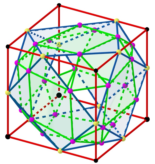
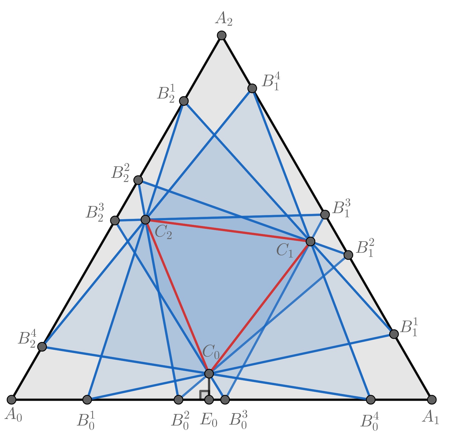
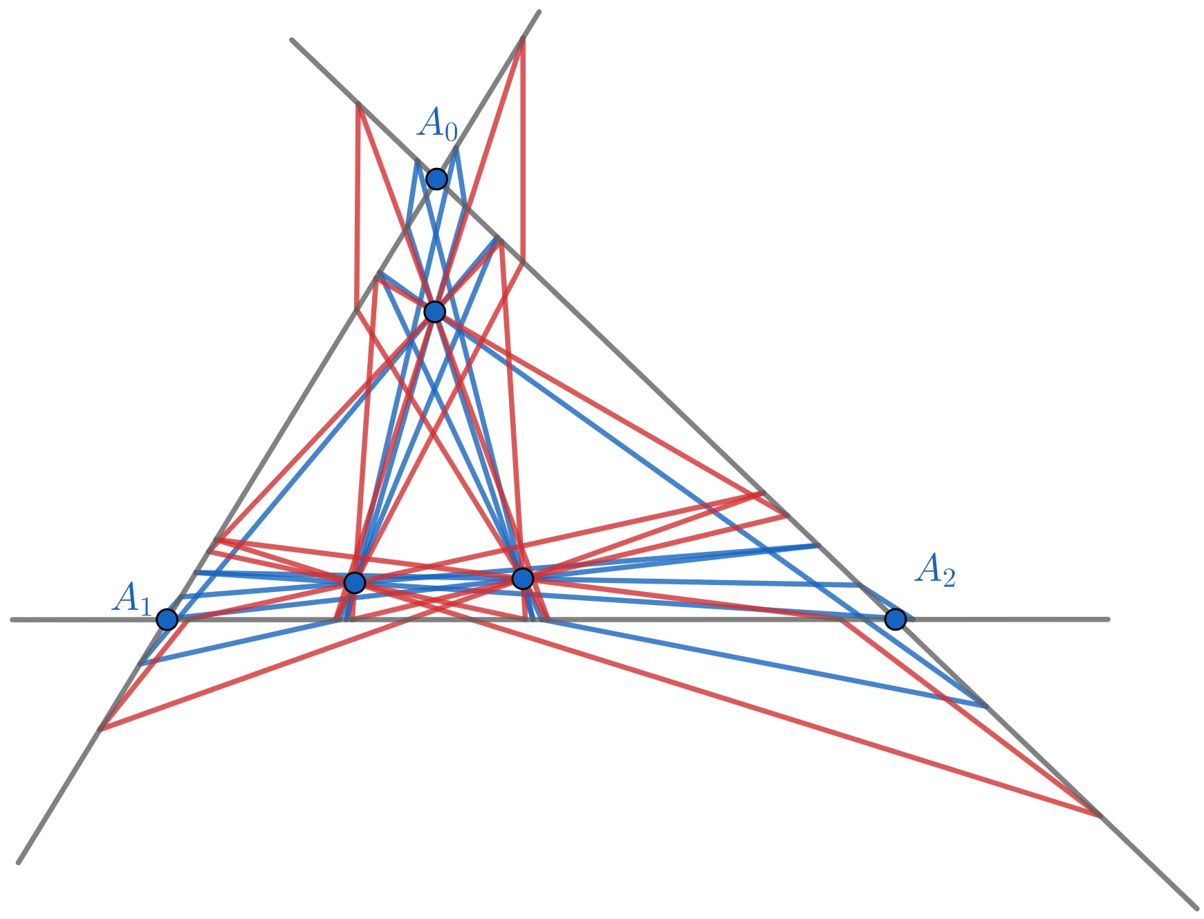
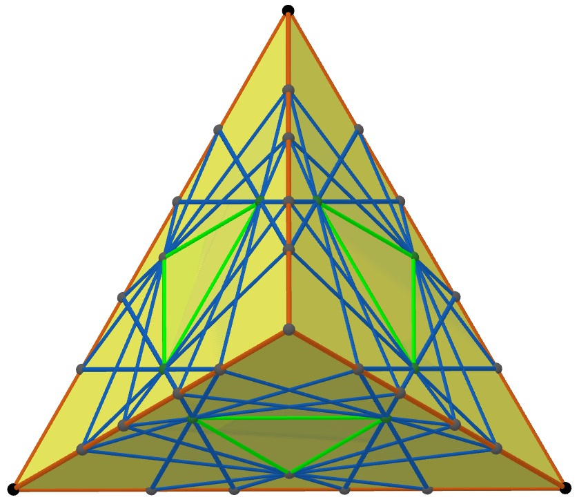
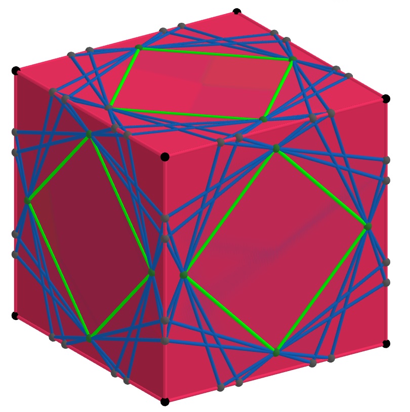
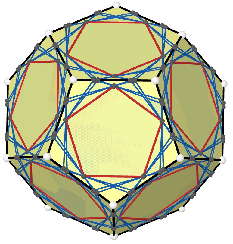
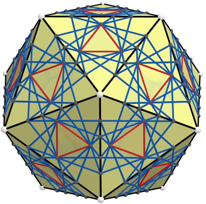
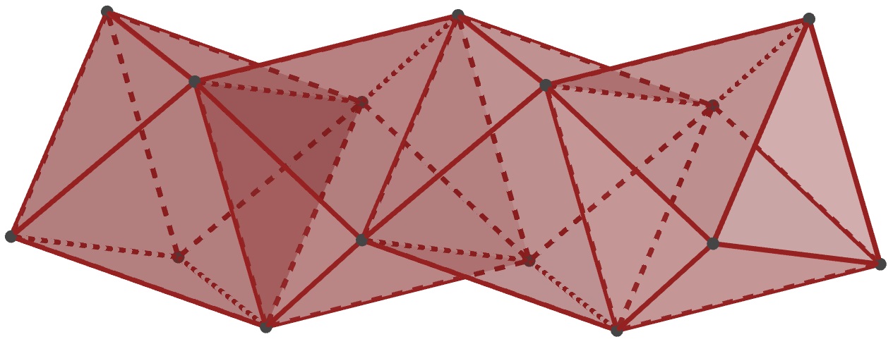
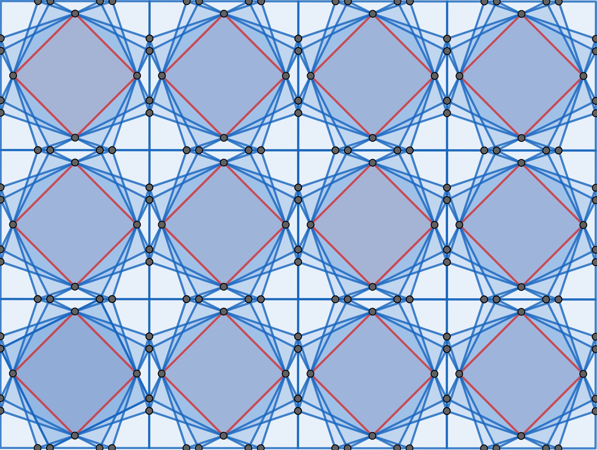
Let be a graph (vertices and edges) also called 1-skeleton ([18], p. 138) of a convex polyhedron. On each edge of choose a point which does not coincide with the vertices of . If the points on each polygonal face of are connected to form a convex polygon, then these polygons together form a graph, which we denote by (see Figure 1). In particular, if the number of faces meeting at each vertex of is 3 as in cube (see Figure 1), dodecahedron (see Figure 15), and tetrahedron (see Figure 13), then can also be interpreted as a convex polyhedron obtained by truncation of the vertices of the polyhedron of (see [11], Chapter 8). This means that in this case the convex hull of the vertices of form a convex polyhedron whose edges coincide with the edges of (see Figure 1). But if the number of faces meeting at some vertex of is greter than 3 as in octahedron (see Figure 2) and icosahedron (see Figure 16), then this interpretation is not possible, and therefore is just a graph. We say is inscribed into and similarly, is circumscribed around . Repeating this process for , we obtain its inscribed graph . The vertices of are chosen on the edges of one on each. Part of the edges of form convex polygons on the faces of . The remaining part of the edges of is not important to specify as they do not play any role in our considerations but for clarity we can assume them to connect only those 2 vertices of , which belong to 2 edges of having common vertex of and subtending angles on faces of with common vertex of . At each vertex of 4 edges and 4 faces are meeting and therefore interpretation of as a graph of a convex polyhedron obtained by truncation of the vertices of the polyhedron of is not always possible. Suppose now that graphs and are fixed. Is it possible to find graphs different from which are also inscribed into and circumscribed around , and if yes, then what is the maximum of their number? We will answer the second question by proving that this number can not exceed 4 and give an example of a convex polyhedron for which 4 such graphs exist (see Figure 2).
Note that all the edges of and all the vertices of are on the faces of . This means that the polygonal face of inscribed into a face of is also circumscibed around the polygonal face of lying on . All these faces are convex polygons and therefore we need to first solve the problem for the plane which has its own history and it is discussed in the next section.
2. Planar problem
Poncelet in his introduction to famous porism theorem, studied momentarily the variable polygons having all but one of their vertices on sides of a given polygon and all the sides passing through the vertices of another polygon. He shows that the free vertex describes a conic ([29], Tome I, p. 308-314). Poncelet cites Brianchon [6], who cites Maclaurin [24] and Braikenridge [5] for the case of triangles (see [25] for the history). Poncelet started to work on these questions in 1813 when he was a prisoner of war in Russia. In Poncelet porisms infinitude of polygons inscribed into one ellipse and and circumscribed around another ellipse, given that one such polygon exists, is proved [29], [30] (see also [7], [8], [20]). This result inspired discovery of many other porisms commonly known as Poncelet type theorems. In Steiner porism infinitude of chains of tangent circles all of which are internally tangent to one circle and externally tangent to another circle, again provided that one such chain exists, is studied (see[28], p.98; [10], sect. 5.8). In Emch’s porism Steiner’s porism is generalized to chain of intersecting circles, where these intersections are on another circle [16] (see also [2]). In Zig-zag type porisms infinitude of equilateral polygons with vertices taken alternately on two circles (or lines), is studied [4], [21], [14]. Money-Coutts theorem (see [33] and its references) is about chain of tangent circles alternately inscribed into angles of a triangle. Generalizations and connections of these results with each other, were studied in [3], [31], [15]. Similar generalizations for the space with rings of tangent spheres were discussed in [23], [9]. Surprisingly, the original configuration of Maclaurin about polygons inscribed into one polygon and circumscribed around another polygon did not attract much attention after these powerful generalizations. In the current section we will study in detail the case of convex polygons inscribed into one convex polygon and circumscribed around another one. The results are surprising as we will show that the maximal number of such polygons is not dependent on the number of sides of the polygons. At the end of Section 4 the case of generalized polygons, considered as collections of vertices or lines is also considered. Possibility of construction of such regular polygons with Euclidean instruments (straightedge and compass) is disscussed in Appendix A. This construction algorithm was very useful for drawing diagrams in the current paper all of which, except the last two, are created using the website of GeoGebra. For completeness we also provided an independent proof for generalized Maclaurin-Braikenridge’s conic generation method in Appendix B.
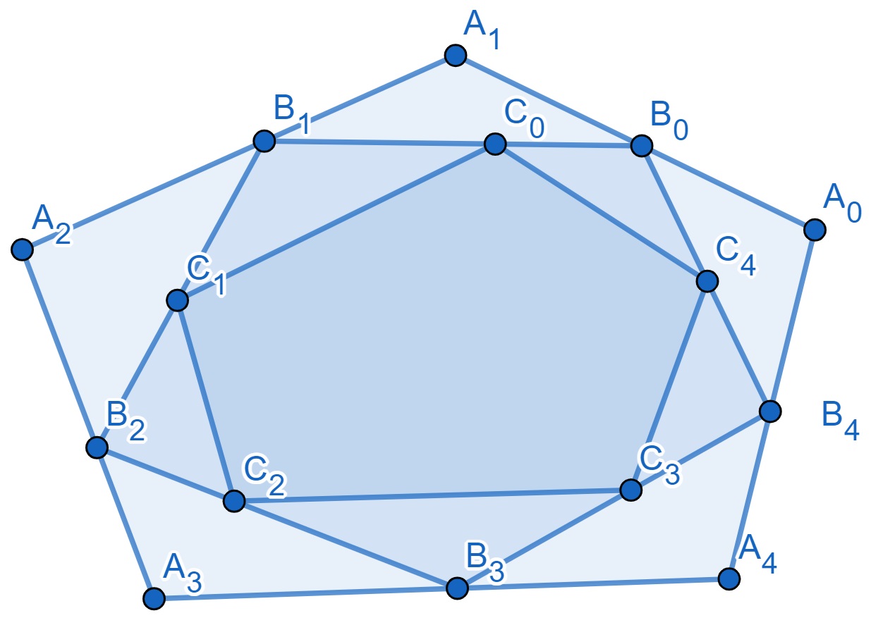
Suppose a convex polygon ) is given (see Figure 3). Choose a point on each side of this polygon. Denote these points by , where is between and , and . For such polygons we say that is inscribed into and is circumscribed around . In the same way choose on each side of polygon a point ( is between and , and for ) and draw polygon . Now fix polygons and . We want to find the maximum of the number of polygons like , which are inscribed into and circumscribed around , possibly with the indices shifted so that for some fixed . We will prove that this number is 4. Our strategy is to give an example where number 4 is realized and then prove that this number can not exceed 4.
The key ingredients of the proof will be the following examples and the lemma, which are interesting on their own.
Example 1.
Let be a regular polygon with with side length equal to and center . Let be the midpoints of . Let and denote . Then (see Fig. 4). Denote intersection point of line segments and by . Then
Denote One can check that
Therefore the two regular polygons corresponding to , and their reflections with respect to line form 4 polygons, which are inscribed into and circumscribed around . Note that points corresponding to and are constructible with compass and straightedge, provided that regular polygon is given (see Appendix A).
Example 2.
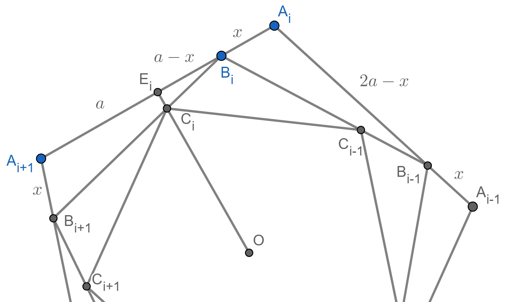
We will show how to find other exampes of 4 polygons inscribed into one and circumscribed around another convex polygon. Without loss of generality we can assume that (). We use notations similar to those from Example 1 (see Figure 5 for case ). Denote , , , , , where is the base of perpendicular from point to line for . We find that
By solving equation for we obtain
So, are the solutions of equation for . By changing and , we can get infinitely many examples for each (see Figure 5 and https://www.geogebra.org/calculator/exxbufdu). It would be useful to find that can work both for regular -gon and regular -gon, when . But we can show that it is impossible. Indeed, otherwise we would obtain
where is analogous distance for the -gon. By adding the corresponding equalities we would obtain
which is impossible because whenever .
Lemma 2.1.
Let cevians and of intersect at point . A line through point intersects line segments and at points and . Then .
Proof.
Let the line through point and parallel to line intersect line segments and at points and (see Figure 6). By Menelaus’ theorem
By similarity of and , and , and , we obtain . Finally, noting , we obtain
∎
Theorem 2.2.
The number of convex polygons , that can be inscribed into a given convex polygon and circumscribed around around another convex polygon is at most 4.
Proof.
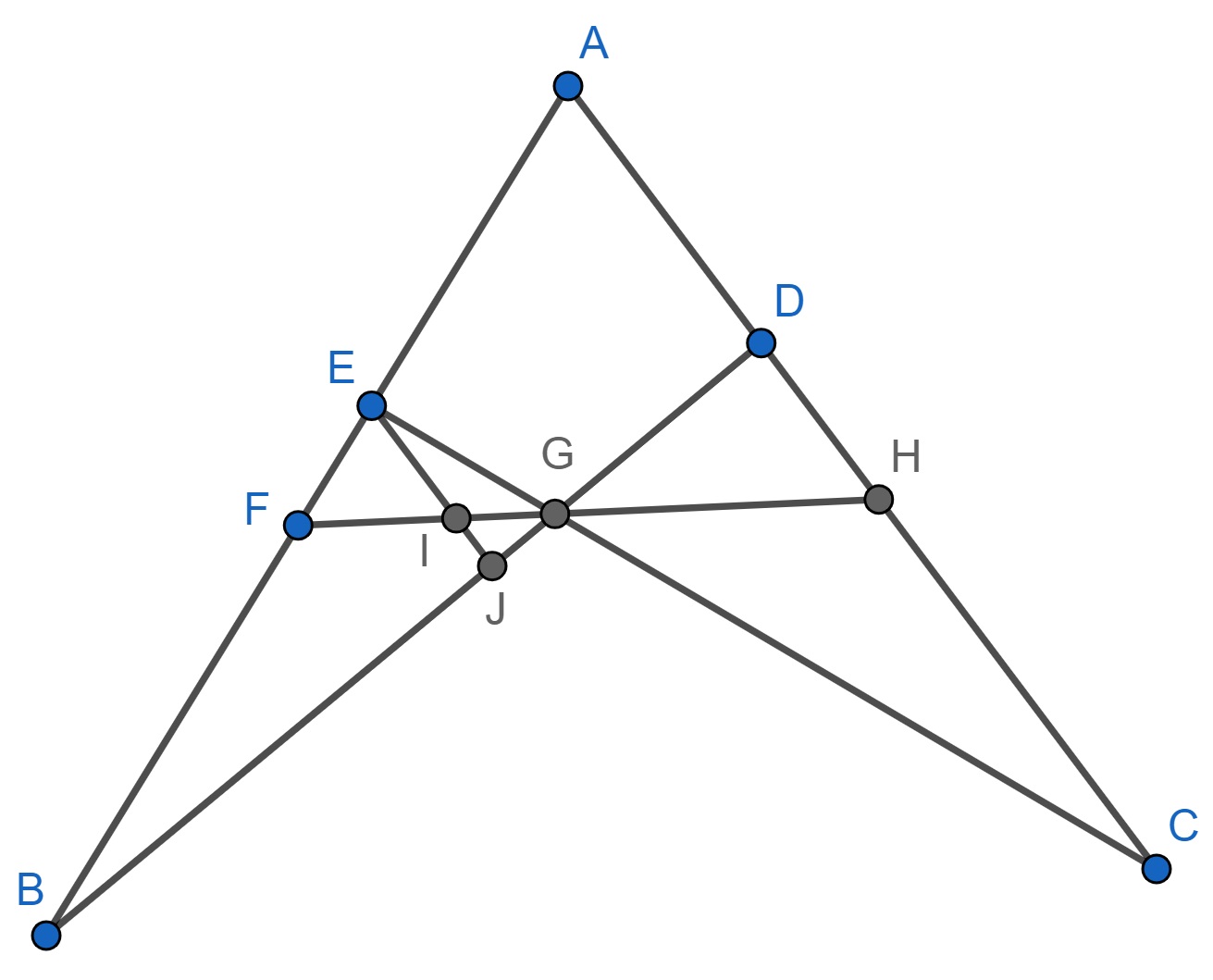
We saw in Example 1 (see also more general Example 2) that the case with 4 polygons is possible. Suppose on the contrary that there is a configuration with at least 5 polygons. Denote 5 of them by so that , for (see Figure 7). Immediately, , for all and . Consider the first two of the polygons: and . Then the vertices of are , where all the indices are taken modulo . Note that can not pass through . Indeed, otherwise pass through for all , and by Lemma 2.1,
for all , which is impossible, because it implies So, by convexity of and , passes through . This means that for . We can show that and are the only possible choices of for which (, and ). Indeed, if , then all sets
are disjoint (for only the interior regions of the triangles are considered) and . If , then the previous argument fails because coincides with and therefore . But if , then the only remaining option for is modulo 3, and this case is impossible because in this case there is such that , and therefore is closer to than , which is against our initial assumptions.
Consequently, , also pass through , and therefore , , and pass through for all . By Lemma 2.2,
for all , which is again impossible. This shows that our assumption about the existence of 5 polygons was wrong and therefore the maximal number of polygons is 4. ∎
Remark 2.3.
This result about convex planar polygons can be easily extended to convex polygons in spherical and hyperbolic geometry. Indeed, any convex spherical polygon is contained in a semisphere (see [17], Sect. 1.6) which can be projected centrally (also known as a gnomonic projection or rectilinear projection) to a plane resulting with convex planar polygons. Similarly, for hyperbolic geometry we can use Klein-Beltrami Model (see [22], Sect. 9.6, Fig. 226, 227).
Maclaurin-Braikenridge’s method.
3. Main results
We are now ready to answer the question about the maximum of the number of graphs inscribed into the graph of a convex polyhedron and circumscribed around another graph. As was mentioned before any such graph gives pattern of inscribed and circumscribed polygons on the faces of . By Theorem 2.2, their number can not exceed 4, which is the maximum of the number of convex polygons inscribed into one and circumscribed around another convex polygon. On the other hand we can give an example of a convex polyhedron with 4 inscribed graphs all of which are circumscribed around the same graph . As we take the graph of a regular octahedron all of the faces of which are equilateral triangles (see Firure 2). On each triangular face of the regular octahedron we construct 4 triangles as in Example 1 for . The vertices and the sides of these triangles on faces of octahedron give graph . The vertices of 8 inner triangles give the vertices of . Thus we proved the following result.
Theorem 3.1.
The number of graphs , that can be inscribed into graph of a given convex polyhedron and circumscribed around around another graph is at most 4.
Note that we can not apply the same method to tetrahedron and icosahedron to create another example similar to Figure 2, because at each vertex of the tetrahedron and icosahedron odd number of edges and faces meet (see Appendix C). Because of the odd number, in the resulting picture the vertices of will not alternate between closer and farther points on the edges of . Example 1 provides 4 polygons for any and therefore we can construct 4 squares or 4 pentagons as in the case of triangles. But for the same reason we can not use them on a cube and dodecahedron to create an example because again the number of edges meeting at each vertex is odd. There are of course semiregular polyhedra formed from 2 or more different regular polygons with equal sides. But in Example 2 we have shown that in a certain sense such an example with different polygons is impossible. Nevertheless this does not exclude the possibility of more general examples.
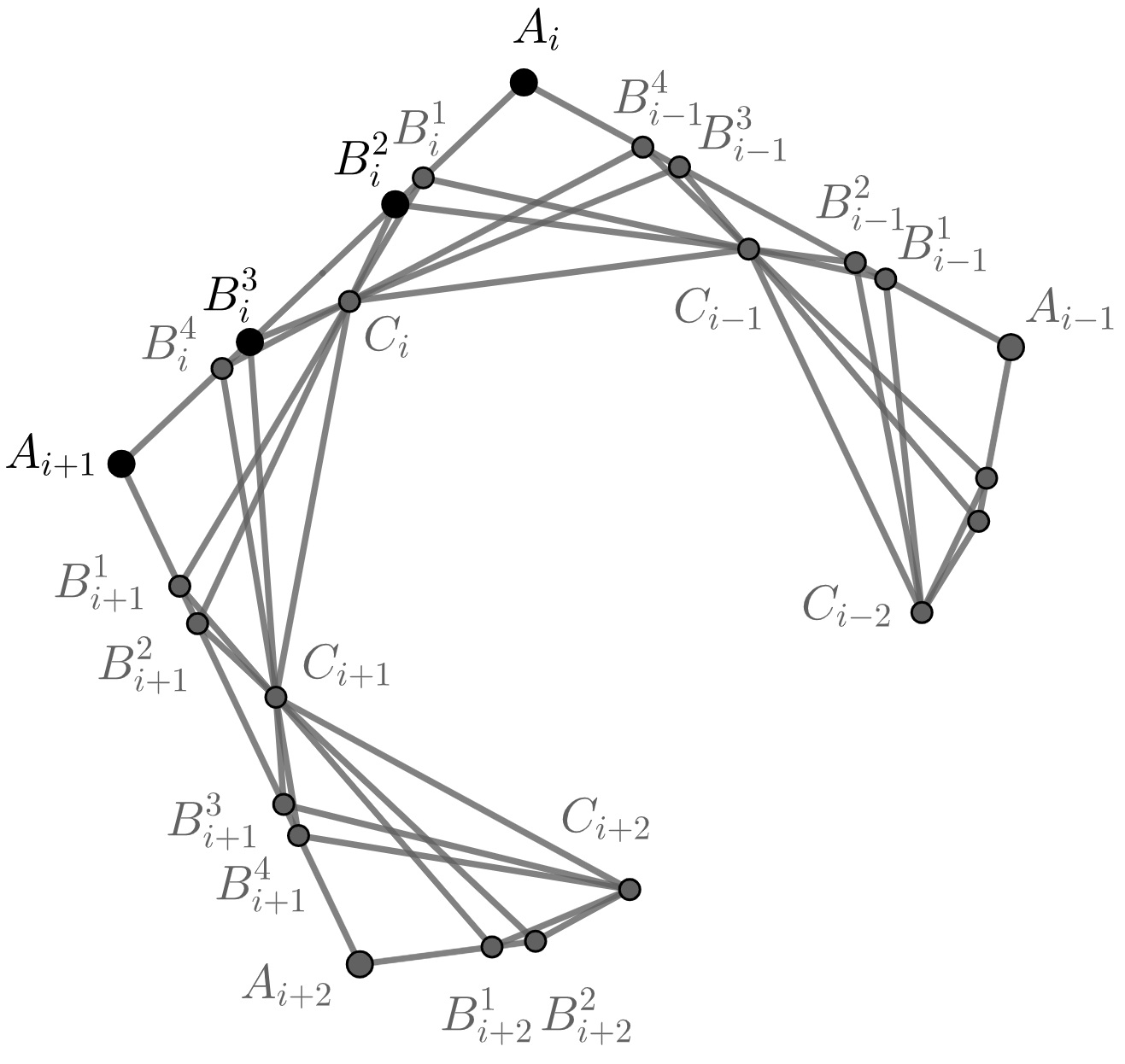
By combining several octahedra together on their triangular faces, so that any vertex belongs to only 1 or 2 octahedra, one can construct arbitrarily large polyhedra which can serve as non-convex examples for Theorem 3.1 (see Appendix C). It would be interesting to generalize these results and their proofs for higher dimensions. Beside the question about higher dimensions several other questions can be asked for further exloration.
Problem 1.
Is it always possible to inscribe 4 convex polygons into any given convex polygon so that all 4 are circumscribed around another convex polygon?
Problem 2.
Is it always possible to inscribe 4 graphs into graph of any given convex polyhedron so that all 4 are circumscribed about another graph?
Problem 3.
Is the octahedron and its inscribed graphs in Figure 2 the only example of this kind for Platonic regular and Archimedes’ semi-regular polyhedra?
Problem 4.
What can be said about the number of inscribed/circumscribed convex polyhedra obtained by the process of truncation of their vertices?
Problem 5.
What can be said about the number of face-inscribed/circumscribed convex polyhedra?
4. Maclaurin-Braikenridge’s method of conic generation
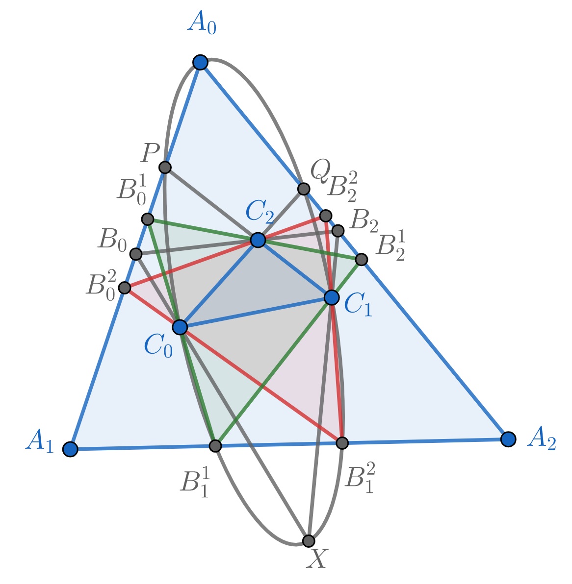
It is well known that if triangles and are given, moving line passes through , where and are on lines and , respectively, then the locus of intersection point of and is in general a conic (see Figure 8). See e.g. [32], p. 230, [26], p. 22, [27], p. 97, [36], [28], p. 328, where this result, known as Maclaurin-Braikenridge’s method of conic generation, is generalized for polygons and . If , then this conic passes through and , where and . This conic can intersect at maximum 2 points shown in Figure 8 as and , which can be starting point for the construction of 2 triangles and inscribed into and circumscribed around . Therefore the key argument of using Lemma 2.1 in the proof of Theorem 2.3, can also be replaced by the fact that a general conic and a line can intersect at maximum 2 points.
Also, an important and natural connection to projective geometry can be mentioned. The problem can be reformulated as finding fixed points of a projective transformation of a line. Indeed, let be the central projection with center from the line to the line . The polygon is a solution to the problem if and only if . A projective transformation either has at most two points or is the identity (Von Staudt’s lemma, see e.g. [19], p. 79), therefore the problem can have 0, 1, 2 or many solutions when the shift is fixed. Thus the proof of Theorem 2.2 actually shows that this projective transformation is not the identity, under certain assumptions on the position of lines and projection centers. In any case, it is not difficult to see that the projective transformation of obtained by taking these central projections cannot be an identity because is not a fixed point. If it were, then would have to be on the line since is on that line and must go through . Note the fact that 2 of the 4 polygons correspond to one projective transformation and the other 2 correspond to another one. There is a shift in the index which was mentioned in Section 2.
The generalization of Maclaurin-Braikenridge’s method was studied through analytic tools in [29], Tome I, p. 308-314 (see [6] for geometric consideration). The proof of case is the converse of Pascal’s theorem [10], which states that hexagon is inscribed into a conic ([34], p.321, [35], p. 377). The general case can be proved by induction on (see Section 5). Using this general result it is possible to show that if the condition of convexity is lifted and the polygons are extended to include also the lines containing the sides of the polygons, then in the general case, the maximal number of polygons inscribed into one polygon and circumscribed around another one, can be as large as (excuding degenerate cases when the conics can coincide with the lines giving infinitely many such polygons [29], Tome 2, p. 10, [27], p. 97). Indeed, there are cyclic permutations of the sides of polygon . Between these sides the vertices of polygon can be put in ways. Because of independence, we multiply them to obtain , then divide by 2 (orientation is not important) and finally multiply by 2 (each conic gives at most two polygons) to obtain again . For example, if , then there are at most 12 triangles, all of which are shown in Fig. 7.
Construction of (https://www.geogebra.org/geometry/jjxzgu7a).
Appendix A: Construction with straightedge and compass
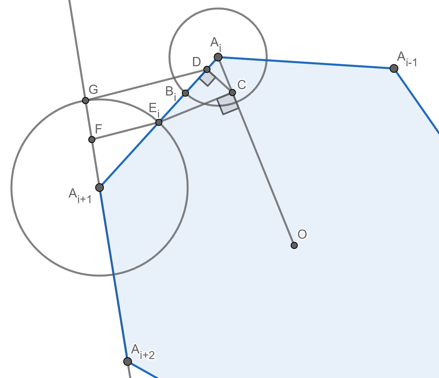
Suppose that regular polygon is given. Note that point corresponding to is the midpoint of , which is easy to construct using unmarked ruler and compass. Below we will show how to construct using the same instruments point corresponding to . If , then , and its construction is straightforward. So, we assume that . Let be, as before, the midpoint of side of regular polygon .
-
(1)
Drop perpendicular to line .
-
(2)
Drop perpendicular to line .
-
(3)
Draw circle with center through . Let this circle intersect line outside of line segment at point .
-
(4)
Draw line through parallel to . Let this line intersect line at point .
-
(5)
Draw circle with center and radius equal to through . This circle intersect line segment at point such that .
The proof follows from the following arguments. Note first that , where as before . Then and therefore . Since ,. Also from similarity of and we obtain that , which simplifies to . If , then there is a shorter construction based on the fact that the corresponding sides of triangles and are parallel (see Figure 2). Similarly, if , then one can use the fact that .
Note also that if regular polygon and point with specific is given, then one can construct using the same instruments another point with , such that Indeed, is the second solution of quadratic equation (the first solution is ), all of the coefficients of which are constructible. For , one can check that .
Appendix B: Generalized Maclaurin-Braikenridge’s conic generation
In this part of the paper an independent proof of generalized Maclaurin-Braikenridge’s theorem for -gons will be given. It is based on the method of mathematical induction for . First, we need to prove the following lemma.
Lemma 4.1.
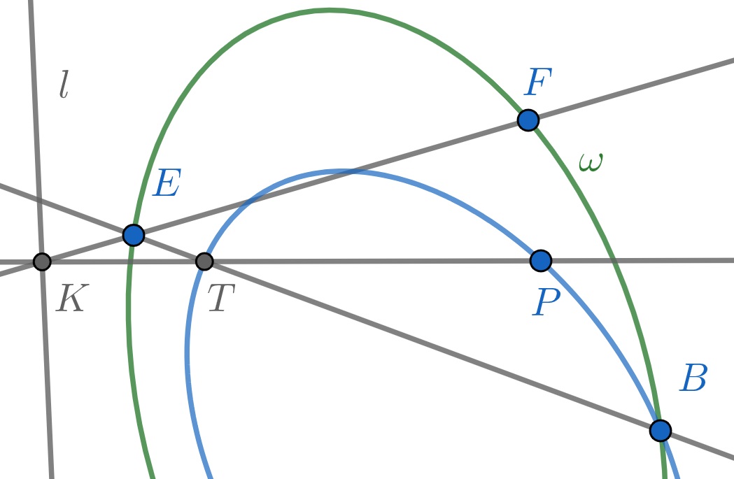
Let fixed points and , and moving point be on a given conic . Let and be a given point and a given line on the plane of . Let intersect at point , and intersect at . Then the locus of point is a conic passing through points and (see Fig. 9).
Proof.
Consider 2 cases.
Case 1. Suppose that line does not intersect conic . Then we can apply a projective transformation mapping to infinite line and then an affine transformation mapping the image of conic to a circle. Let us use the same letters for the new objects. When changes on circle , does not change. Since is now an infinite point on infinite line , , and therefore, . So, locus of is a circle. This means that inverse of affine and projective transformations of the locus of will be a conic.
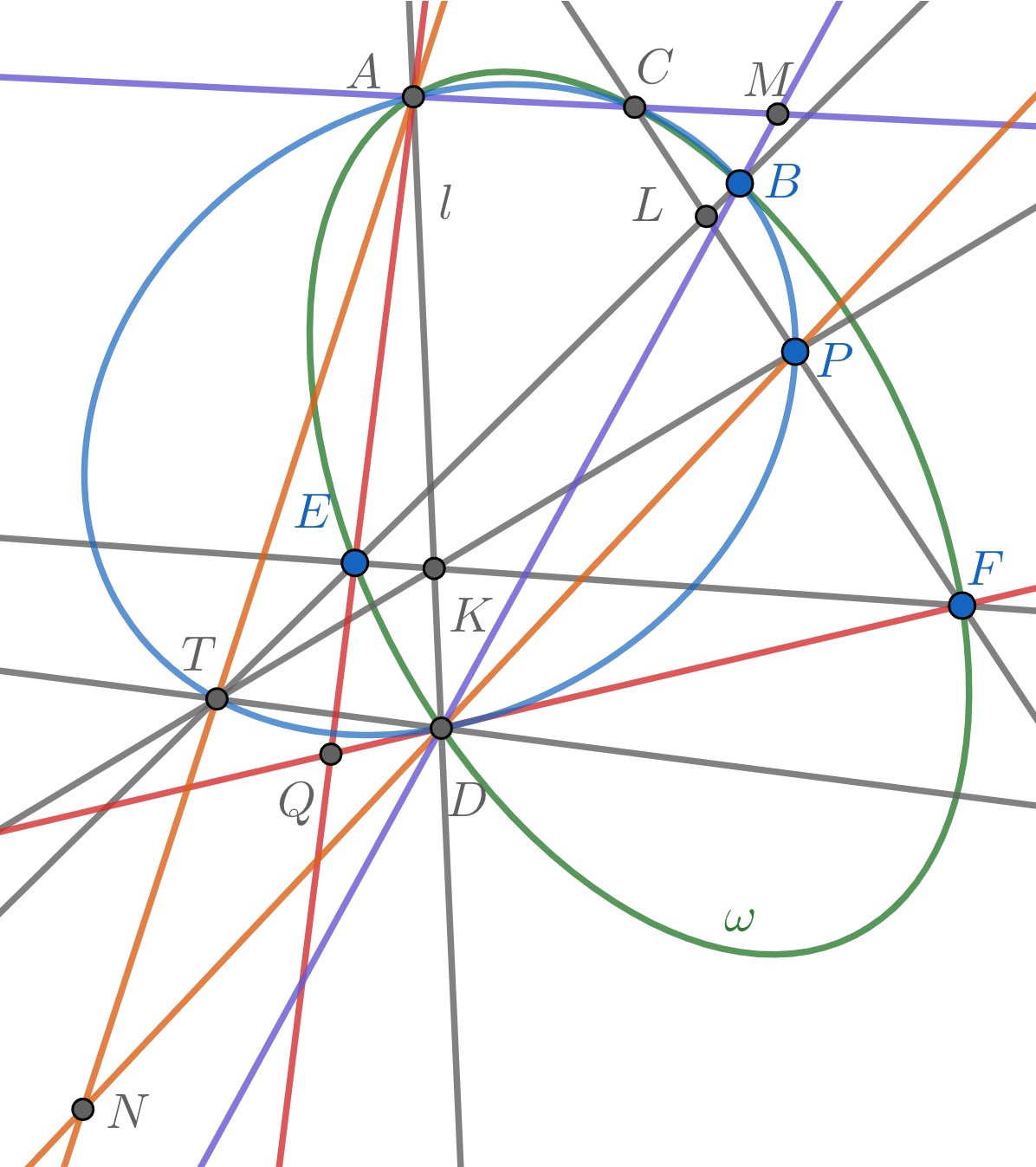
Case 2. Suppose now that intersects at points and as in Fig. 10. Denote , , , , and . By Pascal’s theorem, since hexagon is inscribed into conic , points are collinear. By Desarques’ theorem, since and are perspective with respect to point (, , and are concurrent), these triangles are also perspective with respect to a line. Therefore points , , and are collinear. Then by Pascal’s theorem, hexagon is inscribed into a conic. Since points are fixed, the locus of point is a conic. ∎
We are ready to state and prove the following general result.
Theorem 4.2.
Let be lines, and be points in general position . Let changing points and be chosen so that . Then the locus of point is a conic passing through and .
Proof.
We saw in Section 4 that the case is the converse of Pascal’s theorem and therefore it is easily proved [12], p. 85. Suppose that the claim is true for , which means that the locus of is a conic passing through and . If we take in Lemma 5.1 , , , , , , , , then we obtain that the locus of is a conic passing through and . ∎
As in Section 4 above Projective geometry provides a two-lines but non-elementary proof of the generalized Maclaurin-Braikenridge conic generation. The map sending the line to the line in Theorem 5.2 is a projective map between two pencils of lines, and by the Steiner’s conic generation (see e.g. [19], p. 178) the intersection point of such projectively related lines traces a conic.
Appendix C: Other Platonic solids and non-convex polyhedra.
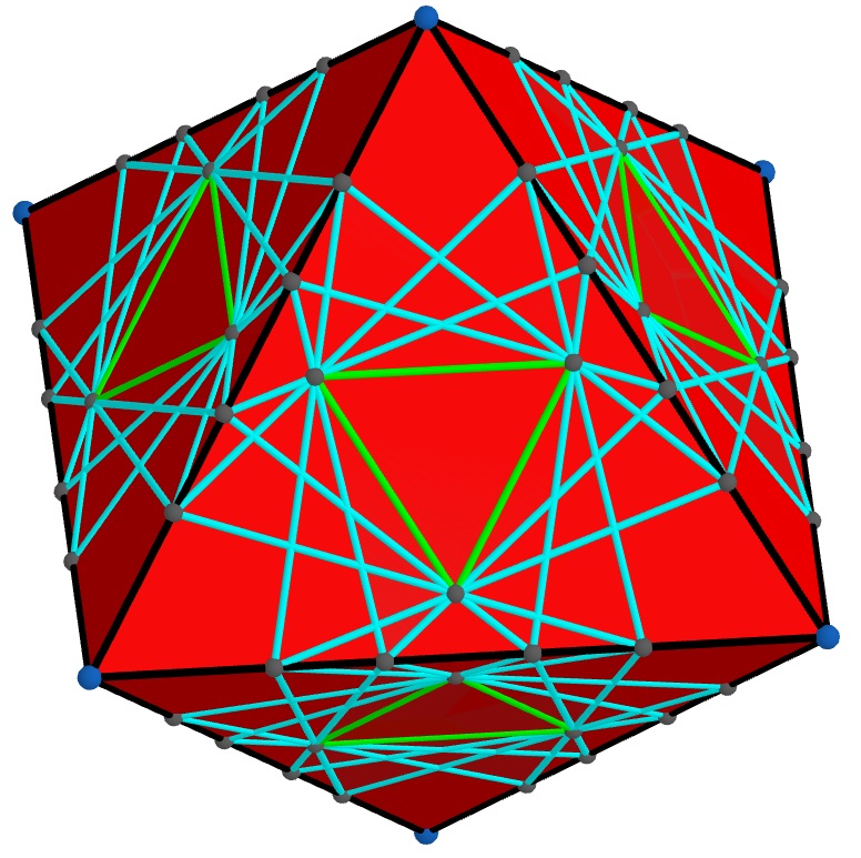
Figures 13-16 show 4 remaining Platonic solids which enjoy many symmetries but do not give an example for Theorem 3.1 because of odd number of faces meeting at each vertex. It would be interesting to determine if for 4 dimensions analogous regular polytopes give an example of 4 inscribed/circumscribed graphs or not.
There are also non-convex polyhedra for which it is possible to construct an example similar to Figure 2. In Figure 17 several octahedra are joined along their triangular faces so that at each vertex only 4 or 6 faces meet. One can increase the number of octahedra to obtain arbitrarily large such non-convex examples. In Figure 18 and Figure 19, you can see models of non-convex polyhedra with 10 vertices, 24 edges, and 16 triangular faces, and 11 vertices, 27 edges, and 18 triangular faces, respectively, made of Geomag pieces. Note that at each vertex of these polyhedra again 4 or 6 faces meet, which make it possible to construct examples similar to the octahedron in Figure 2.
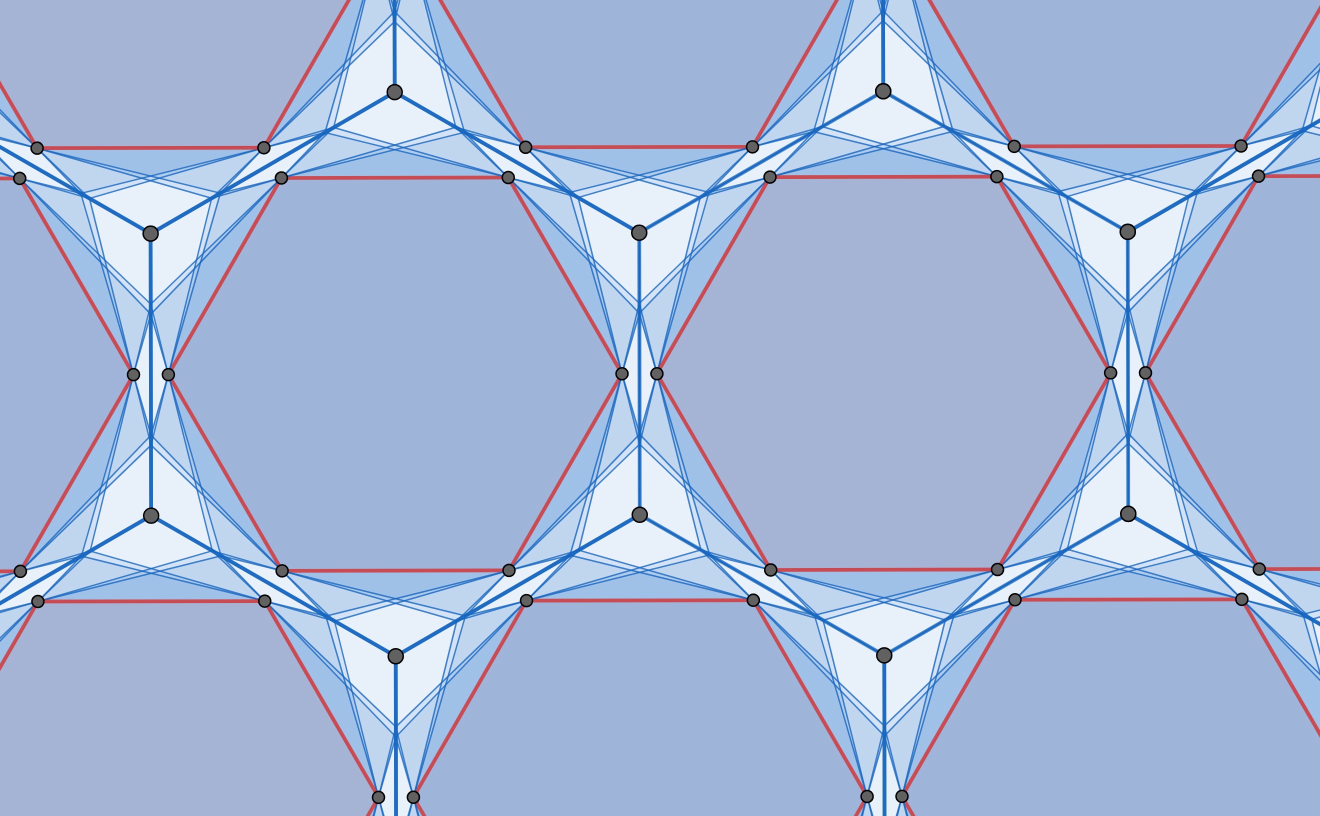
Planar grids formed by regular hexagons, squares and triangles can be interpreted as infinitely large (degenerate) polyhedra (see [17], Sect. 1.7). In the case of hexagons (Figure 20) odd number of faces meet at each vertex, but for squares (Figure 21) and triangles this number is even. For this reason, hexagons do not give examples similar to Fig. 2, but squares and triangles do.
5. Conclusion
In the paper the question about the maximum of the number of graphs inscribed into the graph of a convex polyhedron and circumscribed about another graph, is discussed. The maximal number of such graphs is shown to be 4. Constructible examples of these 4 graphs (convex polygons) in the case of regular icosahedron (regular polygon) are given. The special problem for convex polygons on a plane is also solved. The connection with projective geometry, generalized Maclaurin-Braikenridge’s conic generation method and its new proof based on mathematical induction are also included.
Acknowledgments
6. Declarations
Ethical Approval.
Not applicable.
Competing interests.
None.
Authors’ contributions.
Not applicable.
Funding.
This work was completed with the support of ADA University Faculty Research and Development Fund.
Availability of data and materials.
Not applicable
References
- [1]
- [2] E.A. Avksentyev, The Great Emch Closure Theorem and a combinatorial proof of Poncelet’s Theorem, Mat. Sb., 206:11 (2015), 3–18; Sb. Math., 206:11 (2015), 1509–1523. https://doi.org/10.1070/SM2015v206n11ABEH004503
- [3] Th. Bauer, W. Barth, Poncelet theorems. Exposition. Math. 14, (1996) 125-144.
- [4] O. Bottema, Ein Schliessungssatz für zwei Kreise, Elem. Math. 20:1 (1965), 1–7.
- [5] W. Braikenridge, Exercitatio Geometrica de Descriptione Curvarum, London, 1733.
- [6] M. Brianchon, Solution de plusieurs problèmes de géométrie, Journal de l’École polytechnique, IX Cahier., Tome IV, 1810, 1-15. https://gallica.bnf.fr/ark:/12148/bpt6k433667x/f2.item
- [7] A. Del Centina, Poncelet’s porism: a long story of renewed discoveries, I. Arch. Hist. Exact Sci. 70, 1–122 (2016). https://doi.org/10.1007/s00407-015-0163-y
- [8] A. Del Centina, Poncelet’s porism: a long story of renewed discoveries, II. Arch. Hist. Exact Sci. 70, 123–173 (2016). https://doi.org/10.1007/s00407-015-0164-x
- [9] Coxeter, H.S.M. Interlocking Rings of Spheres. Scripta Math. 18, 113-121, 1952.
- [10] H.S.M. Coxeter, S.L. Greitzer, Geometry revisited, Series: New mathematical library 19, Mathematical Assoc. of America, 2008.
- [11] Coxeter, H.S.M. Regular Polytopes, (3rd edition, 1973), Dover edition.
- [12] H.S.M. Coxeter, Projective Geometry, Springer, New York, 1987.
- [13] P.R. Cromwell, Polyhedra, Cambridge University Press; 1st edition (1999).
- [14] B. Csikós, A. Hraskó, Remarks On The Zig-zag Theorem, Periodica Mathematica Hungarica 39, (2000) 201–211. https://doi.org/10.1023/A:1004811527911
- [15] V. Dragović, M. Radnović, Poncelet Porisms and Beyond, Integrable Billiards, Hyperelliptic Jacobians and Pencils of Quadrics, Birkhäuser, Basel, 2011. https://doi.org/10.1007/978-3-0348-0015-0
- [16] A. Emch, An Application of Elliptic Functions to Peaucellier’s Link-Work (Inversor). Annals of Mathematics, 2(1/4), (1900) 60–63. https://doi.org/10.2307/2007182
- [17] L. Fejes Tóth, G. Fejes Tóth, W. Kuperberg, Lagerungen Arrangements in the Plane, on the Sphere, and in Space, Grundlehren der mathematischen Wissenschaften Series 360, Springer, 2023. https://doi.org/10.1007/978-3-031-21800-2
- [18] Grünbaum, Branko. Convex Polytopes, Graduate Texts in Mathematics, vol. 221 (2nd ed.), Springer-Verlag (2003).
- [19] G.B. Gurevich, Projective geometry, Fizmatgiz, Moscow (1960) (in Russian).
- [20] L. Halbeisen, N. Hungerbühler. (2015). A Simple Proof of Poncelet’s Theorem (on the Occasion of Its Bicentennial). The American Mathematical Monthly, 122(6), 537–551. https://doi.org/10.4169/amer.math.monthly.122.6.537
- [21] A. Hraskó, Poncelet-type Problems, an Elementary Approach. Elem. Math. 55 (2000), no. 2, 45–62. https://doi.org/10.1007/s000170050071
- [22] Klein, F., Rosemann, W., Vorlesungen über nicht-euklidische Geometrie, Springer, Berlin 1968. http://resolver.sub.uni-goettingen.de/purl?PPN375534636
- [23] L. Kollros, Quelques théorèmes de géométrie. Commentarii mathematici Helvetici 11 (1938/39): 37-48. http://eudml.org/doc/138715
- [24] C. MacLaurin, A Letter from Mr. Colin Mac Laurin, Math. Prof. Edinburg. F.R.S. to Mr. John Machin, Ast. Prof. Gresh. & Secr. R.S. concerning the Description of Curve Lines’, Phil. Trans. 39 (1735-36), 143-165.
- [25] S. Mills, Note on the Braikenridge-Maclaurin Theorem. Notes and Records of the Royal Society of London, 38(2), (1984) 235–240. http://www.jstor.org/stable/531819
- [26] P. Pamfilos, Circles Associated To Pairs Of Conjugate Diameters, International Journal Of Geometry, Vol. 7 (2018), No. 1, 21 - 36.
- [27] P. Pamfilos, On the Newton Line of a Quadrilateral, Forum Geometricorum, Vol. 9 (2009) 81–98.
- [28] D. Pedoe, Geometry: A Comprehensive Course, Dover, New York, 1988.
- [29] J.V. Poncelet, Applications d’ analyse et de geometrie, Gauthier-Villars, in 2 vol. 1864 (1964). Tome I: https://gallica.bnf.fr/ark:/12148/bpt6k90213q/f324.item.texteImage Tome II: https://gallica.bnf.fr/ark:/12148/bpt6k97644068/f24.item.texteImage
- [30] J.V. Poncelet, Traité des propriétés projectives des figures, Gauthier-Villars, Paris, 1865. https://gallica.bnf.fr/ark:/12148/bpt6k9608143v/
- [31] V.Yu. Protasov, A generalization of Poncelet’s theorem, Russian Mathematical Surveys, 2006, Volume 61, Issue 6, 1180–1182. https://doi.org/10.1070/RM2006v061n06ABEH004375
- [32] G. Salmon, A treatise on conic sections, Longmans, London, 1855.
- [33] S. Tabachnikov, Going in Circles: Variations on the Money-Coutts Theorem. Geometriae Dedicata 80, 201–209 (2000). https://doi.org/10.1023/A:1005204813246
- [34] H.W. Turnbull, Colin Maclaurin, The American Mathematical Monthly, 54:6, (1947) 318-322. https://doi.org/10.1080/00029890.1947.11991846
- [35] I. Tweddle, The Prickly Genius: Colin MacLaurin (1698-1746). The Mathematical Gazette, 82(495), (1998) 373–378. https://doi.org/10.2307/3619883
- [36] C. R. Wylie, Some Remarks on Maclaurin’s Conic Construction, Mathematics Magazine, 1968, Vol. 41, No. 5, 234-242. https://www.jstor.org/stable/2688802
- [37]