The Ordered Zeckendorf Game
Abstract.
We introduce and analyze the ordered Zeckendorf game, a novel combinatorial two-player game inspired by Zeckendorf’s Theorem, which guarantees a unique decomposition of every positive integer as a sum of non-consecutive Fibonacci numbers. Building on the original Zeckendorf game—previously studied in the context of unordered multisets—we impose a new constraint: all moves must respect the order of summands. The result is a richer and more nuanced strategic landscape that significantly alters game dynamics.
Unlike the classical version, where Player 2 has a dominant strategy for all , our ordered variant reveals a more balanced and unpredictable structure. In particular, we find that Player 1 wins for nearly all values , with a single exception at . This shift in strategic outcomes is driven by our game’s key features: adjacency constraints that limit allowable merges and splits to neighboring terms, and the introduction of a switching move that reorders pairs.
We prove that the game always terminates in the Zeckendorf decomposition—now in ascending order—by constructing a strictly decreasing monovariant. We further establish bounds on game complexity: the shortest possible game has length exactly , where is the number of summands in the Zeckendorf decomposition of , while the longest game exhibits quadratic growth, with as .
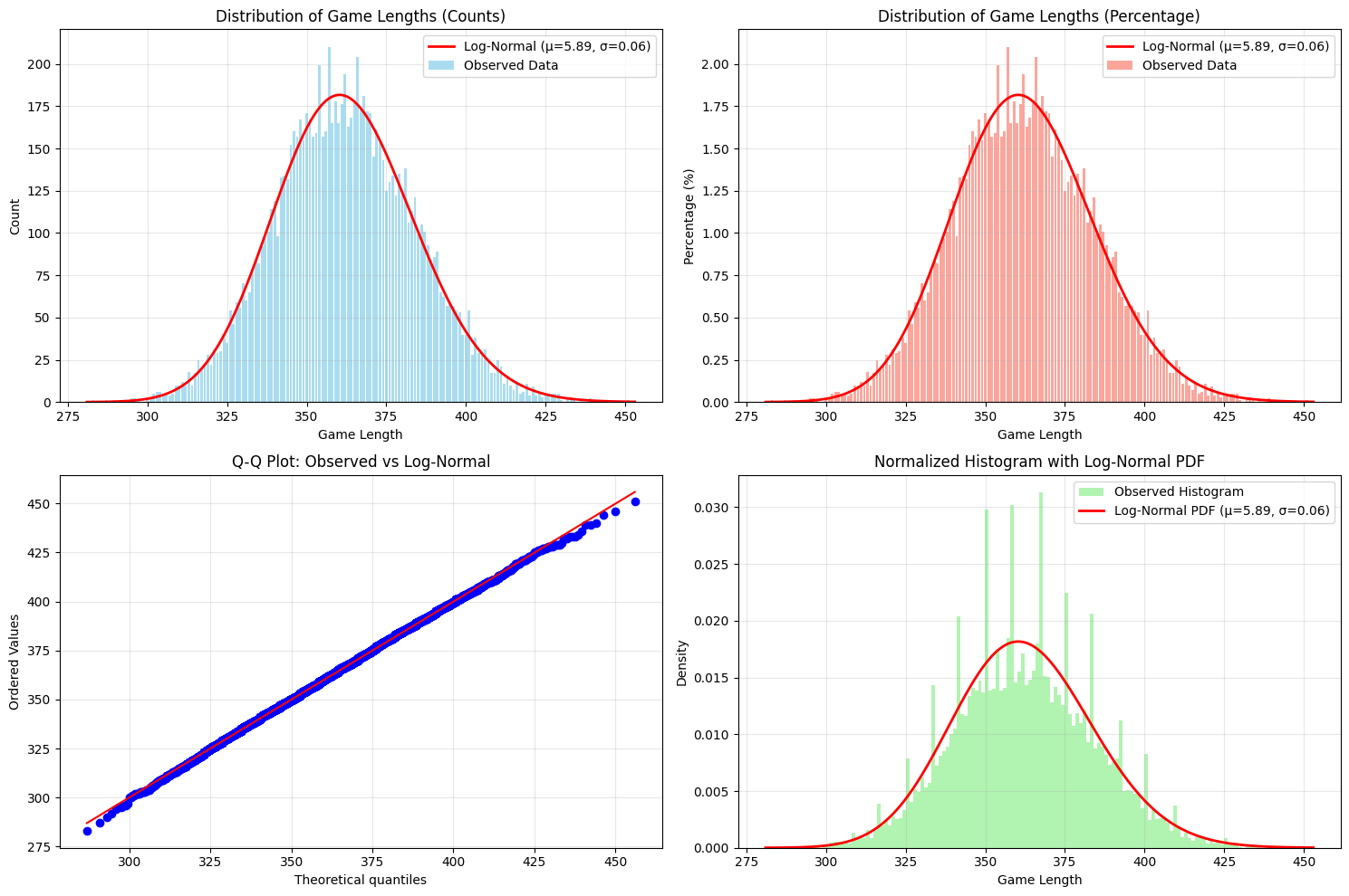
Empirical simulations suggest that random game trajectories exhibit log-normal convergence in their move distributions. Overall, the ordered Zeckendorf game enriches the landscape of number-theoretic games, posing new algorithmic challenges and offering fertile ground for future exploration into strategic complexity, probabilistic behavior, and generalizations to other recurrence relations.
Key words and phrases:
Fibonacci numbers, Zeckendorf’s Theorem, Zeckendorf Games1. Introduction
1.1. History and Motivation
The Fibonacci sequence is given by , and for . Zeckendorf’s Theorem [9] states that every positive integer can be uniquely represented as a sum of non-consecutive Fibonacci numbers, noting that in order to guarantee uniqueness it is necessary that we have only one term equal to . This decomposition can be efficiently obtained via a greedy algorithm, and its structural and probabilistic properties have been extensively investigated across combinatorics, number theory, and discrete mathematics. A game-theoretic interpretation of the theorem was first proposed in [1], where two players alternately perform legal replacements on a multiset of Fibonacci numbers until reaching the unique Zeckendorf decomposition. A formal definition of the classical Zeckendorf Game is given below.
Definition 1.1 (The Two Player Zeckendorf Game).
At the beginning of the game, there is an unordered list of 1’s: . Players alternate turns, and on each turn, a player may make one of the following moves.
-
(1)
Merging: Replace with .
-
(2)
Merging Ones: Replace with .
-
(3)
Splitting: Replace with for .
-
(4)
Splitting Twos: Replace with .
The game ends when no further moves can be made.
In the classical Zeckendorf game, the order of summands is irrelevant—players operate on unordered collections of Fibonacci numbers, applying merge or split operations regardless of position. It is known that in this formulation, Player 2 has a winning strategy for all , which significantly limits the strategic complexity of the game [2].
To address these limitations and explore deeper combinatorial structures, we introduce a new variant: the ordered Zeckendorf game. In our version, the game begins with an ordered -tuple of , and all allowed moves are restricted to adjacent elements. The resulting dynamics differ significantly from those in the unordered setting, as adjacency constraints restrict player choices and emphasize positional strategy. Remarkably, we find that for all —with the sole exception of , where Player 2 has a winning strategy—Player 1 can force a win. This is in sharp contrast to the classical game and suggests that the introduction of order restores balance and increases strategic depth.
Our variant introduces a novel move: the switch, which allows players to swap adjacent elements out of order. This rule further enhances the game’s complexity, producing larger game trees and requiring careful local planning. The interaction between merging, splitting, and switching operations creates a rich environment for strategic exploration, raising new algorithmic and theoretical questions.
This paper presents a comprehensive analysis of the ordered Zeckendorf game, combining theoretical results with computational observations. We prove that every game terminates in the ascending Zeckendorf decomposition of , using a carefully constructed monovariant. We also establish lower and upper bounds on game length and propose a conjectural strategy for maximizing the number of moves. Finally, we investigate the distribution of random play lengths and observe evidence suggesting convergence to a log-normal distribution.
Our work contributes to an expanding literature on Zeckendorf-type games and generalized decompositions. For readers seeking additional context or further directions, we recommend the following references:
-
•
Beckwith et al. [3], on average gap distributions in generalized Zeckendorf decompositions,
-
•
Kopp et al. [7], on the number of summands in Zeckendorf decompositions,
-
•
Gueganic et al. [6], on limiting distributions in generalized settings,
-
•
Baird-Smith et al. [2], on the generalized Zeckendorf game,
-
•
Boldyriew et al. [4], on extensions to non-constant recurrence relations,
-
•
Cusenza et al. [5], on multiplayer and alliance-based Zeckendorf games.
1.2. Main Results
We use to denote the Fibonacci number, where , , and the recurrence relation holds for all .
Definition 1.2 (The Two-Player Ordered Zeckendorf Game).
At the start of the game, the state is an ordered list of copies of : . Players alternate turns, and on each turn, a player may perform one of the following five legal moves.
-
(1)
Merging: Replace a pair of adjacent terms with .
-
(2)
Merging Ones: Replace with .
-
(3)
Splitting: Replace a pair with , for .
-
(4)
Splitting Twos: Replace with .
-
(5)
Switching: Swap adjacent elements whenever .
The game ends when no further moves can be applied; that is, when the list of Fibonacci numbers is strictly increasing and no merge or split move is possible.
These sum-preserving operations derive naturally from the Fibonacci recurrence and the constraints imposed by ordering. Merges and splits allow construction and deconstruction of Fibonacci terms, while switches restore ascending order to enable further operations. Together, they encode a localized, combinatorial decision-making framework that is both computationally rich and strategically deep.
Our main theoretical results fall into three broad categories: termination and correctness of the game, bounds on its length, and structural conjectures about optimal play.
Theorem 1.3 (Termination and Final State).
The ordered Zeckendorf game always terminates in a finite number of moves. Moreover, the final state is the Zeckendorf decomposition of , expressed as a strictly increasing sequence of Fibonacci numbers.
The proof of this result proceeds by defining a suitable monovariant that decreases strictly with each move. The monovariant simultaneously tracks disorder (via inversions) and total weight (via the sum of Fibonacci indices), ensuring that the game cannot cycle and must converge. Importantly, the final configuration must be the unique Zeckendorf decomposition, as all alternative representations are eliminated by the move set. Since the game always terminates in a unique configuration, we can define natural extremal questions: What is the minimal number of moves required? What is the maximum? We begin with the lower bound.
Proposition 1.4 (Shortest Game).
The shortest possible game has length , where is the number of terms in the Zeckendorf decomposition of .
This minimal length corresponds to a greedy strategy in which players always combine adjacent pairs as quickly and effectivelly as possible to reach the final state with minimal intermediate steps.
At the other extreme, we are interested in how long the game can be prolonged under optimal play designed to delay termination.
Theorem 1.5 (Upper Bound on the Maximal Game Length).
Let denote the maximal length of the Ordered Zeckendorf game on . Then
To complement this upper bound, we provide a lower bound for by proposing a specific strategy that aims to maximize the game length.
Definition 1.6 (Long Game Strategy).
The Long Game Strategy (LGS) is defined as the following priority-based strategy.
-
(1)
Perform switch moves (in any order).
-
(2)
Combine adjacent ones, starting from the left.
-
(3)
Perform split moves, starting from the right.
-
(4)
Perform merge moves, starting from the left.
Conjecture 1.7 (Strategy for Maximum Length).
The LGS has the longest game length.
This conjecture is supported by exhaustive simulations, providing strong empirical evidence for its effectiveness. Building on this, we establish a lower bound on the maximal game length by following the LGS. This bound requires an auxiliary lemma about the number of repetitions of for under the LGS. As we establish our lower bound for maximal game length by lower bounding the number of moves necessary to satisfy certain criteria on the number of copies of and present in the current decomposition, it is helpful to make the following distinction.
Definition 1.8 (Higher-Index Terms and Lower-Index Terms).
We call a Fibonacci number a higher-index term if , and a lower-index term if .
Lemma 1.9 (Repetitions in Higher Index Terms).
Suppose, at some moment, after reordering and merging ’s, the tuple has a form of
Then the higher-index terms subtuple is either of the following.
-
•
There are no repeating Fibonacci numbers.
-
•
There is a single repetition, of one of the following forms:
-
(1)
,
-
(2)
,
-
(3)
, where .
-
(1)
In particular, there is at most one repetition in the higher-index terms. A state-transition graph is shown in Figure 1.
Theorem 1.10 (Lower Bound of Maximal Game Length).
The LGS takes at least
moves111Here is the golden ratio..
It turns out that we can refine slightly a bound obtained in Theorem 1.5 by similar expression:
Theorem 1.11 (Refined Upper Bound on the Maximal Game Length).
Combining the upper and lower bounds, we arrive at the following asymptotic characterization.
Corollary 1.12 (Asymptotic Behavior of Maximal Game Length).
We have
Moreover, we can estimate an error by
2. Termination and Final State
We begin by establishing an upper bound on maximal game length for the Ordered Zeckendorf Game, providing as a corollary game termination and final state.
Proof of Theorem 1.5.
We define a monovariant: for a state , let
Note that .
Now, let us show that each legal move reduces this quantity.
-
•
When merging to in the position, the weights of all terms to the left of in are decreased by 1. The change in the function at is
-
•
When splitting to , the weights on all other terms stay the same. The change in the function is therefore
-
•
When splitting to , the weights on all other terms stay the same. The change in the function is therefore
-
•
When merging ones, the weights of all summands to the left are decreased by at least 1, and the value of the function at the pair of ones decreases by 1, so the function decreases.
-
•
When switching , given that , the weights of all other summands stay the same, so the change in the function is
Since begins at , decreases by at least 1 per move, and ends at at least , the number of moves is bounded above by . The final configuration must be the ordered Zeckendorf decomposition because any configuration not satisfying the Zeckendorf condition allows further moves, which consequentually proves Theorem 1.3. ∎
3. Game Length: More Bounds and Extremes
In order to establish a lower bound for maximal game length, we first prove our structural lemma verifying the existence of at most one repetition in the higher-index terms of a current decomposition in a LGS game. A state-transition graph accompanying this proof is shown in Figure 1.
Proof of Lemma 1.9.
We proceed by an inductive argument to prove the transitions shown in Figure 1. Namely, at the start of the game, higher-index terms does not contain any elements, so it is in No Repetitions state. We prove that regardless of the move higher-index terms remains in one of four states described above.
For the rest of the proof we suppose there are at least two consecutive terms. Suppose that after reordering and merging ’s we are in No Repetitions state. Then, according to the priority of moves in the LGS algorithm, the next move will involve splitting two rightmost ’s.
In the first case, we remain in the same game state. In the second, if there is no at the beginning of higher-index terms, then we still remain in No Repetitions, otherwise we transition into State 1.
In State 1, we have to split two ’s into , so that after reordering and merging of ’s higher-index terms will be of the form:
If , then we get back to the No Repetitions, otherwise we transition into State 2.
In the State 2, we have to split two ’s into resulting higher-index terms to be
If then we get to the No Repetitions state, or otherwise into State 3, as there are no or terms directly to the left of the leftmost .
In the State 3, we have to split two ’s making higher-index terms of the form
Note that since , terms and are different, so there will be no repetition in this pair. The only repetition can be in the pair if . Then we remain in State 3, otherwise we go back to No Repetitions, concluding the proof. ∎
Utilizing the above result, we are now able to establish our lower bound for maximum game length.
Proof of Theorem 1.10.
For the lower bound, we begin the game by merging the leftmost two copies of , then moving the copy of created by this move to the rightmost end of the tuple via switch moves. We are left with the tuple . As no more switch moves remain, we repeat this process: letting denote the number of copies of remaining, we merge the leftmost two copies of into a copy of in a single move and then perform switch moves to move the new copy of to the right of the remaining copies of , yielding in moves a tuple consisting of copies of to the left of copies of . We continue iterating this process until , noting that we begin with and decrement by at each iteration. Thus, this portion of the games terminates in moves. If is odd, this summation is equal to moves and this portion of the game terminates at the tuple , and if is even, this summation is equal to and this portion of the game terminates at the tuple .
Now, we suppose the tuple has size and we write it as , where higher-index terms denote terms that are at least . We consider the number of moves taken to convert it into the -tuple . Note that the first -tuple only contains a copy of when is odd and . We ignore this case in our calculations as it only increases game length. By Lemma 1.9, there is at most one repeated higher-index term, so the number of higher-index terms is bounded by , where is the maximal Fibonacci summand in the Zeckendorf decomposition of . By [1], , so the number of higher-index terms is bounded by
| (1) |
Hence, there are at least lots of in the -tuple.
We assume that there are at least four lots of and that there are no lots of . This holds for . Then after reordering and splitting the higher-index terms, we have two cases:
-
(i)
is repeated,
-
(ii)
no higher-index terms are repeated.
Tables 1 and 2 show the paths to the state where the tuple has a copy of on the left in each of cases (i) and (ii).
| State | Moves |
|---|---|
| 0 | |
| 1 | |
| State | Moves |
|---|---|
| 0 | |
| 1 | |
After some reordering moves and merging of higher-index terms, we have one of the following cases:
-
(a)
is repeated,
-
(b)
no higher-index terms are repeated.
| State | Moves |
|---|---|
| 0 | |
| 1 | |
| State | Moves |
|---|---|
| 0 | |
| 1 | |
This shows that the number of moves between the game state becoming a -tuple and a -tuple is at least , with given by (1).
Now we count the number of moves:
as required. ∎
By analyzing a least decrement of the monovariant from switching and merging moves, we can now establish a refined upper bound with term.
Proof of Theorem 1.11.
We shall think of ’s as an ordered set of stones that are rearranged in piles according to the rules of the game. For example, a pile consists of five stones. Note that at the start of the game, each forms a separate pile by itself. We say that a stone is being manipulated if the pile in which it lies is involved in splitting or merging.
Recall the monovariant defined in the proof of Theorem 1.5: for a current decomposition , we let
We first show that each splitting and merging move decreases by at least , with a fixed constant and the number of stones being manipulated in the move. We also refer to a minimal decrement of for each type of move, which is given in the proof of Theorem 1.5.
We consider four cases.
-
•
When merging , we have , and decreases by at least .
-
•
When splitting , we have , and decreases by at least .
-
•
When splitting , we have , and decreases by .
-
•
When merging , decreases by at least . Noting that , we have .
Hence, taking , our claim follows. So, to estimate the minimum amount that decreases due to merging and splitting moves, we can estimate the individual contribution of each stone. As we have shown that decreases by at least each time an individual stone is manipulated, then overall, decreases by at least
Let be the largest term in Zeckendorf decomposition of . At the end of the game, a pile contains stones. Note that when some stone is being manipulated, the index of the pile in which it lies can increase by at most : when merging , the largest index increment of a stone is from a pile to a pile ; when splitting or combining , the largest index increment of a stone is from a pile to a pile .
Thus, each stone that ended the game in the pile was manipulated at least times. Note that and for sufficiently large . So, as a result of splitting and merging moves, decreases in the course of the game by at least
Remark 3.1.
The longest-game strategy described in Conjecture 1.7 is supported by empirical simulations. However, a rigorous proof establishing its optimality remains an open problem.
We also remark that in the proof above, we can improve a constant before term up to by noting that, asymptotically, and . However, assuming that LGS algorithm indeed gives a maximal game length, numerical simulations show that the constant before the term is at least 0.4 and should be much lower that 1, as demonstrated on Figure 4. Hence, while Theorem 1.10 and Theorem 1.11 allow us to establish asymptotic behaviour of , they contain too crude estimates to give an insight for the explicit constant before .
We now establish a sharp lower bound for minimum game length, remarking that this is equivalent to the minimum game length of the classical Zeckendorf Game and is achieved via a game where no switch moves occur.
Proof of Proposition 1.4.
To prove the following proposition, we use the total number of summands as a monovariant, which decreases with each move. Note that switch and split moves preserve the total number of summands, while a merge reduces it by one. Since the game starts with summands (all ) and ends with summands (the number of terms in the Zeckendorf decomposition of ), the minimum number of moves required to reach the terminal state is .
This bound is achieved by applying the greedy algorithm for constructing the Zeckendorf decomposition with the fewest possible moves. Starting from the initial configuration of copies of , we repeatedly merge adjacent Fibonacci numbers from right to left to create the largest possible Fibonacci term at each step. Once the largest term is formed, we leave it in place and recursively apply the same strategy to the remaining entries to its left. Each merge reduces the total number of summands by one, and the process continues until the configuration matches the Zeckendorf decomposition of .
∎
It is worth highlighting an intriguing phenomenon that emerges when analyzing randomly played games, in which each legal move is chosen with equal probability. The empirical evidence gathered from extensive simulations motivates the following conjecture.
Conjecture 3.2.
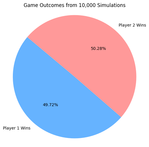
As , the distribution of the number of moves in a randomly played game, where all legal moves are equally likely, converges to a log-Gaussian distribution. Under these conditions, the game dynamics are sufficiently symmetric such that each player is equally likely to win.
This conjecture is supported by simulation data presented in Figure 2 and Figure 3, which suggest that the observed move counts exhibit the heavy-tailed, right-skewed characteristics consistent with a log-Gaussian distribution. Furthermore, the symmetry in the outcome frequencies aligns with the theoretical expectation of equal win probabilities for both players under a uniformly random move selection process.
4. Game Winning Strategy
Through exhaustive simulations, we investigated the existence of deterministic winning strategies for both players in the Two-Player Ordered Zeckendorf Game. Our computational experiments reveal that Player 1 possesses a winning strategy for all initial values up to . At , we observe the first instance where Player 2 can force a win under optimal play, indicating a potential transition point in the game’s strategic landscape. Interestingly, in all simulated games for , Player 2 is only able to force a win once, suggesting that Player 1 generally has a significant advantage, especially for smaller values of .
Due to the combinatorial explosion in the number of game states and legal move sequences, a full resolution of the winner for was computationally infeasible. The structure of the game tree grows rapidly with , and optimal strategies require deep lookahead and pruning heuristics that go beyond naive enumeration.
The existence of a general winning strategy for either player remains an open problem. Furthermore, due to the game’s nontrivial dynamics and the subtle impact of move orderings on future legal moves, it is possible that the game exhibits regions of alternating player advantage or chaotic behavior in terms of outcome predictability.
Future work could include developing a minimax-based heuristic search with alpha-beta pruning to more efficiently explore deeper game trees and extract structural insights into what governs winning positions. Additionally, identifying game invariants or monotonic features that correlate with winning states could pave the way toward a formal characterization of optimal strategies.
5. Conclusion
We have introduced and analyzed a novel ordered variant of the Zeckendorf game. We established key theoretical results, including termination guarantees, asymptotic bounds on the maximum number of moves, and lower bounds on the minimal number of required moves. Our study combines combinatorial structure with game dynamics, revealing rich mathematical behavior in even small initial configurations.
Despite our progress, many open questions remain.
-
•
Optimal Strategy Characterization: Can we rigorously prove the existence and form of an optimal winning strategy for Player 1 or Player 2 across all ? Is the observed dominance of Player 1 for small a universal phenomenon, or do other exceptions arise at larger scales?
-
•
Maximal Game Length Proof: While we conjecture a quadratic asymptotic growth and provide a priority-based strategy achieving near-maximal length, a formal proof of optimality remains open. Can analytic or combinatorial tools be developed to close this gap?
-
•
Generalizations to Other Recurrences: How does the introduction of order and switching moves affect games based on generalized Fibonacci sequences, such as -bonacci sequences or non-constant recurrences? Do analogous termination and length results hold?
-
•
Probabilistic Analysis of Random Play: Our empirical evidence suggests a log-Gaussian distribution of move counts under uniform random play. Can this distribution be derived rigorously? What are the deeper probabilistic and ergodic properties of the random dynamics?
-
•
Computational Complexity and Algorithmic Approaches: Given the rapid growth of the game tree, can efficient algorithms or heuristics be developed to determine winning positions for larger ? Are there polynomial-time methods to approximate optimal strategies or game lengths?
-
•
Structural Invariants and Monovariants: Are there additional invariants or monotonic quantities beyond those currently identified that govern the evolution of game states? How might these guide strategic reasoning or simplify analysis?
-
•
Multiplayer or Alliance Variants: Extending to more than two players or cooperative alliances—how do order and adjacency constraints reshape the strategic landscape? Can these variants be fully characterized or related to known combinatorial game theory frameworks?
These questions point toward deeper connections with additive number theory, algorithmic game theory, and dynamical systems. We believe this variant offers a promising platform for further exploration of combinatorial games and integer representations.
All simulations and visualizations used in our analysis were implemented in Python and C++, and the full codebase is publicly available at https://github.com/vraneskoy/zeckendorf_ordered_game.
6. Appendix
The following two figures provide computational evidence in support of Conjecture 3.2.
Corollary 1.12 gives us an error term in our upper bound on maximal game length of . The following figure provides an estimation for the constant before the term.
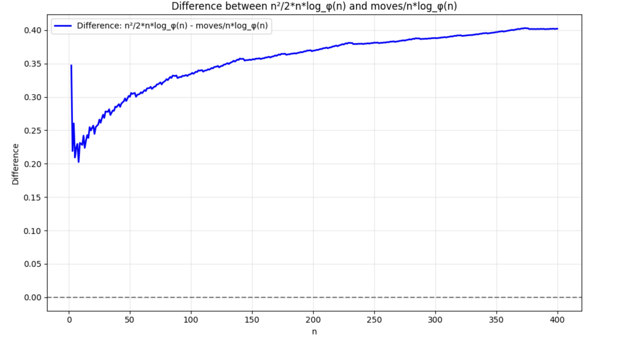
converges to a number bigger than 0.4 and much lower than 1.
References
- [1] Paul Baird-Smith, Alyssa Epstein, Kristen Flint, and Steven J Miller. The Zeckendorf Game. In Combinatorial and Additive Number Theory, New York Number Theory Seminar, pages 25–38. Springer, 2018.
- [2] Paul Baird-Smith, Alyssa Epstein, Kristen Flint, and Steven J Miller. The generalized Zeckendorf game. The Fibonacci Quarterly, 57(5):1–14, 2019.
- [3] Olivia Beckwith, Amanda Bower, Louis Gaudet, Rachel Insoft, Shiyu Li, Steven J Miller, and Philip Tosteson. The average gap distribution for generalized Zeckendorf decompositions. The Fibonacci Quarterly, 51(1):13–27, 2013.
- [4] Elżbieta Bołdyriew, Anna Cusenza, Linglong Dai, Pei Ding, Aidan Dunkelberg, John Haviland, Kate Huffman, Dianhui Ke, Daniel Kleber, Jason Kuretski, et al. Extending Zeckendorf’s theorem to a non-constant recurrence and the Zeckendorf Game on this non-constant recurrence relation. The Fibonacci Quarterly, 58(5):55–76, 2020.
- [5] Anna Cusenza, Aidan Dunkelberg, Kate Huffman, Dianhui Ke, Daniel Kleber, Steven J Miller, Clayton Mizgerd, Vashisth Tiwari, Jingkai Ye, and Xiaoyan Zheng. Winning strategy for multiplayer and multialliance Zeckendorf games. The Fibonacci Quarterly, 59(4):308–318, 2021.
- [6] Alexandre Gueganic, Granger Carty, Yujin H Kim, Steven J Miller, Alina Shubina, Shannon Sweitzer, Eric Winsor, and Jianing Yang. Limiting distributions in Generalized Zeckendorf Decompositions. The Fibonacci Quarterly, 57(2):109–125, 2019.
- [7] Murat Koloğlu, Gene S Kopp, Steven J Miller, and Yinghui Wang. On the number of summands in Zeckendorf decompositions. The Fibonacci Quarterly, 49(2):116–130, 2011.
- [8] Ruoci Li, Xiaonan Li, Steven J Miller, Clayton Mizgerd, Chenyang Sun, Dong Xia, and Zhyi Zhou. Deterministic zeckendorf games. The Fibonacci Quarterly, 58(5):152–160, 2020.
- [9] Édouard Zeckendorf. Representations des nombres naturels par une somme de nombres de fibonacci on de nombres de lucas. Bulletin de La Society Royale des Sciences de Liege, pages 179–182, 1972.