The peculiar velocity field up to by forward-modeling Cosmicflows-3 data
Abstract
A hierarchical Bayesian model is applied to the Cosmicflows-3 catalog of galaxy distances in order to derive the peculiar velocity field and distribution of matter within . The model assumes the CDM model within the linear regime and includes the fit of the galaxy distances together with the underlying density field. By forward modeling the data, the method is able to mitigate biases inherent to peculiar velocity analyses, such as the Homogeneous Malmquist bias or the log-normal distribution of peculiar velocities. The statistical uncertainty on the recovered velocity field is about 150 km/s depending on the location, and we study systematics coming from the selection function and calibration of distance indicators. The resulting velocity field and related density fields recover the cosmography of the Local Universe which is presented in an unprecedented volume of universe 10 times larger than previously reached. This methodology open the doors to reconstruction of initial conditions for larger and more accurate constrained cosmological simulations. This work is also preparatory to larger peculiar velocity datasets coming from Wallaby, TAIPAN or LSST.
keywords:
large-scale structure of Universe, dark matter, observations, galaxies: distances and redshifts, methods: data analysis1 Introduction
Peculiar motions of
galaxies are due to the gravitational interaction with the underlying
density field of matter. Thus peculiar velocities of galaxies are a
powerful and unbiased tool to study the dynamics and structure of the Local Universe.
Velocities have been used as probes of cosmological parameters (e.g. Zaroubi et al. (1997); Nusser &
Davis (2011); Feix
et al. (2017); Howlett
et al. (2017); Nusser (2017); Wang et al. (2018)), for
cosmography studies (Dekel
et al., 1999; Tully
et al., 2014; Courtois et al., 2017; Hoffman et al., 2017), and to
set initial conditions for constrained simulations (Gottloeber et al., 2010; Sorce
et al., 2016).
In the past, the Local Universe peculiar
velocity field has been reconstructed from the expected response to the observed redshift distribution of galaxies taken
as tracers of the mass distribution (Nusser &
Davis, 2011; Davis &
Scrimgeour, 2014; Hudson et al., 2004; Hong
et al., 2014; Scrimgeour
et al., 2016).
An alternate approach has been followed by the Cosmicflows program.
Peculiar velocities are inferred from departures of measured distances from the expectations of uniform cosmic expansion.
Cosmicflows catalogs (Tully et al., 2008; Tully
et al., 2013) have been analyzed
through the Wiener Filter/Constrained
Realizations methodology (WF/CR) (Zaroubi
et al., 1999; Courtois et al., 2012).
The assumption is made with the WF/CR methodology that
the measured velocities have a Gaussian noise and that their
2-point correlations are given by the CDM model.
It is critical that steps be taken to mitigate the Malmquist bias that arises from errors in distance. Objects are preferentially misplaced from regions of higher sampling density to lower sampling density (Strauss & Willick, 1995). As an example, it can be anticipated that galaxies assigned the greatest distances probably have large positive errors. These galaxies will be attributed with large negative peculiar velocities. The main objective of the present paper is to explore a more rigorous solution than the previous approach of Hoffman et al. (2015) in order to overcome this issue.
As a framework, Lavaux (2016) has developed a fully Bayesian algorithm that
incorporates the constrained realizations technique within a
statistical model accounting for the uncertainty on the location of
tracers. We use here a similar method to reconstruct the 3D linear
velocity field from Cosmicflows-3 data up to redshift .
The paper is organized as follows: the Cosmicflows-3 data is briefly described in Section 2 then the method is detailed in Section 3. The results includes an analysis on the reconstruction of the linear velocity field in Section 4 and an overlook on the resulting cosmography is given in Section 5. There are comments on outstanding issues in Section 6.
2 Data
2.1 Compilation of distance moduli
The reconstruction is based on the Cosmicflows-3 (CF3) catalog (Tully et al., 2016)111Available as a table at http://edd.ifa.hawaii.edu. CF3 provides a compilation of almost 18,000 galaxy distances, with the high redshift ones computed for the most part from three methodologies: the luminosity-linewidth relation of spiral galaxies, TF (Tully & Fisher, 1977), the Fundamental Plane of early-type galaxies (Djorgovski & Davis, 1987; Dressler et al., 1987), and Type Ia supernovae (Phillips, 1993). The absolute scale of the global distance ladder of these methodologies is given by galaxies that overlap with Cepheid variables (Leavitt & Pickering, 1912) or tip of the Red Giant Branch (Da Costa & Armandroff, 1990). The Surface Brightness Fluctuation (Tonry & Schneider, 1988) method helps providing a bridge between the near and far field. The CF3 compilation is heterogeneous, unlike concurrent single methodology samples (Springob et al., 2007; Springob et al., 2014; Hong et al., 2014). Indeed, when available, CF3 incorporates the major literature contributions. For inclusion in CF3, a source must usefully complement other components while overlapping sufficiently to assure consistency of scale. Each linkage has associated uncertainties. However, what is lost in the ambiguities of linkages is surely more than compensated by the dynamic range of the CF3 catalog. Nearby, coverage is dense and distances are accurate at the level of 5%. Farther away, Fundamental Plane contributions emphasize coverage of major clusters. TF samples preferentially provide distances to galaxies in the field. SNIa hosts are scattered serendipitously. The methodologies converge in groups where there can be multiple contributions. A group, or an individual galaxy where there is a convergence, has a unique distance. Averaged over all such cases, methodologies should agree.
2.2 Groups
Our goal is to derive the linear velocity field from the peculiar velocities of galaxies. However, galaxies in groups or clusters are affected by non linear motions which are not modeled within our CDM linear framework. Our solution is to average information over the small scale of groups. Tully (2015) provides a catalog of groups built from the 2MASS redshift survey complete to (Huchra et al., 2012). Candidate galaxies are either directly linked to these groups as members of the 2MASS sample or indirectly linked by close spatial and velocity association. A group is assigned a velocity that averages over all known members and a distance that is the weighted average over those constituents with the necessary measurements. Uncertainties with measures are reduced roughly as (depending on the details of the contributing methodologies), so groups are particularly high value entries in the CF3 catalog.
2.3 Selection function
Our Bayesian methodology (see Section 3) needs priors on the statistical distribution of distances. Because it is a composite catalog, CF3 is inhomogeneous both in distance and angular coverage. Consequently it does not admit a unique and simple selection function. Still, it is possible to identify 5 main subsamples based on the original observational surveys:
-
1.
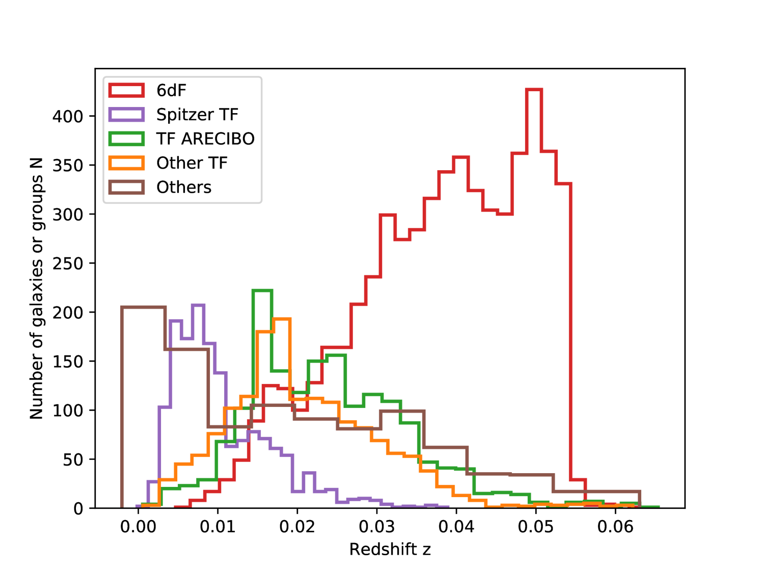
6dFGSv data provides the most well defined subsample: it has a high degree of completeness up to a sharp cutoff at . The subsample contains 5,777 galaxies or groups with a median redshift of .
-
2.
Another reasonably well defined subsample is based on the TF method with near-infrared photometry from Spitzer Space Telescope. This constituent gives particular emphasis to coverage at low galactic latitudes. The 1,546 galaxies or groups included in this subsample have a median redshift of .
-
3.
TF data is particularly deep within the region covered by Arecibo Telescope which observes galaxies of declination . The subsample contains 1,628 galaxies or groups with a median redshift of .
-
4.
Other TF data than in the Arecibo declination range. The subsample contains 1,569 galaxies or groups with a median redshift of .
-
5.
Other data coming from heterogeneous methodologies. Cepheids, tip of the red giant branch and surface brightness fluctuation contributions are local and of high accuracy. Groups which have more than ten members with known redshifts are included in this subsample. Group distances are mostly averaged over Fundamental Plane and TF measures with occasional SNIa contributions. Isolated SNIa lie over a wide range of redshifts up to . This last subsample does not have a simple selection function. This subsample contains 963 galaxies or groups with a median redshift of .
The total number of tracers in the catalog is . Figure 1 shows the redshift histograms of all these subsamples. We see that 6dF data plays a major role in CF3 and has a singular behavior with a sharp cutoff at redshift . Except for the last subsample of heterogeneous inputs, the other subsamples redshift distributions behave as expected: a growth at small distance due to the volume effect and then a decrease due to selection effects. We will show in Section 3.4.4 how we model these distributions.
3 Methodology
This section presents the methodology developed to reconstruct the linear velocity field underlying Cosmicflows-3 data.Our framework is assuming a CDM model and a Gaussian error model on the observations, the distance moduli and redshifts . As it will be described in the following sections, the parameter space includes the most probable luminosity distance of galaxies , an effective Hubble constant , a non-linear velocity dispersion and the linear velocity field itself v:
| (1) |
The general idea is to derive from basics assumptions the posterior probability of these parameters given the data and then sample from it. The sampling will result in the posterior distribution of the linear velocity field v from which we will extract the mean and standard deviation. The first subsection reminds the reader about the CDM model of peculiar velocity statistics while the next subsections will detail how the posterior probability is constructed and the procedure for sampling from this complex distribution.
3.1 Definitions and notations
The methodology relies on the assumption of a flat CDM model parametrized by the set of parameters . The CDM model assumes homogeneity and isotropy so that the cosmological redshift of a galaxy is related to its luminosity distance through the Hubble law:
| (2) |
where . Eq. 2 can be numerically inverted, giving . In the following we make the dependence implicit and note instead of . The analysis assumes the linear regime where the overdensity field is small . In this case the linear theory of perturbations predicts that the linear overdensity field is Gaussian and is described by its power spectrum :
| (3) |
where denotes the Fourier transform of and is the Dirac delta distribution. Gravitational dynamics in an expending universe dictates that the rotational component of the velocity decays early after the onset of the instability and to linear order the velocity v and density fields are related by:
| (4) |
where is the growth rate of structure and depends on the assumed cosmological parameters. Eq. 4 is linear as we can see by transposing it into the Fourier space:
| (5) |
Consequently, the statistic of v is also Gaussian. The statistic of v is described in the Appendix A.
Because of the peculiar velocity field v, the Hubble flow described in Eq. 2 is distorted, and the observed redshift of a galaxy is a composition of the cosmological redshift and the Doppler effect coming from the radial peculiar velocity:
| (6) |
where . The velocity field v can be divided into a linear and a non-linear part and the non-linear part is approximated here by an isotropic Gaussian probability distribution function:
| (7) |
where denotes the normal distribution of mean and variance over a variable and the conditional probability of given . From the measurements of galaxy distance moduli and redshifts , our goal is to infer the underlying peculiar velocity field v. Since the measurement of extragalactic distances is very noisy (most often about 20 of relative error), we must take into account the correlations between the observed redshifts to extract information on the velocity field. Also, we need to take into account the possible biases appearing when dealing with peculiar velocity field reconstruction, which is done in Section 3.2. The Section 3.4 present how to describe the observations given the above model.
3.2 Malmquist bias
Our model is motivated by a rigourous treatment of homogeneous and
inhomogeneous Malmquist bias. The homogeneous Malmquist bias
is a
statistical bias resulting
from a combination of the volume effect nearby and the selection effects
far away. The observational uncertainties on the measured
distances scatter the observed galaxies along the radial direction. Closeby, the number of galaxies grows with the distance, so that
overall it is more likely to underestimate the galaxy distances, and as
a consequence to assign erroneously positive peculiar velocities (Strauss &
Willick, 1995). At large
distances, the effect is the opposite:
it is more likely that the galaxies we observe are scattered away from
us, and so in average we overestimate their distances, and assign
erroneously negative peculiar velocities. Consequently, neglecting the
homogeneous Malmquist bias would create a fake
outflow in the central region and a fake inflow on the edges. To
overcome this bias, our statistical model fits the underlying most probable
luminosity distances of galaxies, together with the velocity
field. The bias is statistically handled by attributing a prior
function to these distances. The shape of the prior function will be
detailed in Section 3.4.4, and will be chosen so
that both the volume effect and selection effects are taken into
account.
The related inhomogeneous Malmquist bias arises from structure in the observed volume. In the vicinity of a dense region, galaxies are more likely to be scattered from denser to less dense regions. Consequently, the inferred peculiar velocities are biased toward a stronger inflow onto the structures, and thus bias the reconstructed velocity field. By introducing the luminosity distances as parameters, our method is able to reduce this bias. Distances are inferred by both the observations and the reconstructed velocity field, and at each step the galaxies are relocated with respect to the velocity field at their positions. Consequently, an inflow on a dense region will shift the distances toward their true positions. For a more complete analysis of the Malmquist bias, we refer the reader to Strauss & Willick (1995).
3.3 Observed radial peculiar velocities
The appropriate modeling of the distribution of errors on the observed peculiar velocities is an another important concern. The peculiar velocities are not directly measured but are usually derived from the distance moduli and redshifts measurements through the Eq. (6), where the luminosity distances are computed from the distance moduli using:
| (8) |
Since the errors on the distance moduli are supposed to be Gaussian, the resulting distribution of peculiar velocities will not be Gaussian distributed but rather Log-normal distributed (Tully et al., 2016). An example of treatment of this effect is given by Watkins & Feldman (2015) who suggest the use of an unbiased estimator of peculiar velocities with Gaussian distributed errors and which is valid at distances Mpc.
We use in this paper a different approach. Instead of analyzing the observed peculiar velocities, we rather choose to model the distance moduli observations directly. To do so, the introduction of the luminosity distances as free parameters allow us to take into account the Gaussian distribution of distance moduli errors including the relativistic effects of Eq. (6). The statistical linkage between distance moduli and luminosity distances will be explained in Section 3.4.1.
3.4 Statistical model
We aim at recovering the linear peculiar velocity field from the CF3 observations. We work in a Bayesian framework and try to estimate the posterior probability of v given the model described above and the observations. We proceed in three steps. First, we detail how the likelihood of our observations is constructed (Sections 3.4.1, 3.4.2, 3.4.3); second we impose priors on the fitted parameters that come from the CDM model presented in the above section (Section 3.4.4). Third, we sample from from the posterior probability (Section 3.5).
3.4.1 Distance moduli
Distance indicators used in CF3 are expressed as distance moduli rather than luminosity distances. The link between the two is given by Eq. (8). Our primary interest in this study concerns deviations from cosmic expansion which are determined independently of the absolute scaling of the extragalactic distance ladder. In addition, our analysis is insensitive to a potential monopole term that might reflect that we live in an overall under or overdense part of the universe. Tully et al. (2016) argued that the value of the Hubble Constant consistent with the 18,000 distances in CF3 is km s-1 Mpc-1 to within , discounting the irrelevant absolute scaling. There is agreement at this level in the determination of between the sample within and samples of SNIa at , limiting concern of a substantial local monopole to flows.
Our conclusion regarding the matter of the Hubble Constant is that the value is relatively well determined but uncertainties at the few percent level remain that are relevant for our analysis. For this reason, we introduce a dimensionless free parameter to model this uncertainty in the constant:
| (9) |
If the absolute scale is compatible with the assumed , then
should be unity.
Because the distance moduli are very noisy, we need to model the observations by assuming that the error is Gaussian (noted ) and choose to fit for the underlying true luminosity distance :
| (10) |
The parameter is correlated to the reconstructed velocity field and is prone to systematics coming from shifts between zero-point scales of different methodologies, non-linear effects, selection functions and possible external bulk flows. For this reason, one needs to take this parameter with caution and not as direct measure of . For the location of a galaxy in space, the angular position is measured essentially without error. Hence, from the distance and the angular position, we can compute the spatial position of a galaxy, which we denote r.
3.4.2 Redshifts
Eq. 6 gives the relation between the observed redshift and the cosmological redshift , which can be computed from the luminosity distance through Eq.2. From these equations, we can compute the radial peculiar velocity of a galaxy:
| (11) |
In CF3, the errors on individual redshifts are not provided, and we chose to assume that they are measured with a Gaussian error of km/s, the typical error for a spectroscopic redshift measurement.
To model the redshifts measurements, we introduce the
underlying linear velocity field
sampled on a
grid of size and volume . Since the sampled velocity field is
linear, we need to model the departure of the observed velocities from
the linearity. We do so by introducing a Gaussian dispersion
around the linear field which is to be evaluated.The introduction of a unique parameter
hence models the departure of the
overall velocity field from linearity and does not model high
dispersion inherent to non-linear environment such as clusters of
galaxies. For this reason the use of the grouped CF3 catalog is
mandatory. Applying this model on the non-grouped catalog would
underestimate the redshift errors and lead to unphysical results near
high density regions.
The probability of observing the redshift knowing the luminosity distance and the velocity field v is:
| (12) |
where is defined by Eq. 11. Note that is here a function of the parameter and the observation , and does not correspond to a peculiar velocity measurement. The probability distribution above describes the statistical link between the redshifts and the model’s parameters. In practice, the linear velocity v in Eq. (12) is computed on a finite-size grid . To evaluate it at any position (such as the position of a galaxy), we use trilinear interpolation between grid cells. We note from the error distribution of Eq. (12) that and are strongly correlated, the two dispersions being different by only the relativistic factor . As a consequence, an over (or under) estimation of will be transferred to a under (or over) estimation of , and our results will be insensitive to the choice of .
3.4.3 Likelihood
The likelihood gives the conditional probability of our observations, namely the observed redshifts and distance moduli , given the model and its parameters, namely the true luminosity distance , the linear velocity field sampled on a grid v, , and . Since the conditional probabilities on and are independent, the likelihood is given by the combination of Eqs. (10) and (12):
| (13) |
where the index denotes the galaxy or group.
The likelihood defined by
Eq. (13) is similar to the one in Lavaux (2016)
but simplified
because we do not aim to fit the power spectrum properties such as the
shape or the normalization. Another difference is that we directly sample
the velocity field rather than the overdensity field. We do so to avoid
the use of Fourier Transform to compute Eq. (4) and hence to
not be subject to periodic boundary conditions. Also, we use a trilinear interpolation to compute
the linear velocity field at any point in space, while Lavaux (2016) developed
a Fourier-Taylor algorithm to interpolate using only series of Fast
Fourier Transforms. We note that our way of proceeding does not enforce the curl-free properties of the linear
velocity field. We a posteriori check that the curl part
of the reconstructed field is negligible.
From the likelihood (13), we can estimate the probability of a given velocity field v (and associated parameters) from the measurements of distance moduli and redshifts. This probability is given by the Bayes theorem:
| (14) |
where denotes the prior on the parameter , . The velocity field reconstruction is then obtained by sampling v from this probability distribution. Before explaining how the sampling is done, we turn now our attention to the definitions of priors.
3.4.4 Priors
We assume uniform priors on and (see Tab. 1). Following the model described in Section 3.1, we take into account the correlations between the peculiar velocities by adopting the following prior for :
| (15) |
where is the power spectrum and has been defined in Eq. 3. The corresponding prior on the linear velocity field is:
| (16) |
where denoted cartesian components and
is the velocity-velocity correlation tensor and is defined in the Appendix A.
Because of the aforementioned Malmquist biases, the prior on the distances can play a significant role in the analysis. We use two types of empirical priors. The first one is a piecewise normal distribution defined by:
| (17) |
where are the shape parameters of the function.
The second one is a power-law with an exponential cutoff, as proposed by Lavaux (2016) :
| (18) |
The normalization factor is non-analytical and is computed numerically.
These two priors have the properties that we expect for distance priors: they are bell-shaped curves allowing an asymmetry and with an exponential cutoff at large distance. The shape parameters allow for some flexibility of these priors and determine the mean value, standard deviation and skewness of the distributions. Since we are not able to establish the selection function(s) of CF3, we use an empirical approach and choose to fit the shape parameters together with the other parameters of the current model. Leaving these parameters free allow to take into account the volume and selection effects while not imposing strong constraints on derived luminosity distances. In practice, we attribute the prior to distances of subsamples (ii), (iii) and (iv) described in Section 2.3, and to distances of the 6dF subsample. Distances of subsample (v) are given a uniform prior. We will see in Section 4 that they describe correctly the posterior distribution of distances and in Section 6.1 the effect of changing the prior functions. The model parameters are summarized in Table 1.
| Fixed parameters | Description | Number | Notes and priors |
| Number of galaxy and groups | 1 | ||
| Length of the box side | 1 | Mpc/ | |
| One dimensional size of the grid | 1 | ||
| Distance moduli | N | Normally distributed with standard deviation . | |
| Errors on distance moduli | N | ||
| Observed redshift | N | Normally distributed with standard deviation | |
| Error on the observed redshifts | 1 | km/s/ | |
| Free parameters | |||
| v | The linear velocity field sampled on a grid | CDM prior defined by Eq. 16 | |
| Luminosity distances | Empirical priors defined by Eqs. 17 and 18 and/or uniform, depending on the membership in the subsamples defined in Section 2.2. | ||
| Effective shift of the distance moduli scale | 1 | Uniform prior within | |
| Gaussian standard deviation modeling the departure from linearity | 1 | Uniform prior within km/s | |
| Hyperparameters defining the distance priors shapes | Uniform priors depending on the prior function |
3.5 Sampling
After we have constructed the likelihood and the priors of the model, we need to sample v from the posterior distribution given by Eq. (14). In this section, we briefly explain how this sampling is done by a Markov Chain Monte Carlo (MCMC) method. For more technical details, the reader is referred to Lavaux (2016). The sampling method is the partially collapsed blocked Gibbs sampling algorithm. Gibbs sampling is a MCMC method where each parameter is drawn from its conditional probability given the other parameters. Schematically, if we want to sample parameters , the sampling will be done using the following scheme down to the Markov step :
Our parameter space is:
| (19) |
and we need to compute each conditional probability from the likelihood. However, we note that is strongly correlated with the velocity field, and we draw this parameter from its conditional probability marginalized over the velocity field to make the sampling more efficient. This is called collapsed Gibbs sampling. At the end, our sampling is the following procedure:
-
1.
We first sample from the probability distribution marginalized over the velocity field:
(20) where is the vector of the galaxies radial peculiar velocities and C is the velocity autocorrelation matrix defined in the Appendix A. Those two quantities implicitly depend on the parameters and .
-
2.
We draw from the conditional probability:
(21) - 3.
-
4.
From the sampled constrained realization, we generate a new set of luminosity distances with the following probability:
(22) -
5.
Eventually we fit the hyperparameters of the distance prior functions over the generated distances.
This procedure is carried until convergence. At the end we have a number of realizations of all parameters following the posterior probability defined by Eq. (14). The reconstructed velocity field is assumed to be the mean of the linear velocity field samples and the error is the standard deviation. The method has been tested on different mocks by Lavaux (2016) and we test our specific implementation as described in Appendix C.
4 The Cosmicflows-3 peculiar velocity field
In this section we present the results of the method applied on CF3 catalog. We chose to assume . We fit the distance priors by the empirical function defined by Eq. 18 for the subsamples (ii,iii,iv) defined in Section 2.3. The distances from the subsample (i) corresponding to 6dF data are fitted assuming the function described by Eq. 17. We do so to ensure the possibility for the prior function to model a sharp cut-off in distances.
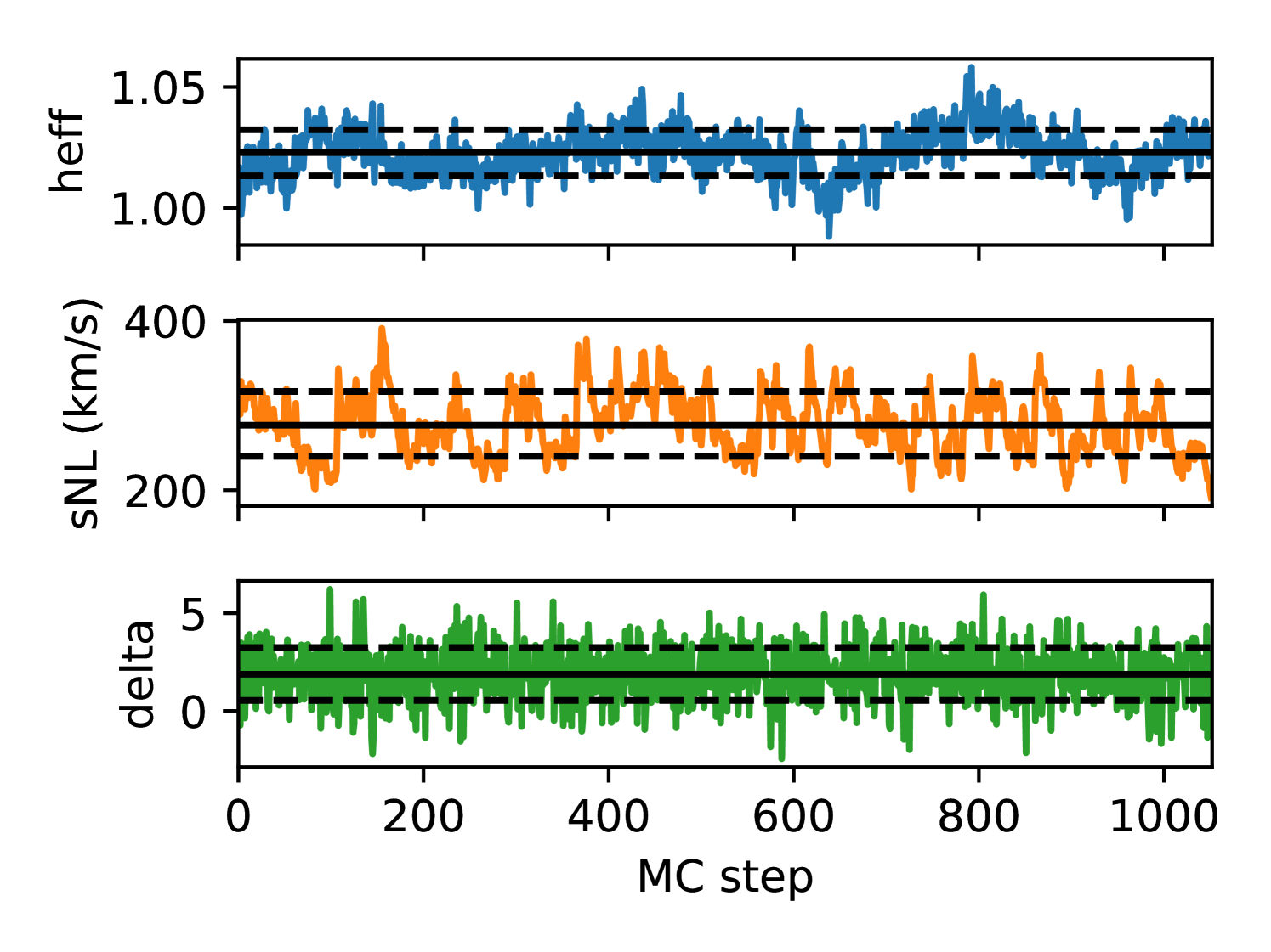

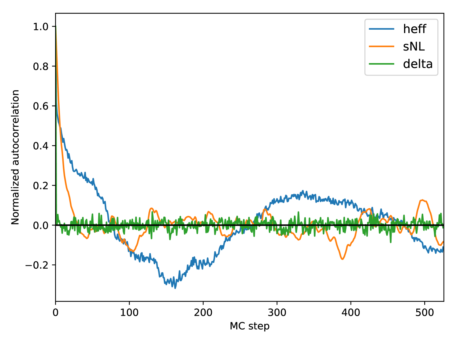
We fit for a global effective zero-point shift and assume the inter-calibration of distances determined by Tully et al. (2016) and the CMB frame transformations given by Tully et al. (2008). Figure 2 shows the resulting MCMC chain for the two parameters , and for the overdensity field reconstructed near the Virgo Cluster at location Mpc/ and the corresponding histograms are given in Fig. 3. We see from these two figures that the chain has globally converges and result in approximately Gaussian posterior distributions. To further evaluate the convergence of our Markov Chain, we plot in Fig. 4 the normalized autocorrelation of the chains for the two parameters and . The autocorrelation of a parameter for a correlation length is defined by:
| (23) |
where is the mean value of computed on the samples. The first decorrelation for a chain corresponds to the intersection with zero. We can see that the has a decorrelation length of about and the non-linear dispersion around steps. This suggests that over our 1400 MC steps, there is some 20 independent samples. For each parameter, the error on the mean of the distribution decreases, as after convergence and running the chain further will reduce this statistical error. We estimate here that the sampling error on the mean overdensity field (typically ) is sufficient considering the computation cost of the sampling.
We find , which suggests that the calibration of CF3 data is compatible with the assumed fiducial Hubble constant km/s/Mpc within . The non-linear dispersion parameter , which models our lack of knowledge about the non-linear part of the velocity field, is found at km/s. The fitted value of around 300 km/s appears to be high compared to the typical value of km/s. This can be due to underestimation of distance modulus errors, or redshifts errors which were set here at km/s for every galaxy. Also, this value depends on the efficiency of the grouping described Section 2.2 at removing entirely the non-linearities in groups of galaxies. Another possibility is that the trilinear interpolation used to compute the reconstructed radial velocity at the position of each galaxy artificially increases the departure from linearity modeled by . Overall this parameter absorbs uncertainties of our model.
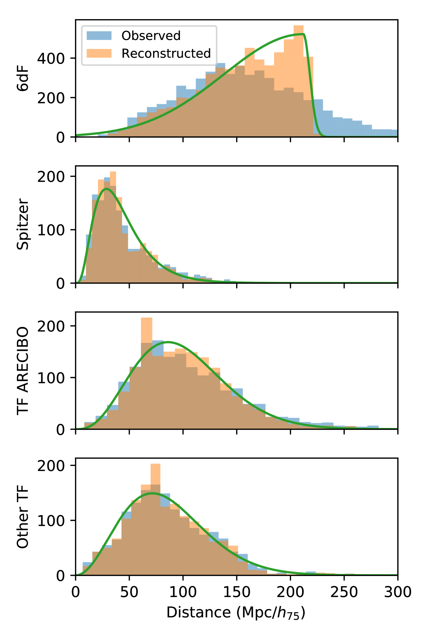
Figure 5 shows the fitted priors on the distances. Overall the shape of the priors is in agreement with the underlying distance distribution. The case of 6dF data might look surprising because there is a discrepancy between the fitted distances and the original ones. However, by considering the distribution in redshifts shown in Figure 1, we can see that the tail of the measured distance distribution is only due to observational errors and results from the convolution of the real distance distribution with the Gaussian of errors. This particular case illustrates the importance of imposing priors to model selection effects.
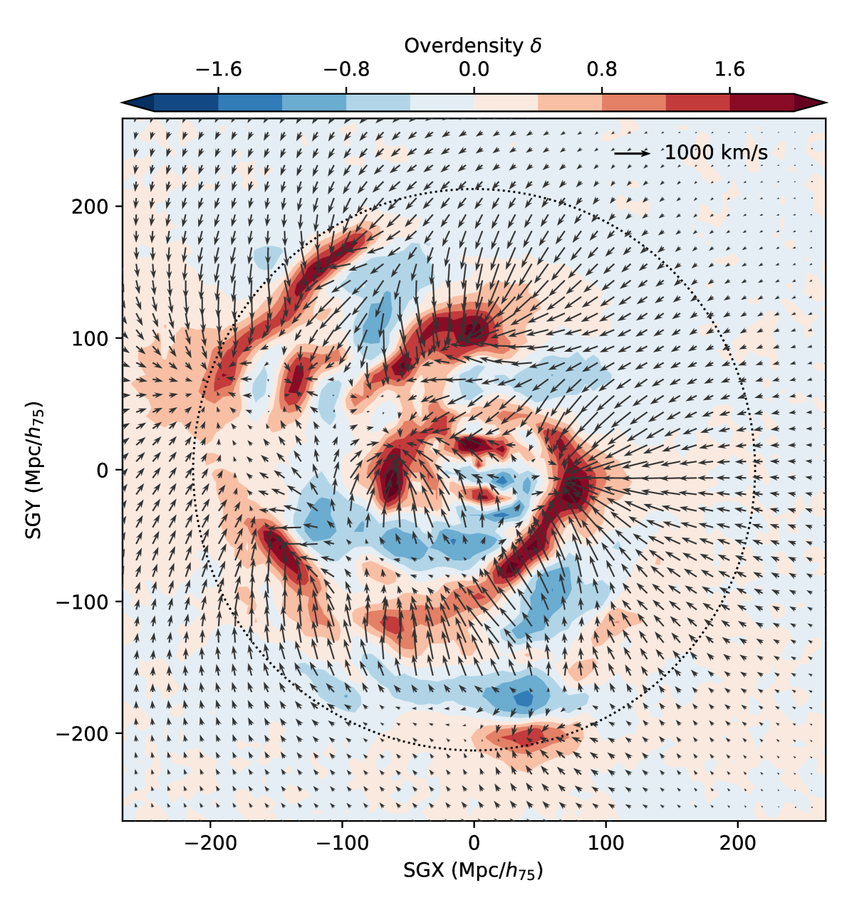
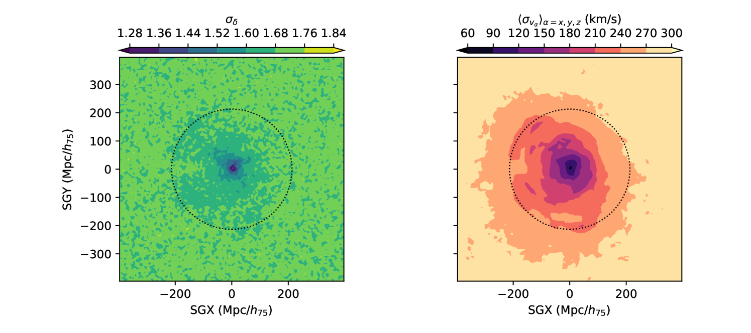
Eventually, the Mpc/ slice of the reconstruction is shown Figure 6. In this figure, the colormap corresponds to the reconstructed overdensity field and the black arrows to the tridimensional linear velocity field. We stress that the reconstructed overdensity and velocity fields are not computed one from another using Eq. 5, but rather sampled simultaneously222For each MC step, we draw both a constrained realization of the velocity field and overdensity field from a common random realization with Eqs. 35 and 37. The original field was computed in a box of width 800 Mpc/, and we show here the central 500 Mpc/ where the signal over noise is non-zero. We can see that the overdensity goes toward zero near the edges, because there are no observed galaxies at large distances. By eye, we can identify several cosmic structures that we will shortly list in Section 5. We also qualitatively see the match between the overdense structures and the velocity infalls. These fields come with statistical errors that can be computed from the resulting Markov Chain. The standard deviation of the reconstructed fields and are plotted in Fig. 7. At large distance, we recover the CDM standard deviation of the overdensity and velocity field. In particular, we recover the value of 300 km/s deviation for the velocity field. This is due to the absence of data points beyond , a limit which is illustrated by the black circle. We can see that the radial peculiar velocity field seems less noisy than the overdensity field. The reason is that the velocity field is more correlated than the overdensity as can be seen with Eq. 27. Consequently, the root mean square value of the posterior distribution does not capture entirely the correlated errors of the velocity field, and these errors correlate on larger scales. In the next section, we study the reconstructed overdensity field shown in the left panel of Fig. 6 and compare it with the actual distribution of galaxies to check the consistency with other observables.
5 Cosmography overview
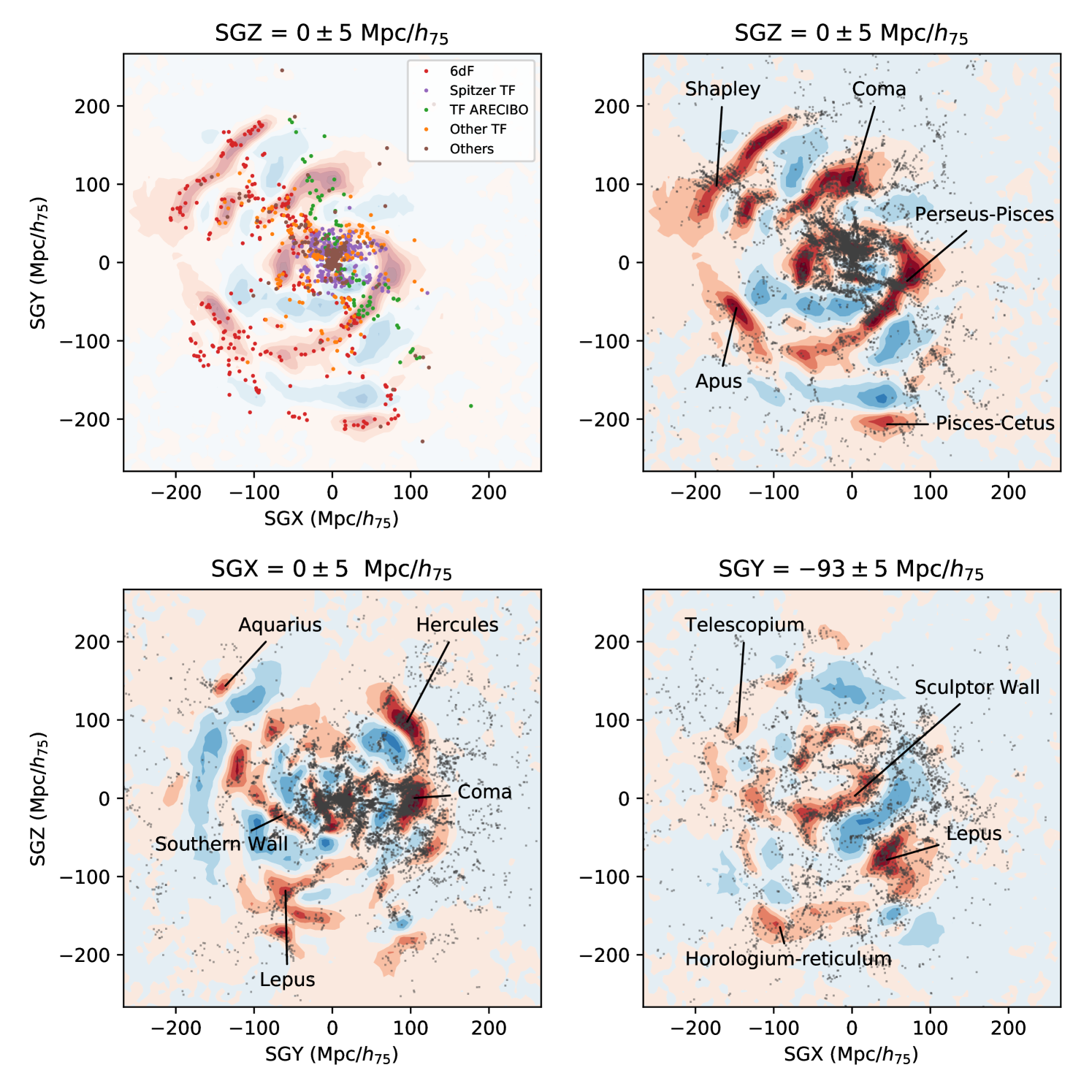
In this section we show partial results on the reconstructed overdensity field. A full description will be made in an upcoming cosmography paper. Main results are presented in Figure 8 where we plot the overdensity field in three different slices corresponding to coordinates Mpc/ (twice), Mpc/ and Mpc/ going from top left to bottom right. We first look at the two top panels. On the left, the colored dots represent CF3 data within a slab of 10 Mpc/ thickness, while on the right the dark dots are all available galaxies of the LEDA database located at their redshift positions within the same depth. The colored galaxies show the anisotropy of CF3 catalog. The southern hemisphere is mainly covered by 6dF galaxies (in red), while there are fewer data points in the northern hemisphere. Looking at the right panel, we can observe a good agreement between the reconstructed overdensity field and the location of galaxies. At large distances, we notice small discrepancies (for example around Mpc/ (top right panel)). The reconstructed structures seem to be shifted compared to the redshift positions. This issue is tightly linked to the recovered value of , which is prone to systematics. This might be a hint of a shift between zero-point calibrations depending on the region covered. We discuss this issue in Section 6.1. We add to the plots the name of some known structures, such as Coma, Shapley, Perseus-Pisces, Apus and Pisces-Cetus. The two bottom panels correspond to other slices of the Local Universe reconstruction. Again, there is agreement between the reconstructed overdense regions and the galaxy distribution. The bottom right panel exhibits some distant structures which are less known, such as the Southern Wall, Telescopium or Lepus.
6 Discussion
In this paper, we described our linear peculiar velocity field reconstruction method. We then applied it to the CF3 catalog, considering generic modeling of the prior distance distributions and potential shift on the zero-point calibration of all distances. We saw in Section 5 how this reconstruction can be used to study our local environment and the unbiased distribution of dark matter in the CDM framework. We now turn to the discussion of the limits and possible improvements of the presented method.
6.1 The Hubble Constant
We introduced an effective reduced Hubble constant to absorb uncertainty on the calibration of the distance indicators and assumed a Hubble constant of km/s/Mpc. It is worth noticing that the value of the effective Hubble constant is correlated with our choice of distance priors. This systematic is studied in Appendix D on a subsample of the CF3 catalog. We find that imposing uniform priors on the distances lowers the value of by around (equivalent of around 3 km/s/Mpc). This suggests that the parameter not only absorb uncertainties on the assumed Hubble Constant, but also compensate for residual homogeneous Malmquist bias that is not modeled by the simple shape of our distance priors.
The CF3 catalog contains distances from six distinct methodologies. With each of these methodologies there are contributions from multiple sources. It is fundamentally important that the distances from the diverse inputs be consistent in zero point and free of systematics with redshift. An important feature in the construction of CF3 was large overlaps between sources. The complex interlacing is discussed by Tully et al. (2016). The grounding assumption was all measurements of the distance to a galaxy or a cluster of galaxies should give the same value on average. The scale is bootstrapped from fundamental Cepheid and RR Lyrae calibrators in our galaxy. Consequently the CF3 product is distances in Mpc derived independently from knowledge of velocities.
There is one relatively weak link. The 6dF sample is a major component of CF3 that explores a domain that is poorly covered by other samples. The scale linkage is established through 84 individual galaxies with alternate measures and 381 groups with distances to members from alternate methods. Given the importance of the 6dF contribution, in Appendix E we consider the possibility of a scale mismatch by introducing an independent parameter associated with the 6dF contribution. A small difference is found between the optimal values for the 6dF component and the rest of the CF3 contributions, namely the effective Hubble constant is reduced by 3% for the 6DF sample. We find that the reconstructed radial velocity field is affected by the introduction of this additional parameter, and that the non-linear dispersion parameter is reduced by 20%. It is not clear, though, that the addition of a parameter has improved the model. The additional parameter for the 6dF component could mask velocity streaming specific to the sector uniquely sampled by 6dF. Our primary interest is to map the velocity field so for that purpose the conservative assumption is to not add an additional parameter. Rather, we assume that the 6dF distances were properly linked to the other CF3 components, and model departures from the fiducial are described by a single value of .
6.2 Non-linearities
The modeling of non-linearities can also be a source of systematics of our reconstruction. Our treatment involves the grouping described in Section 2.2. The merging of data within groups has clear advantages. While what we directly observe are individual galaxies, the test particles we want to follow in a linear reconstruction are collapsed haloes. If a halo contains multiple galaxies then we do best to average over the constituent properties. The groups are formulated from a large redshift catalog (Tully, 2015) and we average over the redshifts of all associated members. Then we find weighted averages of the distances from those group members in CF3. Distances of groups with many contributions can have low formal errors.
The remaining non linearities (outside of the groups) at redshift zero are modeled by a unique Gaussian dispersion to the observed velocities. The width of this distribution, namely , is fitted with the other parameters. This is an approximation: non-linear motions are correlated down to Mpc-1 scale and so are not randomly independent. However, including non-linear correlations within the actual method is a technical challenge since the correlations in the non-linear regime are not isotropic anymore. An interesting alternative is proposed by Hoffman et al. (2018) who try to use constrained simulations in order to reconstruct the non-linear part of the peculiar velocity field. Other options could also be tried like fixing the parameter at a value constrained by CDM non-linear simulation, or adding a discrete parameter for each galaxies to model their association to non-linear regions, such as in Lavaux (2016). The advantage of the latter method is to model both non-linearities and possible outliers.
6.3 Selection effects
Selection effects on distances play a considerable role in peculiar velocity analyses even though less critical than in galaxy number counts analysis. We described in Section 3.2 the Malmquist biases appearing when the selection effects are not properly modeled. In our Bayesian approach, the selection effects are modeled by constructing the probability of a galaxy having a luminosity distance knowing that we observed it. Our model suppose that this probability only depends on the actual distance and fitted hyperparameters (, , ). In particular, individual CF3 distances are unbiased (Tully et al., 2016), and the probability does not depend on the observed distance modulus .
We note however that selection effects would need further investigation in future works on peculiar velocities. As suggested by Hinton et al. (2017), a proper model needs the introduction of the generalized likelihood :
| (24) |
where the integration is over all possible observational data . Since the selection function of CF3 is not analytical it is challenging to write the term representing the probability of selecting a galaxy measurement given its overall properties and the model’s free parameters. Sampling from the extended likelihood is consequently hard and unpractical for the current analysis.
Our approach, while it is approximate, is robust and secure since we fit the priors directly on the reconstructed distances. Doing so, we value CF3 distances over eventual prior information. Also, it is worth noticing that the CF3 catalog benefits from the multiplicity of methods included in it. The selection effects being different from one methodology to another, the overall reconstructed velocity field should not be subject to individual method specificity. As mentionned in Section 6.1, we tested the effect of changing the priors on the distances and the results are presented in Appendix D.
7 Conclusions
This article presents an algorithm to reconstruct the linear peculiar velocity field up to from the Cosmicflows-3 catalog. We have been able to reconstruct for the first time the Local Universe velocity field from Cosmicflows-3 data, and showed some results in terms of cosmography. We also associated a corresponding map of statistical errors on both the overdensity and velocity field. The reconstructed field will be used for both cosmological analysis and cosmography. We have stressed the limits of the current method, especially about the model of non-linearities and selection effects. We showed that these effects were not completely negligible and should be more precisely modeled in future analyses.
Above all, this article highlights the ability of peculiar velocities to probe the matter distribution. With only about 11,000 tracers, we were able to map and identify overdense and underdense regions in the Local Universe, and showed the good agreement with redshift surveys containing more than 150,000 galaxies. As suggested by Lavaux (2016), the model could be extended to estimate cosmological parameters such as the Hubble constant or the growth rate . With upcoming large distance datasets, coming from TAIPAN (da Cunha et al. (2017), FP distances), WALLABY (Duffy et al. (2012), TF distances) and LSST (Lochner et al. (2018), SNIa distances), peculiar velocity analyses will need an accurate model to avoid systematics in the determination of cosmological parameters. The method presented here is to be considered as a baseline of such model.
Acknowledgements
R.G. thanks Mickael Rigault for fruitful discussions. We are grateful to the colleagues maintaining LEDA Lyon extragalactic database Dmitry Makarov and Philippe Prugniel. This research was supported by Institut Universitaire de France and CNES. This project has received funding from the European Research Council (ERC) under the European Union’s Horizon 2020 research and innovation programme (grant agreement No 759194 - USNAC).
References
- Courtois et al. (2012) Courtois H. M., Hoffman Y., Tully R. B., Gottlöber S., 2012, ApJ, 744, 43
- Courtois et al. (2017) Courtois H. M., Tully R. B., Hoffman Y., Pomarede D., Graziani R., Dupuy A., 2017, preprint, (arXiv:1708.07547)
- Da Costa & Armandroff (1990) Da Costa G. S., Armandroff T. E., 1990, AJ, 100, 162
- Davis & Scrimgeour (2014) Davis T. M., Scrimgeour M. I., 2014, MNRAS, 442, 1117
- Dekel et al. (1999) Dekel A., Eldar A., Kolatt T., Yahil A., Willick J. A., Faber S. M., Courteau S., Burstein D., 1999, ApJ, 522, 1
- Djorgovski & Davis (1987) Djorgovski S., Davis M., 1987, ApJ, 313, 59
- Dressler et al. (1987) Dressler A., Lynden-Bell D., Burstein D., Davies R. L., Faber S. M., Terlevich R., Wegner G., 1987, ApJ, 313, 42
- Duffy et al. (2012) Duffy A. R., Meyer M. J., Staveley-Smith L., Bernyk M., Croton D. J., Koribalski B. S., Gerstmann D., Westerlund S., 2012, MNRAS, 426, 3385
- Feix et al. (2017) Feix M., Branchini E., Nusser A., 2017, MNRAS, 468, 1420
- Gorski et al. (1989) Gorski K. M., Davis M., Strauss M. A., White S. D. M., Yahil A., 1989, ApJ, 344, 1
- Gottloeber et al. (2010) Gottloeber S., Hoffman Y., Yepes G., 2010, preprint, (arXiv:1005.2687)
- Hinton et al. (2017) Hinton S. R., Kim A., Davis T. M., 2017, preprint, (arXiv:1706.03856)
- Hoffman & Ribak (1991) Hoffman Y., Ribak E., 1991, ApJ, 380, L5
- Hoffman et al. (2015) Hoffman Y., Courtois H. M., Tully R. B., 2015, MNRAS, 449, 4494
- Hoffman et al. (2017) Hoffman Y., Pomarède D., Tully R. B., Courtois H. M., 2017, Nature Astronomy, 1, 0036
- Hoffman et al. (2018) Hoffman Y., et al., 2018, Nature Astronomy,
- Hong et al. (2014) Hong T., et al., 2014, MNRAS, 445, 402
- Howlett et al. (2017) Howlett C., et al., 2017, MNRAS, 471, 3135
- Huchra et al. (2012) Huchra J. P., et al., 2012, ApJS, 199, 26
- Hudson et al. (2004) Hudson M. J., Smith R. J., Lucey J. R., Branchini E., 2004, MNRAS, 352, 61
- Lavaux (2016) Lavaux G., 2016, MNRAS, 457, 172
- Leavitt & Pickering (1912) Leavitt H. S., Pickering E. C., 1912, Harvard College Observatory Circular, 173, 1
- Lochner et al. (2018) Lochner M., et al., 2018, arXiv e-prints, p. arXiv:1812.00515
- Nusser (2017) Nusser A., 2017, MNRAS, 470, 445
- Nusser & Davis (2011) Nusser A., Davis M., 2011, ApJ, 736, 93
- Phillips (1993) Phillips M. M., 1993, ApJ, 413, L105
- Planck Collaboration et al. (2015) Planck Collaboration et al., 2015, preprint, (arXiv:1502.01589)
- Scrimgeour et al. (2016) Scrimgeour M. I., et al., 2016, MNRAS, 455, 386
- Sorce et al. (2016) Sorce J. G., et al., 2016, MNRAS, 455, 2078
- Springob et al. (2007) Springob C. M., Masters K. L., Haynes M. P., Giovanelli R., Marinoni C., 2007, ApJS, 172, 599
- Springob et al. (2014) Springob C. M., et al., 2014, MNRAS, 445, 2677
- Strauss & Willick (1995) Strauss M. A., Willick J. A., 1995, Phys. Rep., 261, 271
- Tonry & Schneider (1988) Tonry J., Schneider D. P., 1988, AJ, 96, 807
- Tully (2015) Tully R. B., 2015, AJ, 149, 171
- Tully & Fisher (1977) Tully R. B., Fisher J. R., 1977, A&A, 54, 661
- Tully et al. (2008) Tully R. B., Shaya E. J., Karachentsev I. D., Courtois H. M., Kocevski D. D., Rizzi L., Peel A., 2008, ApJ, 676, 184
- Tully et al. (2013) Tully R. B., et al., 2013, AJ, 146, 86
- Tully et al. (2014) Tully R. B., Courtois H., Hoffman Y., Pomarède D., 2014, Nature, 513, 71
- Tully et al. (2016) Tully R. B., Courtois H. M., Sorce J. G., 2016, AJ, 152, 50
- Wang et al. (2018) Wang Y., Rooney C., Feldman H. A., Watkins R., 2018, MNRAS, 480, 5332
- Watkins & Feldman (2015) Watkins R., Feldman H. A., 2015, MNRAS, 450, 1868
- Zaroubi et al. (1997) Zaroubi S., Zehavi I., Dekel A., Hoffman Y., Kolatt T., 1997, ApJ, 486, 21
- Zaroubi et al. (1999) Zaroubi S., Hoffman Y., Dekel A., 1999, ApJ, 520, 413
- da Cunha et al. (2017) da Cunha E., et al., 2017, Publ. Astron. Soc. Australia, 34, e047
Appendix A Linear peculiar velocity distribution in the CDM model
Our framework is the linear theory of structure formation within a flat CDM model. The initial perturbations of such Universe are characterized by their Gaussian statistics as observed from the Cosmic Microwave Background (Planck Collaboration et al., 2015). In the linear theory, the Fourier modes of these perturbations has grown independently and the overdensity field of our Local Universe can still be described by its power spectrum :
| (25) |
where is the Fourier transform of . Such a linear approximation is only valid at large scales, i.e. , and consequently the present analysis aims at recovering only the very large scale structures, down to scales of few tens of Mpc. Given the cosmological growth rate ( depends on the adopted cosmology), one can compute the velocity field by:
| (26) |
which can be written in Fourier space as:
| (27) |
Consequently, the velocity-velocity two point correlation tensor is, in configuration space:
| (28) |
In practice, can be expressed using the radial and transverse correlations functions and (Gorski et al., 1989):
| (29) |
| (30) |
| (31) |
where and are the zero and first order spherical Bessel functions and is the Kroenecker delta. In practice, we use tabulated and , and use linear interpolation between the sampled positions. We also define the covariance matrix C of a set of radial peculiar velocities by:
| (32) |
Usually, the matrix of errors is taken as the sum of the error on the redshift measurement plus a dispersion due to non-linearities at , :
| (33) |
Appendix B The Hoffman-Ribak algorithm
The marginalized probability density for the overdensity field is
| (34) |
To sample from this probability density function Hoffman & Ribak (1991) proposes the following. From the power spectrum is generated a random realization . Then, a constrained realization is computed with the previous random part and a correlated one:
| (35) |
where is a constraint on the sampled field, here the radial peculiar velocities . The matrix is defined in Appendix A, and the correlation between the overdensity field and the radial peculiar velocity is:
| (36) |
It is also possible to directly sample the velocity field using :
| (37) |
where the index corresponds to the cartesian component. The correlation is given by
| (38) |
In this paper, we sample both the velocity and density field using the same random realization. We thus don’t need the periodic boundary conditions implied by the use of fast Fourier transform to evaluate Eq. 4.
Appendix C Test on mock
We test the implementation of the algorithm on a mock catalog of 4000 tracers generated as follow :
-
•
The angular positions are drawn from an uniform distribution,
-
•
The distances are drawn from a truncated normal distribution within Mpc,
-
•
We mimic the observations by computing the corresponding distance moduli and scatter them following a normal distribution of standard deviation ,
-
•
We input a shift in the distance moduli scale of .
-
•
From a random realization generated from a power spectrum truncated at 0.1 Mpc (to avoid non-linearities), we draw the peculiar velocities. We add a non-linear dispersion with km/s,
-
•
From the original distances and peculiar velocities, we compute the measured redshifts and add a Gaussian dispersion of km/s,
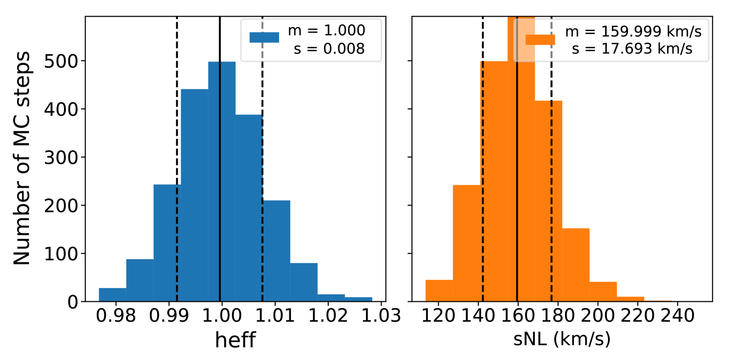
From the simulated distance moduli and redshifts, we reconstruct the velocity field following the procedure described in Section 3.5. We compute it on a grid of size and box of Mpc width. The Figure 9 shows the resulting distribution for the two parameters and , which both agree with their fiducial values.
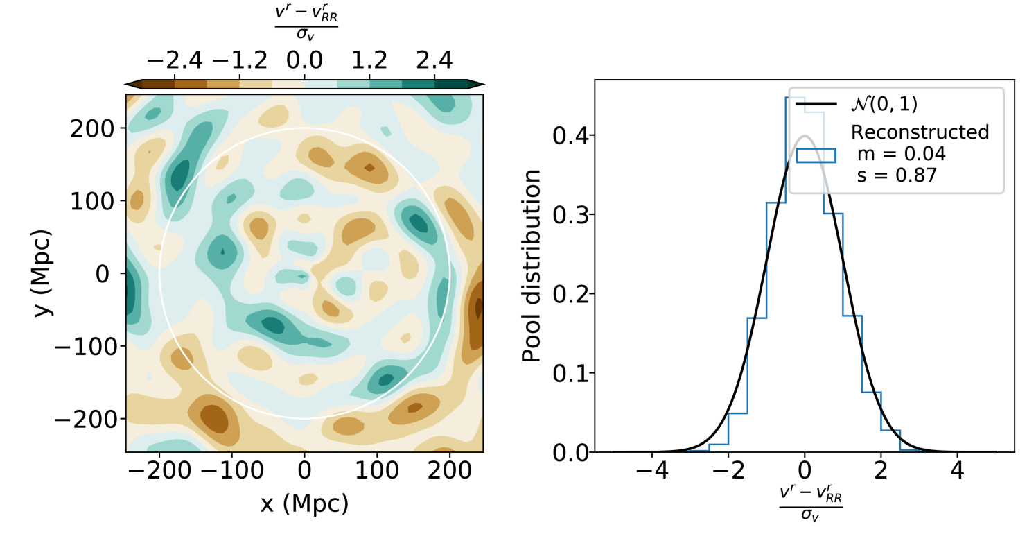
The comparison between the original Gaussian random field and the reconstructed radial velocity field is shown on Figure 10. The left panel shows the pull distribution of the reconstructed radial velocity field in the slice. On the left plot, we show the histogram of these values within the white circle corresponding to the data limit. Overall the distribution is close to a unit Gaussian, showing the unbiased aspect of the reconstruction. Also, on the left panel, there is no clear sign of reconstructed structures over more than .
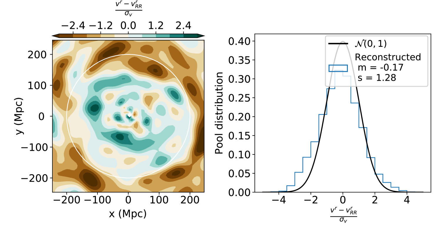
For comparison, the same plot is done using the WF/CR technique alone, i.e fixing the parameters , and , is shown on Figure 11. We can see the strong improvement from the method. Homogeneous Malmquist bias affects the distances so that there is excessive outflow in the center of the box and inflow outside, as it is described in Section 3.2.
Appendix D Changing the distance priors
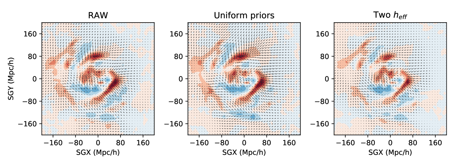
We test the effect of changing the assumed priors on distances on a subsample of the CF3 catalog. The test catalog is built by randomly taking half of the galaxies in each subsample defined in Section 2.3. The reconstruction is done on a grid of size . The reconstruction was carried in the case of uniform priors imposed on all distances except the 6dF one. We treat 6dF as separate because the sharp cutoff on their redshift makes the analysis unrealistic with uniform prior. On 6dF, we fit an empirical prior defined by Eq. 18. The calculation was carried on 800 MCMC steps and the first 300 are considered as the warmup phase. The Figure 12 shows the resulting histograms for the and parameters. One can see that the effective Hubble constant has been minored compared to the reconstruction shown in Figure 3 by more than one sigma. This shows the strong dependance of any Hubble constant determination with this method on the prior distance distributions. Figure 13 shows the comparison between the reconstructed fields in the case of a nominal reconstruction (empirical priors and unique shift in the zero-point) (left) and the case of uniform priors (middle). The differences are small, but one can notice the inflow on the Mpc/ part (data which is mainly not covered by 6dF data) has been increased. Because we imposed no priors on the data, the distances are more likely to be overestimated far away, and consequently the radial velocities underestimated, biasing the field towards negative values. This results shows that the prior distribution has an impact in our Bayesian analysis and underlines the fact that selection effects have to be properly modeled to extract cosmological parameters from the velocity field reconstruction.

Appendix E Considering 6dF as a separate subsample
We try to fit two different reduced effective Hubble constants , one for 6dF data and the other for the rest of the data. The distance priors are kept to empirical prior functions defined by Eq. 18. The resulting histograms are shown on Figure 14. We see that the values recovered for the two parameters are different while still compatible. We can see that the non-linear dispersion has decreased compared to the main and uniform priors reconstructions ( km/s compared to km/s). This suggests a better fit of the underlying velocity field. However, it could also be due to the artificial reduction of a real flow between 6dF covered region and the rest, which is why the main result of this article assumes a unique zero-point shift. Again, Figure 13 shows the comparison between the reconstructed fields in the case of a fiducial reconstruction (empirical priors and unique shift in the zero-point) (left) and the case of two different (right). The differences are more pronounced: The inflows in the regions Mpc/ and Mpc/ have been reduced. Also, we can see from the overdensity field that the overall inflows on structures have changed between the left and right panels, increasing in the case of a unique zero-point. We stress that the difference of flows can be artificial and the conservative approach taken in the main result of this paper (empirical priors and unique zero-point shift) should be preferred. However, this test shows that small shifts in distance indicators calibrations change the mean inflow on structures, and could have an impact on the determination of cosmological parameters, such as the growth rate or the Hubble constant . This impact is however beyond the work presented in this paper. Extending the model to the determination of cosmological papers from peculiar velocities is to be considered as a possible development of the current methodology.
