The Power Spectrum of Turbulence in NGC 1333: Outflows or Large-Scale Driving?

The structure of density and velocity fields in giant molecular clouds can be characterized by extended power laws (e.g. Heyer and Brunt 2004; Padoan et al. 2004, 2006), with scaling exponents consistent with those of numerical simulations of supersonic turbulence (e.g. Padoan et al. 2007; Kritsuk et al. 2007, 2009a,b). The existence of these scaling laws and of one-point statistics of turbulent flows (for example the probability distribution of gas density) is an important assumption in statistical theories of star formation aimed at the prediction of the stellar initial mass function (Padoan and Nordlund 2002, 2004; Hannebelle and Chabrier 2008, 2009) and the star formation rate (Krumholz and McKee 2005; Padoan and Nordlund 2009).

Is this assumption of a universal large-scale turbulent cascade valid in cluster-forming regions, believed to be the birthplace of most stars, or is the turbulence there driven internally by stellar outflows? As an alternative to the idea that stellar clusters are formed in one crossing time (Elmegreen 2000), Tan, Krumholz, and McKee (2006) propose that stars are formed in protocluster clumps over several dynamical times, while the turbulence is driven by stellar outflows. This scenario is investigated analytically by Matzner (2007) and numerically by Nakamura and Li (2007), Carroll et al. (2007), and Wang et al. (2009).

Nakamura and Li (2007) find that the velocity power spectrum in their outflow-driven simulation is very shallow above a characteristic scale of energy injection by outflows, $\ell_{\rm{inj}}$. They derive $\ell_{\rm inj}\approx 0.3$ pc, assuming their computational domain has a size $L=1.5$ pc and a total mass $m_{\rm tot}=929$ m_⊙, characteristic of cluster-forming regions. This value of $\ell_{\rm inj}$ and the flattening of the power spectrum at larger scales is consistent with the analytical results in Matzner (2007). Carroll et al. (2009) confirm the results of Nakamura and Li (2007) at higher numerical resolution, producing velocity power spectra even more clearly peaked at the outflow driving scale. With the values of mass, column density, and outflow momentum per unit mass, $v_{\rm c}=50$ km/s, adopted by Nakamura and Li (2007), equation (38) in Matzner (2007) gives $\ell_{\rm inj}=0.27$ pc. The injection scale is only weakly dependent on $v_{\rm c}$, $m_{\rm tot}$, and the star formation rate, and is approximately given by $\ell_{\rm inj}\approx 0.079\,\Sigma_{\rm cgs}^{-15/28}$ pc, where $\Sigma_{\rm cgs}$ is the column density in g/cm². Our conclusions do not critically depend on a precise knowledge of $\ell_{\rm inj}$, as long as scales just above $\ell_{\rm inj}$ are resolved in the observations.

The prototype of outflow-driven cluster-forming regions chosen by Nakamura and Li (2007), Matzner (2007), and Carroll et al. (2009) is NGC 1333 in Perseus. In this Letter, we derive the power spectrum of integrated intensity, $P_{I}(k)$, and velocity, $P_{v}(k)$, in NGC 1333, based on the data from the Five College Radio Astronomy Observatory (FCRAO) survey of the Perseus molecular cloud complex (Ridge et al. 2006), publicly available from the COMPLETE website. We show that the scale $\ell_{\rm inj}$ is resolved by the observations, and both power spectra, $P_{I}(k)$ and $P_{v}(k)$, are consistent with power laws extending to large scale, with the same slope found in supersonic turbulence simulations and in the Perseus complex on larger scale (Padoan et al. 2006). The constant slopes of $P_{v}(k)$ and $P_{I}(k)$ above the scale $\ell_{\rm inj}$ suggest that outflows may not be the dominant driving mechanism. In a recent paper appeared after the submission of this Letter, Brunt, Heyer, and Mac Low (2009) have reached the same conclusion for NGC 1333 and for other molecular cloud regions using a different method.

We first confirm the validity of the velocity coordinate spectrum (VCS) method of Lazarian and Pogosyan (2006), using synthetic maps of the $J$=1-0 line of ¹³CO, computed with a non-LTE radiative transfer code (Juvela and Padoan 2005), based on the density and velocity fields from a snapshot of a simulation of supersonic hydrodynamic turbulence with rms Mach number $\mathcal{M}$=6. These synthetic maps are the same used by Padoan et al. (2006) to test the VCA method of Lazarian and Pogosyan (2000) (Padoan et al. (2006) applied the VCA method to the full FCRAO Perseus map and found a power law turbulent energy spectrum, $E(k)\propto k^{2}P_{v}(k)\propto k^{-\beta}$, with the exponent $\beta=1.81\pm 0.10$).

The simulation is carried out with the Enzo code, developed at the Laboratory for Computational Astrophysics by Bryan, Norman and collaborators (Norman and Bryan 1999). Enzo is a public domain Eulerian grid-based code (see http://lca.ucsd.edu/projects/enzo) that adopts the Piecewise Parabolic Method (PPM) of Colella and Woodward (1984). We use an isothermal equation of state, periodic boundary conditions, initially uniform density and random large-scale velocity. The turbulence is forced in Fourier space only in the wavenumber range $1\leq k\leq 2$, where $k=1$ corresponds to the size of the computational domain that contains $1,024^{3}$ computational zones (for details see Kritsuk et al. 2007).

The radiative transfer calculations assume a box size of 5 pc, a mean density of $10^{3}$ cm^-3, a mean kinetic temperature of 10 K, an rms Mach number $\mathcal{M}$=6 (consistent with the turbulence simulation) and a uniform ¹³CO abundance of $10^{-6}$. These values were chosen as a generic reference model, not tailored to the Perseus molecular cloud complex. The density and velocity data cubes are resampled from $1,024^{3}$ to $256^{3}$ zones. The resampling of the data cubes has several advantages: i) It yields density and velocity fields with power spectra that are power laws almost up to the new Nyquist frequency; ii) It speeds up the radiative transfer calculations; iii) It generates a map of synthetic spectra with a range of scales comparable to that of the map of NGC 1333.

As a result of the radiative transfer calculations, we compute three maps (one in each of the three axis directions) of spectral profiles of the ¹³CO ($J$=1-0) line intensity, $T({\bf x},v)$, where ${\bf x}$ is the map position and $v$ the velocity channel. We compute $T({\bf x},v)$ for 280 velocity channels and $256^{2}$ map positions, so we obtain a position-position-velocity data cube of $256\times 256\times 280$ elements, for each of the three coordinate directions. The width of the velocity channels is $\Delta v=0.025$ km/s, giving a total velocity range of 7 km/s across the 280 channels. The integrated intensity, $I({\bf x})$, is a two-dimensional map obtained as the sum of the line intensity over all the velocity channels, multiplied by the channel width, $I({\bf x})=\Sigma_{v}T({\bf x},v)\,\Delta v$.

We call $P_{I}(k)$ the two-dimensional power spectrum of the integrated intensity map, $I({\bf x})$, and approximate it with a power law fit such that, $P_{I}(k)\propto k^{-\beta_{I}}$. We then call $E(k)$ the energy spectrum, given by $E(k)\propto k^{2}P_{v}(k)$, where $P_{v}(k)$ is the three dimensional power spectrum of the velocity field, also assumed to be a power law, $E(k)\propto k^{2}P_{v}(k)\propto k^{-\beta}$. The VCS method of Lazarian and Pogosyan (2006) allows the determination of the energy spectrum (the exponent $\beta$), directly from the one dimensional power spectrum in velocity space, $P_{1}({\bf x},k_{v})=|\int dv\,e^{ik_{v}v}\,T({\bf x},v)|^{2}$, that is the power spectrum of individual spectral line profiles. To reduce the effect of instrumental noise and of intrinsic variations in the power spectrum across the map, a global power spectrum, $P_{v}(k_{v})$, is obtained as the sum of $P_{1}({\bf x},k_{v})$ over a region of the map, $P_{v}(k_{v})=\Sigma_{\bf x}P_{1}({\bf x},k_{v})$. If $\beta_{v}$ is the exponent of the velocity coordinate power spectrum, $P_{v}(k_{v})\propto k_{v}^{-\beta_{v}}$, the turbulent energy spectrum exponent is given by $\beta=1+2/\beta_{v}$, if two conditions are satisfied: 1) a steep density power spectrum, $P_{\rho}(k)\propto k^{-\beta_{\rho}}$, with $\beta_{\rho}\geq 3$, and 2) small velocity wavenumbers, $k_{v}<k_{v,\Delta x}$, with $k_{v,\Delta x}=(\Delta x/S)^{-m/2}$, where $\Delta x$ is the observational beam size, $S$ is the size of the mapped region, and $m$ is the exponent of the second order velocity structure function, $m=\beta-1$.

The first condition, $\beta_{\rho}\geq 3$, is here approximated as $\beta_{I}\geq 3$, because the power spectrum of the integrated intensity, $P_{I}(k)$, is expected to provide a good estimate of the density power spectrum. This is confirmed by our study of the synthetic spectral maps (see below), showing that $\beta=1+2/\beta_{v}$ while $\beta_{I}\geq 3$. The second condition means that the exponent $\beta_{v}$ must be evaluated only for large velocity scales (small velocity wavenumbers) relative to the characteristic turbulent velocity at the scale of the beam size, $\Delta x$. We have made the velocity (hence $k_{v}$) nondimensional, $v\rightarrow v/(N_{\rm tot}\times\Delta v)$, where $N_{\rm tot}$ is the total number of velocity channels used to compute the power spectrum, and have defined the velocity wavenumber as $k_{v}=1/v$, so $k_{v}=1$ corresponds to the total velocity range used to compute the power spectrum. Because the characteristic turbulent velocity scales as $v(\ell)\propto\ell^{m/2}$, the velocity wavenumber scales as $k_{v}(\ell)\propto\ell^{-m/2}$, explaining the dependence of $k_{v,\Delta x}$ on the beam size, $\Delta x$.

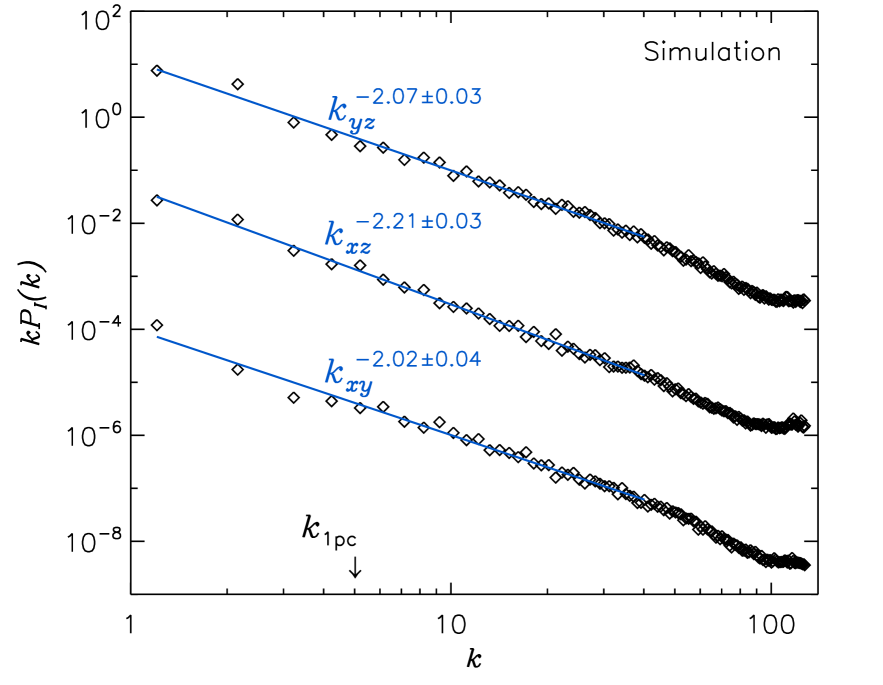
Before computing the power spectra, we apply a Gaussian beam with FWHM=$dx$, where $dx$ is the numerical mesh size, and add Gaussian noise to the synthetic spectra, to a level comparable to that of the FCRAO map of NGC 1333. The power spectra $P_{I}(k)$ and $P_{v}(k_{v})$ are shown for all three directions in Figures 1 and 2 respectively. $P_{I}(k)$ is very well described by a power law in the approximate range $1<k<50$ ($k=1$ corresponds to the linear size of the computational domain). Averaging the results of the three maps, we obtain the exponent $\beta_{I}=3.10\pm 0.08$, where the uncertainty is the standard deviation of the three measurements, a little larger than the standard deviation of each of the three individual least squares fits. In Padoan et al. (2006) we measured the same power spectrum, but without adding noise to the synthetic maps, and only in the direction of the x-axis. We obtained a slope of $2.99\pm 0.08$, consistent with the slope of $3.07$ found here for the same direction. This slope is also consistent with that of the density power spectrum measured directly from the three-dimensional snapshot, $\beta_{\rho}=3.0$.

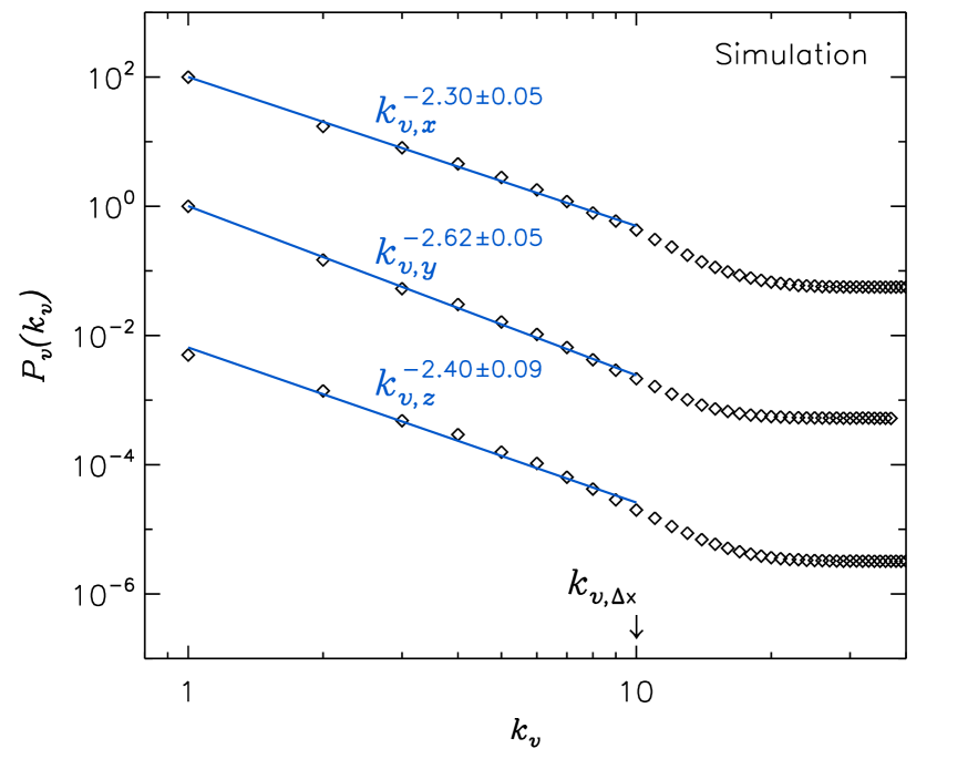
The least squares fits to the $P_{v}(k_{v})$ spectra are computed in the range $1<k_{v}<k_{v,\Delta x}$, where $k_{v,\Delta x}=256^{(\beta-1)/2}=10$, to satisfy the second condition for the validity of the VCS method. As shown in Figure 2, the power spectra $P_{v}(k_{v})$ are power laws up to $k_{v}\approx k_{v,\Delta x}$, and become steeper at larger values of $k_{v}$, as predicted by the theory. The steepening is here reduced by the effect of the added noise. Because the condition $\beta_{I}\geq 3$ is satisfied, we derive the energy spectrum from the relation $\beta=1+2/\beta_{v}$. We obtain $\beta=1.82\pm 0.04$, where the uncertainty is the standard deviation

of the exponents from the three maps. This result is consistent with the slope of 1.8 derived directly from the three-dimensional velocity field of the simulation snapshot. The value of $\beta_{I}$ is very close to the value of 3 that separates the regimes of steep and shallow density power spectra discussed in Lazarian and Pogosyan (2000, 2006). This is not a problem, because in the case of shallow density power spectra, the relation between $\beta$ and $\beta_{v}$ would be either the same or $\beta=1+2(\beta_{\rho}-2)/\beta_{v}$, depending on some other condition. The two formulas give the same result for $\beta_{\rho}\rightarrow 3$.

We conclude that the VCS method provides a precise estimate of the turbulent energy spectrum, by fitting the slope of $P_{v}(k_{v})$ for $k_{v}<k_{v,\Delta x}$. The $k_{v}$ range of the power law is limited. It is only a factor of 10 for the synthetic maps (and only a factor of 4 for the map of NGC 1333), because it is essentially given by the spatial dynamical range (256 for the synthetic maps) to the power $m/2=(\beta-1)/2$, as explained above. However, the average of the power spectra over many positions on the map ($256^{2}$ for both the synthetic maps and the map of NGC 1333), yields a $P_{v}(k_{v})$ spectrum that is extremely smooth and very well approximated by a power law, providing an accurate estimate of the slope of the turbulent energy spectrum.

We now apply the VCS method to the J=1-0 ¹³CO survey of the Perseus molecular cloud complex carried out with the FCRAO 14 m antenna by Ridge et al. (2006). The grid spacing of the survey is 23”, and the beam size 46”. The velocity-channel size is 0.06 km/s. We select a squared region of

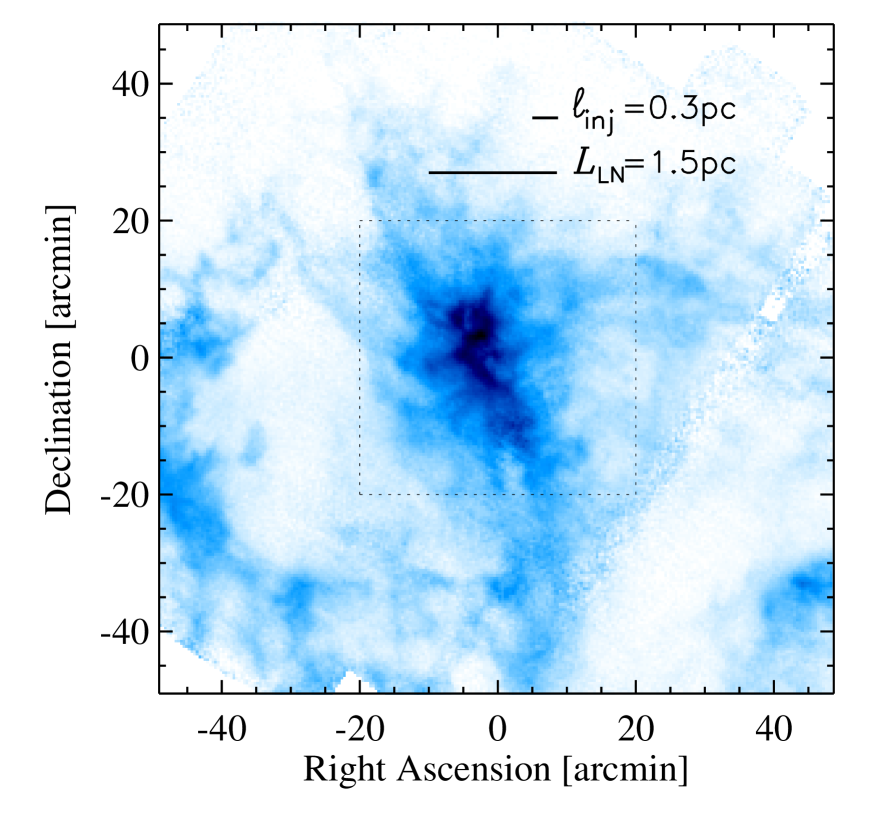
100$\times$100 arcmin, approximately centered on NGC 1333. This region contains $256\times 256$ spectra, like the synthetic maps. Figure 3 shows the integrated intensity map of that region. It also shows the size of $\ell_{\rm inj}=0.3$ pc and $L_{\rm LN}=1.5$ pc, the outflow injection scale and the size of the computational domain in Nakamura and Li (2007) and Carroll et al. (2009), assuming a distance to NGC 1333 of $D=280$ pc. For this distance, the size of the map is $S=7.9$ pc, the grid spacing 0.03 pc, and the beam size $\Delta x=0.06$ pc. The injection scale is therefore well resolved. The uncertainty on the distance to NGC 1333 is not very large, 220 pc$<D<$350 pc (Borgman and Blaauw 1964; Herbig and Jones 1983; Cernis 1990). Even assuming the largest value of $D=350$ pc, $\ell_{\rm inj}$ would still be 4 times larger than the beam size.

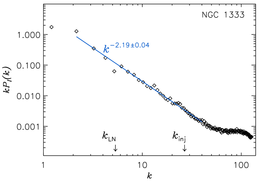
We compute the power spectra $P_{I}(k)$ and $P_{v}(k_{v})$ within that region, without any correction for the effects of beam and noise. This is justified because we do not compute the least squares fit at very large values of $k_{v}$ and $k$, and because we have confirmed the validity of the VCS method using synthetic maps where noise was added to a comparable level as in the map of NGC 1333. The $P_{I}(k)$ power spectrum is shown in Figure 4. The least squares fit, computed in the range $2\leq k\leq 40$, gives $\beta_{I}=3.19\pm 0.04$. The values of the wavenumbers $k_{\rm inj}$ and $k_{\rm LN}$, corresponding to the scales $\ell_{\rm inj}=0.3$ pc and $L_{\rm LN}=1.5$ pc, are marked by two arrows. The power spectrum is an almost perfect power law in the range of wavenumbers $1\leq k\leq 50$, corresponding to the range of scales 0.16 pc$<\ell<$7.9 pc ($k=1$ corresponds to the size of the map), with no significant feature around $\ell_{\rm inj}$.

Figure 5 shows the velocity coordinate power spectrum, $P_{v}(k_{v})$, and its least squares fit in the range $2\leq k_{v}\leq 8$, giving $\beta_{v}=2.34\pm 0.04$. This is the range of $k_{v}$ values expected from the VCS theory, because here $k_{v,\Delta x}=128^{(\beta-1)/2}=7.7$. As explained above, the dynamical range in $k_{v}$ is compressed with respect to that in $k$, as shown by the positions of $k_{v,\rm inj}$ and $k_{v,\rm LN}$, marked by two arrows. However, the measurement of the slope is still very accurate because the power spectrum is extremely smooth, as the result of averaging over the whole map, and very well represented by a power law. The injection scale falls in the very middle of the power law range, at $k_{v,\rm inj}=3.95$, and there is no sign of a variation of the slope within a range of values of $k_{v}$ corresponding to $\Delta x\leq\ell\leq L_{\rm LN}$, or 0.06 pc $\leq\ell\leq 1.5$ pc.

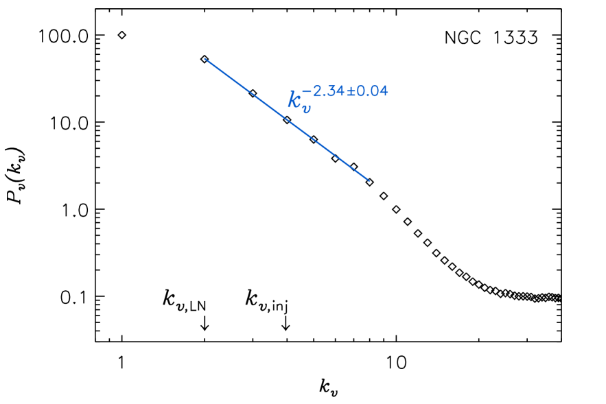
Using the relation $\beta=1+2/\beta_{v}$, we obtain $\beta=1.85\pm 0.02$, where the standard deviation is now derived directly by that of the least squares fit for $\beta_{v}$. This uncertainty may seem unrealistically small. Using the synthetic maps we have derived a standard deviation of 0.04 from the three values of $\beta$. If we instead derive the uncertainty directly from the standard deviation of each fit of $\beta_{v}$, we find that the average of the three uncertainty is 0.02, exactly like in the observational map. We therefore estimate that a more realistic uncertainty for the derived slope in NGC 1333 should be $\approx 0.04$.

To further verify this result, we also select a smaller region of $40\times 40$ arcmin ($3.2\times 3.2$ pc) around NGC 1333, shown as a dotted square in Figure 3. We obtain $\beta_{v}=2.29\pm 0.09$, corresponding to $\beta=1.87\pm 0.03$, consistent with the value estimated on the larger scale, though with a slightly larger uncertainty due to the smaller dynamical range and the smaller number of $P_{v}(k_{v})$ spectra in the map. The good consistency between the two maps is not surprising, because the sum of the $P_{v}(k_{v})$ spectra is dominated by the positions with the strongest integrated intensity that are mostly located within the inner map.

We conclude that the VCS method yields a turbulent energy power spectrum with slope $\beta=1.85\pm 0.04$, in the range of scales 0.06 pc $\leq\ell\leq 1.5$ pc, with no evidence of internal driving by outflows at the scale $\ell_{\rm inj}=0.3$ pc.

It has been suggested that protocluster clumps actively form stars for several dynamical times, while being supported by the turbulence internally generated by stellar outflows (e.g. Tan, Krumholz, and McKee 2006). This scenario is simulated by Nakamura and Li (2007) and Carroll et al. (2009), with physical parameters characteristic of NGC 1333. They find an energy injection scale, $\ell_{\rm inj}\approx 0.3$ pc, above which the turbulent energy spectrum is very shallow, up to the size of 1.5 pc of their computational domain. This value of $\ell_{\rm inj}$ and the flattening of the power spectrum above that scale are consistent with the results of the analytical model of Matzner (2007). If the turbulence in cluster-forming regions is primarily driven by outflows, the turbulent energy spectrum should flatten above the scale $\ell_{\rm inj}$, up to a scale where the external turbulent cascade dominates again.

We have searched for such a feature in the energy spectrum of NGC 1333, the prototype of outflow-driven regions in the cited theoretical works. To this aim, we have applied the VCS method of Lazarian and Pogosyan (2006) to the ¹³CO FCRAO map of NGC 1333, after successfully testing the method on simulated data. We have found the energy spectrum is a power law, $E(k)\propto k^{2}P_{v}(k)\propto k^{-\beta}$, with $\beta=1.85\pm 0.04$, in the range of scales 0.06 pc $\leq\ell\leq 1.5$ pc, with no evidence of internal driving by outflows at $\ell_{\rm inj}=0.3$ pc. The power spectrum of integrated intensity is also a power law, $P_{I}(k)\propto k^{-\beta_{I}}$, with $\beta_{I}=3.19\pm 0.04$, in the range of scales 0.16 pc$<\ell<$7.9 pc, with no significant features above the predicted injection scale.

These power spectra are consistent with those of large-scale driven simulations of supersonic turbulence, and with those measured on larger scale in Perseus and other molecular cloud complexes. Although outflows from young stars are present in NGC 1333, the large-scale turbulent cascade appears to be the main energy source. The turbulence in NGC 1333 is either currently driven by significant mass inflow from larger scales, or in the process of being dissipated, until the time when winds, outflows, and ionizing radiation from stars will completely disperse the star-forming gas.

References

- Borgman & Blaauw (1964) Borgman, J., & Blaauw, A. 1964, Bull. Astron. Inst. Netherlands, 17, 358
- Brunt et al. (2009) Brunt, C. M., Heyer, M. H., & Mac Low, M.-M. 2009, A&A, 504, 883
- Carroll et al. (2009) Carroll, J. J., Frank, A., Blackman, E. G., Cunningham, A. J., & Quillen, A. C. 2009, ApJ, 695, 1376
- Cernis (1990) Cernis, K. 1990, Ap&SS, 166, 315
- Colella & Woodward (1984) Colella, P., & Woodward, P. R. 1984, Journal of Computational Physics, 54, 174
- Heyer & Brunt (2004) Heyer, M. H., & Brunt, C. M. 2004, ApJ, 615, L45
- Herbig & Jones (1983) Herbig, G. H., & Jones, B. F. 1983, AJ, 88, 1040
- Juvela & Padoan (2005) Juvela, M., & Padoan, P. 2005, ApJ, 618, 744
- Kritsuk et al. (2007) Kritsuk, A. G., Norman, M. L., Padoan, P., & Wagner, R. 2007, ApJ, 665, 416
- Kritsuk et al. (2009) Kritsuk, A. G., Ustyugov, S. D., Norman, M. L., & Padoan, P. 2009, Astronomical Society of the Pacific Conference Series, 406, 15
- Kritsuk et al. (2009) Kritsuk, A. G., Ustyugov, S. D., Norman, M. L., & Padoan, P. 2009, Journal of Physics Conference Series, 180, 012020
- Krumholz & McKee (2005) Krumholz, M. R., & McKee, C. F. 2005, ApJ, 630, 250
- Lazarian & Pogosyan (2000) Lazarian, A., & Pogosyan, D. 2000, ApJ, 537, 720
- Lazarian & Pogosyan (2006) Lazarian, A., & Pogosyan, D. 2006, ApJ, 652, 1348
- Matzner (2007) Matzner, C. D. 2007, ApJ, 659, 1394
- Nakamura & Li (2007) Nakamura, F., & Li, Z.-Y. 2007, ApJ, 662, 395
- Norman & Bryan (1999) Norman, M. L., & Bryan, G. L. 1999, ASSL Vol. 240: Numerical Astrophysics, 19
- Padoan & Nordlund (2002) Padoan, P., & Nordlund, Å. 2002, ApJ, 576, 870
- Padoan & Nordlund (2004) Padoan, P., & Nordlund, Å. 2004, ApJ, 617, 559
- Padoan et al. (2004) Padoan, P., Jimenez, R., Juvela, M., & Nordlund, Å. 2004a, ApJ, 604, L49
- Padoan et al. (2006) Padoan, P., Juvela, M., Kritsuk, A., & Norman, M. L. 2006, ApJ, 653, L125
- Ridge et al. (2006) Ridge, N. A., et al. 2006, AJ, 131, 2921
- Tan et al. (2006) Tan, J. C., Krumholz, M. R., & McKee, C. F. 2006, ApJ, 641, L121