THE PRICING OF MULTIPLE-EXPIRY EXOTICS
Abstract.
In this paper we extend Buchen’s method to develop a new technique for pricing of some exotic options with several expiry dates (more than 3 expiry dates) using a concept of higher order binary option. At first we introduce the concept of higher order binary option and then provide the pricing formulae of -th order binaries using PDE method. After that, we apply them to get the pricing of some multiple-expiry exotic options such as Bermudan option, multi time extendable option, multiple shout option and etc. Here, when calculating the price of concrete multiple-expiry exotic options, we do not try to get the formal solution to corresponding initial-boundary problem of the Black-Scholes equation, but explain how to express the expiry payoffs of the exotic options as a combination of the payoffs of some class of higher order binary options. Once the expiry payoffs are expressed as a linear combination of the payoffs of some class of higher order binary options, in order to avoid arbitrage, the exotic option prices are obtained by static replication with respect to this family of higher order binaries.
Key words and phrases:
Multiple-expiry, Exotic option, Bermudan option, Extendable option, Shout option, Higher order Binary Option2010 Mathematics Subject Classification:
35C15, 91G801. Introduction
European and American options are referred to as vanilla options. Vanilla options have a single future expiry payoff that corresponds to buying or selling the underlying asset for a fixed amount called the strike price. European options can only be exercised at the expiry date, whereas American options may be exercised at any time before and at the expiry date. The various needs of risk management in financial markets give rise to many exotic (not ordinary) options with various payoff structures, and thus a lot of exotic options continue to be popular in the over-the counter market. Among them, there exists a class of exotic options whose payoff structure involves several fixed future dates, here we write them by . Usually, at the first expiry date , the option holder receives a contract related with dates . Options belonging to this class are called multiple-expiry exotic options. Bermudan options or several times extendable options are good examples.
In this paper we extend Buchen’s method [2] to develop a new technique for pricing of multiple expiry exotic options in terms of a portfolio of higher order binary options. An up (or down) binary option is the option that on its expiry date delivers an agreed payoff if the price of the underlying asset is above (or bellow) a fixed exercise price and zero otherwise. Binary options whose agreed payoff is an asset are referred as first order asset binaries and binary options whose agreed payoff is cash are referred as first order bond binaries [2]. In this paper, the binary options whose agreed payoff is a -th order binary are called -th order binaries by induction.
The basic idea of expressing the payoffs of complex options in terms of binary options can be seen in previous publications. Rubinstein and Reiner [7] considered the relationship of barrier options and binaries. Ingersoll [3] extended the idea by expressing complex derivatives in terms of ”event-driven” binaries. Event -driven binary option pays one unit of underlying asset if and only if the event occurs, otherwise it pays nothing.
Buchen [2] developed a theoretical framework for pricing dual-expiry options in terms of a portfolio of elementary binary options. He introduced the concepts of first and second order binary options and provided the pricing formula for them using expectation method. And then he applied them to pricing some dual expiry exotic options including compound option, chooser option, one time extendable option, one time shout option, American call option with one time dividend and partial barrier options.
The purpose of this paper is to extend the Buchen’s procedure to the case of multiple-expiry options (more than 3 expiry dates). To do that, here, at first we introduced the concept of higher order binary options and then provided the pricing formula of -th order binaries using PDE method. After that, we applied them to pricing of some multiple-expiry exotic options such as Bermudan options, multi time extendable options, multiple shout options and etc.
As Buchen [2] mentioned, historically, dual expiry exotics as well as multiple-expiry option prices have been derived individually by various authors. This paper has demonstrated that multiple-expiry options can be priced in a unified framework by expressing each as a portfolio of higher order binaries.
The focus of this paper is on explaining the basic pricing method in terms of static replication with higher order binaries, and so issues such as the financial motivation for trading multiple-expiry exotics, computation and simulation will not be considered here in detail and the explanation about another authors’ results on concrete multiple-expiry exotics such as Bermudan option, extendable option and shout option will refer to [6, 9, 10].
2. Higher Order Binary Options
Consider an underlying asset (for example, a stock) whose price satisfies Ito stochastic differential equation. Let and be respectively risk free rate, dividend rate and volatility. Then to avoid arbitrage, the price of of any derivative on the stock with expiry date and expiry payoff must satisfy the following (1)-(2).
| (1) |
| (2) |
This price is called a standard option with expiry payoff [2].
Proposition 1[5] Assume that there exist non negative constants and such that . Then the price of standard option, that is, the solution of (1) and (2) is provided as follows:
| (3) |
Remark. It is well known that the change of variable transforms (1) to a parabolic PDE with constant coefficients which can be easily transformed into a heat equation. (For example, see [4].) From the theory of heat equations we can know that the singular integral on the left side of (3) and its and derivatives always exist under the above condition on , which can be easily seen in references such as [8] on PDE or equations of mathematical physics, and we can easily check that (3) satisfies (1) and (2).
An up binary option of exercise price on the standard option with expiry payoff is a contract with expiry payoff if and zero otherwise. A down binary option pays if and zero otherwise. Let be the sign ”” or ””. In what follows we use the sign ”” and ”” as sign indicators for up and down binaries, respectively. Then the expiry payoff functions for up and down binaries can be written in the form
From this there holds the following parity relation between the standard option price and the corresponding up and down binaries:
If , the standard option simply pays one unit of the asset at expiry date , and the price of the standard option is for all . And the corresponding binaries are the very asset-or-nothing binaries, here their prices are denoted by . Then from the above mentioned parity relation, we have
If , the standard option simply pays one unit of cash at expiry date , and the price of the standard option is for all . And the corresponding binaries are the very cash-or-nothing binaries (or bond binaries), here their prices are denoted by . From the parity relation, we have
The concept of Q-option plays a very useful role in the pricing of dual expiry options and, in particular, simplifying the notation of the price formula. (See [2].) Consider a standard contract that pays at expiry date ; this is a kind of forward contract, where the holder must buy if (or sell if ) one unit of underlying asset for units of cash. Since , the price of this contract at time is given by
The binary option that pays at expiry date is called a first order Q-option, their prices denoted by . If , then is is the very ordinary European (call if , or put if ) option. So is called a generalized European option. These options are more general in the sense that their exercise price is different from their strike price . The price of first order Q-options are given as follows:
| (4) |
The asset or nothing binary, bond binary and the first order Q-option are called the first order binaries.[2]
Proposition 2[2, 4]. The prices of asset and bond binary options are provided as follows:
| (5) |
Here is the accumulated normal distribution function
and , are respectively given as follows:
Definition 1. An -th order binary option is a binary contract with expiry date on an underlying -th order binary option. Specifically, the payoff at time has the following form
| (6) |
Here is the price of the underlying -th order binary option with expiry time at the time and either if the underlying binary is asset binary, for the underlying bond binary or for the underlying -option; and are up-down indicators ( or ) at times respectively. are their corresponding exercise prices.
The prices of these -th order binary options at time are denoted by .
Then from the definition we have
=
| (7) |
Note that the strike price in the higher order -binary is effective only at last time . From the parity relation, we have
If the pricing formulae of the higher order asset binary and the higher order bond binary are provided, then the price of the higher order -binary is easily provided by (7).
Black-Scholes expressions for higher order binary options involve multidimensional normal distribution function with zero mean vector and correlation matrix :
| (8) |
Here
Let define the matrix related to the expiry dates as follows:
,
,
,
,
and another elements are all zero. Then we have
Let or (that is, sign indicators and ) and define a new matrix by
Then we have
Theorem 1 The price of -th order asset binary and bond binary are provided as follows :
| (9) |
| (10) |
Here
Proof: The cases of and were proved by Buchen in [2] using probability theory and can be easily proved using the formula (3) too. In the case of we will give a sketch of the proof by induction.
We assume that theorem 1 holds in the case of . From the definition 1, satisfies (1) and
Therefore by the formula (3), If we let
then is provided as follows:
.
Here is the price of the underlying -th order asset binary option. By induction-assumption, the formula (9) holds for . Thus we have
Substitute this equality into the above singular integral representation and calculate the integral, then we have (9) for the case of . The proof for (10) is similar. (Proof End)
The formulae (7), (9) and (10) give the following price of higher order -option :
| (11) |
3. Applications to Multiple-Expiry Exotics
In this section, we applied the results of previous section to the pricing of some multiple expiry exotics.
The Static Replication Theorem If the payoff of an option at expiry time is a linear combination of prices at time of higher order binaries, then its price at all time is the combination of the corresponding prices at time of the higher order binaries.
The static replication theorem can be proved from the uniqueness of solution to the initial value problem of Black-Scholes equation. And we need one lemma that guarantees the monotonousness of the option price on the underlying asset price and provides some estimates about the gradient of the price on the underlying asset price.
Lemma 1 Assume that is continuous and piecewise differentiable. If is the solution of (1) and (2), then we have
In particular, if and , then
Using the formula (3) and the assumption of lemma 1, we can easily prove the required results.
3.1. Bermudan Options
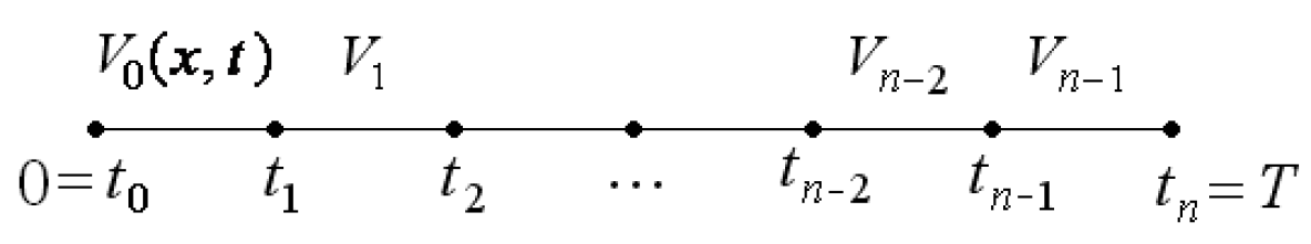
The Bermudan option is one type of nonstandard American options and early exercise is restricted to certain dates during the life of the option. For example, let be the dates of early exercise for put option with strike price . Let . Let denote the option price on the interval by , where . Then [4]
| (12) |
(See figure 1.)
For fixed , we consider the following equation:
| (13) |
If is monotonously decreasing on , and , then the equation (13) has a unique root such that . (See figure 2.)
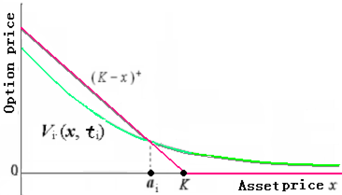
Lemma 2 Fix . Assume that is monotonously decreasing on , and . Let be the unique root of the equation (13). Then for any , we have
and . In particular, if , then . Here is the solution of Black-Scholes equation (1) satisfying the condition .
Proof. From the assumption, we can rewrite (12) as follows. (See figure 2.)
Thus from the definition of the binary option, we have
From the assumption we have and thus using lemma 1, we have the conclusion on . (Proof End)
Using this lemma, we can easily calculate the price of Bermudan put options. Since the payoff at time is and we can’t early exercise after the time , so the option on the interval becomes an ordinary European put option, and thus its price in the interval is given by
and satisfies and . By the static replication theorem and lemma 2, our option price at time is given by
and . Repeating the similar considerations, we can get the following formulae:
| (14) |
In particular, gives the price of Bermudan put option at time .
3.2. Multiple Extendable Options
Extendable options were first studied and analyzed in detail by Longstaff [6]. Here we consider the holder extendable options in his sense. The holder -times extendable call (or put) option has the right at some certain dates to exercise a standard European call (or put) option of strike price or to extend the expiry date to time and change the strike price from to for a premium . Here we consider -times extendable call option.
Let denote the option price on the interval by , where and . Then from the definition of extendable option, we have
| (15) |
First, let consider the price in the last interval . In this interval we can no longer extend our option contract and thus our option is just an ordinary European call with the expiry date and strike price . Therefore
And it satisfies by lemma 1.
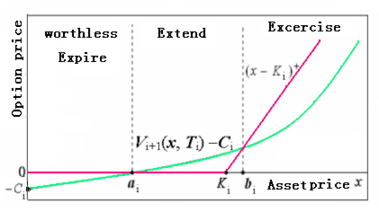
Now consider the price in the interval . Then by (15) we have
From the property of , the following two equations on have unique roots and , respectively.
| (16) |
And it is quite natural that we assume that . (Otherwise the extension of to would not occur as Buchen [2] mentioned. See figure 3. Similarly, in put we assume that .)
Then we can rewrite as follows:
Thus using the Static Replication Theorem, for we have
.
And is a monotone increasing function of with a positive inclination less than 1 in . (See figure 3.) By lemma 1, we have
By similar consideration and induction, we can prove that the formula of price of our option in the time interval is provided by
| (17) |
Here is the or indicator, that is,
In particular gives the price of n-times extendable call option in the time interval .
3.3. Multiple Shout Options
Shout options (Thomas [10]) are exotic options that allow the holder to lock in a payoff at times prior to the final expiry date. If the shout times would be selected randomly according to the holder’s mind, the pricing of shout option will be quite challenging, but if the shout times are pre-determined, then it would be simpler ([2]). In a fixed time multiple shout call option with expiry date and strike price , their payoff can be locked in at some predetermined times . So at the final expiry date , its payoff is given as follows:
| (18) |
where are the underlying asset price at the shout time .
For simplicity, here we consider the case . Then the expiry payoff (18) is given by
| (19) |
Note that in the last interval both of the underlying asset prices and are known constants and in the interval the underlying asset price is a known constant.
The case of . We can rewrite (19) as
and this is the terminal payoff of one-shout option in the time interval and thus by the method of [2], for we have
Here
| (20) |
In particular at the time , we have
| (21) |
The case of . If , then we can rewrite (19) as follows:
Thus in the time interval we have
In particular, at the time and
where is as in (20). Thus
| (22) |
If , then we can rewrite (19) as follows:
Thus in the time interval we have
In particular, at the time
| (23) |
Combining (22) with (23) to get
Note that in the interval the underlying asset price is a known constant. Then using the Static Replication Theorem, for , we have
4. Conclusions
In this paper we introduced the concept of higher order binary options and then provide the pricing formulae of -th order binaries using solving method of PDE. Then we applied them to pricing of some multiple-expiry exotic options such as Bermudan options, multi time extendable options, fixed time twice shout options and etc. Here when calculating the price of concrete multiple-expiry exotic options, the focus of discussion was on explaining how to express the expiry payoffs of the exotic option as a combination of the payoffs of some class of higher order binary options. Here we assumed that risk free rate, dividend rate and volatility are constant but we could easily extend to the case with time dependent coefficients.
References
- [1] Broadie, M. and Yamamoto Y., Application of the Fast Gauss Transform to option pricing, Management science, Vol. 49, No. 8, 1071-1088, 2003
- [2] Buchen, P., The Pricing of dual-expiry exotics, Quantitative Finance, 4, 101-108, 2004
- [3] Ingersoll, J. E., Digital contract: simple tools for pricing complex derivatives, J. Business, 73, 67-88, 2000
- [4] Jiang, Li-shang, Mathematical Modeling and Methods of Option Pricing, World Scientific, Singapore, 2005
- [5] Kwok, Y.K., Mathematical models of Financial Derivatives, Springer-verlag, Berlin, 55-82, 1999
- [6] Longstaff, F., Pricing options with extendable maturities: analysis and applications, J. Finance, 45, 935-957, 2000.
- [7] Rubinstein, M. and Reiner, E., Unscrambling the binary code, Risk Mag. 4, 75-83, 1991
- [8] Rubinstein, I. and L. Rubinstein, Partial Differential Equations in Classical Mathematical Physics, Cambridge Univ. Press, 296-324, 1998
- [9] Schweizer, M., On Bermudan Options, Advances in Finance and Stochastics, in Essays in Honor of Dieter Sondermann, Springer, 257-269, 2002
- [10] Thomas, B., Something to shout about, Risk Mag. 6, 56-58, 1994