The Principal Fiber Bundle Structure of the Gimbal-Spacecraft System

Spacecrafts are actuated by two principles - internal or external actuation. The actuators in the former class consist of momentum wheels (also called internal rotors) and control moment gyros (CMGs). A refinement of CMGs are the variable speed CMGs (called VSCMGs). Examples of external actuation systems include gas jet thrusters mounted on the outer body of the spacecraft. In this article we focus on spacecraft with gimbals (or the VSCMG) as the mechanism of actuation.

The modelling of a spacecraft with a VSCMG has been reported in the literature schaub_feedback_1998 ; schaub_singularity_2000 . Studies on singularity issues of this system are found in tsiotras_singularity_2004 ; schaub_singularity_2000 . Control law synthesis and avoidance of singularities are found in bedrossian_thesis_1987 ; margulies_aubrun_1978 ; schaub_singularity_2000 ; tsiotras_singularity_2004 An early study of singularity in a geometric framework is kurokawa_geometric_1998 . That study considers possibility of avoiding singular gimbal angle configurations using global control. The analysis proceeds by considering the inverse images of CMG system angular momenta as union of sub“manifolds” of the n-dimensional gimbal angle configuration space. The nature of these manifolds are examined at and near singular gimbal configurations.

Spurred by the insight and creativity of J. E. Marsden marsden2013introduction ,the geometric mechanics community bloch_nonholo_mech_ctrl ; ostrowski1999computing has studied very many mechanical systems in the geometric framework. This framework has proved beneficial in providing insight into these systems and their structure by preserving the mechanical objects (momentum, energy) of these systems and also proving useful in control design bloch2001controlledlagrangian ; bloch2000controlled .

A geometric description of the VSCMG system based on variational principles is studied in sanyal2013vscmg . The configuration space of the system is shown to be a principal fiber bundle and the expression for the Ehressmann connection is derived. The paper considers a general system where the rotor mass centre is offset from the gimbal axis. A stabilising control law is derived as a function of the internal momentum. Singularity analysis of this system under typical simplifying assumptions is explored in sanyal2015vscmg . The system is discretised into a model which preserves the conserved quantities using variational integrators.

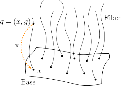
While studying the problem of interconnected mechanical systems, the geometry of the configuration space which is a differential manifold requires attention for elegant and insightful solutions. This configuration space $Q$, is often written as the product of two manifolds. One component is the base manifold $M$, which in our context describes the configuration of the gimbals mounted inside the spacecraft. The other component of the configuration variables depicting the attitude of the spacecraft is a Lie group $G$, in this case $\mathop{\mathbb{SO}(3)}$ boothby1975introduction . The total configuration space of the spacecraft $Q$ then naturally appears as a product $G\times M$. Such systems follow the topology of a trivial principal fiber bundle, see kobayashi1963foundations . Figure 1 shows an explanatory figure of a fiber bundle. The components of the 2-tuple $q=(x,g)$ denote the base and the group variable respectively. The projection map $\pi:Q\mathop{\rightarrow}M$ maps the configuration space to the base space. With such a separation of the configuration space, locomotion is readily seen as the means by which changes in shape affect the macro position. We refer to kelly1995geometric ; bloch_nonholo_mech_ctrl for a detailed explanation on the topology of locomoting systems.

In this article we present a completely geometric approach to the modelling of the VSCMG-spacecraft system and relate it to a conventional modelling approach.

The configuration space of the spacecraft-gimbal system (with one CMG) is $Q=\mathop{\mathbb{SO}(3)}\times\mathbb{S}^{1}\times\mathbb{S}^{1}$ and any arbitrary configuration is expressed by the 3-tuple $(R_{s},\beta,\gamma)$, where the first element denotes the attitude $R_{s}$ of the spacecraft with respect to fixed / inertial frame, the second denotes the degree of freedom $\beta$ of the gimbal frame, the third denotes the degree of freedom $\gamma$ of the rotor about its spin axis. For the purpose of later geometrical interpretation, we club $x\stackrel{{\scriptstyle\triangle}}{{=}}(\beta,\gamma)$. There are three rigid bodies involved here, each having relative motion (rotation) about the other. Therefore, three frames of reference are chosen (apart from the inertial frame) - the first is the spacecraft, denoted by the subscript $s$, the second is the gimbal frame, denoted by the subscript $g$, the third is the rotor frame, denoted by the subscript $r$. The moments of inertia of the homogeneous rotor and the gimbal in their respective body frames are assumed to be

$\displaystyle\mathbb{I}_{r}=\begin{pmatrix}J_{x}&0&0\\ 0&J_{x}&0\\ 0&0&J_{z}\end{pmatrix}\;\;\;\mathbb{I}_{g}=\begin{pmatrix}I_{t}&0&0\\ 0&I_{g}&0\\ 0&0&I_{s}\end{pmatrix}$

(1)

Since the rotor is assumed to be homogeneous and symmetric, its inertia is represented in the gimbal frame and the combined gimbal-rotor inertia is rewritten as

$\displaystyle\mathbb{I}_{gr}=\begin{pmatrix}(J_{x}+I_{t})&0&0\\ 0&(J_{x}+I_{g})&0\\ 0&0&(J_{z}+I_{s})\end{pmatrix}$

(2)

If the rotational transformation that relates the gimbal frame to the spacecraft frame is given by $R_{\beta}$, where $\beta$ denotes the gimballing angle, then the gimbal-rotor inertia reflected in the spacecraft frame is

$\displaystyle(\mathbb{I}_{gr})_{\beta}\stackrel{{\scriptstyle\triangle}}{{=}}R_{\beta}\mathbb{I}_{gr}R_{\beta}^{T}$

(3)

Here the subscript $\beta$ denotes the dependance on the gimbal angle $\beta$.

To arrive at the dynamic model we proceed as follows. From the expression for the total momentum

	$\displaystyle\mu$	$\displaystyle=Ad_{R_{s}^{T}}^{*}[((\mathbb{I}_{gr})_{s}+\mathbb{I}_{s})\Omega_{s}+R_{\beta}\mathbb{I}_{gr}\begin{pmatrix}0\\ \dot{\beta}\\ \dot{\gamma}\end{pmatrix}]$
		$\displaystyle=R_{s}\begin{pmatrix}\tilde{\mathbb{I}}(x)&R_{\beta}\mathbb{I}_{gr}\end{pmatrix}\begin{pmatrix}\Omega_{s}\\ \begin{pmatrix}0\\ \dot{\beta}\\ \dot{\gamma}\end{pmatrix}\end{pmatrix}$		(25)

We split the momentum in to two components - one due to the gimbal-rotor unit and the other due to the rigid spacecraft. Further, we assume an internal torque $\tau_{b}$ (in the gimbal-rotor frame), generated by a motor, acts on the gimbal and rotor unit. We then have, due to the principle of action and reaction

$\displaystyle\frac{d}{dt}(R_{s}\mathbb{I}_{s}\Omega_{s})=\underbrace{-R_{s}\tau_{b}}_{reaction}\;\;\;\;\;\;\frac{d}{dt}(R_{s}[R_{\beta}\mathbb{I}_{gr}R_{\beta}^{T}\Omega_{s}+R_{\beta}\mathbb{I}_{gr}\dot{x}])=\underbrace{R_{s}\tau_{b}}_{action}$

(26)

The detailed computation is now shown. Differentiating $\mu=R_{s}R_{\beta}\mathbb{I}_{gr}(R_{\beta}^{T}\Omega_{s}+\begin{bmatrix}0\\ \dot{\beta}\\ \dot{\gamma}\end{bmatrix})$ with respect to time, we have $\frac{d}{dt}\mu_{cmg}=\frac{d}{dt}\left\{R_{s}R_{\beta}\mathbb{I}_{gr}(R_{\beta}^{T}\Omega_{s}+\begin{bmatrix}0\\ \dot{\beta}\\ \dot{\gamma}\end{bmatrix})\right\}=\text{torque acting on cmg external to cmg}$

$\tau_{extcmg}=\left\{\begin{array}[]{c}(R_{s}\hat{\Omega}_{s})R_{\beta}\mathbb{I}_{gr}(R_{\beta}^{T}\Omega_{s}+\begin{bmatrix}0\\ \dot{\beta}\\ \dot{\gamma}\end{bmatrix})\\ +R_{s}(R_{\beta}\hat{i}_{2}\dot{\beta})\mathbb{I}_{gr}(R_{\beta}^{T}\Omega_{s}+\begin{bmatrix}0\\ \dot{\beta}\\ \dot{\gamma}\end{bmatrix})\\ +R_{s}R_{\beta}\mathbb{I}_{gr}(-\hat{i}_{2}R_{\beta}^{T}\dot{\beta}\Omega_{s})\\ +R_{s}R_{\beta}\mathbb{I}_{gr}(R_{\beta}^{T}\dot{\Omega}_{s})\\ +R_{s}R_{\beta}\mathbb{I}_{gr}(\begin{bmatrix}0\\ \ddot{\beta}\\ \ddot{\gamma}\end{bmatrix})\end{array}\right\}$

	$\displaystyle\tau_{extcmg}={}$	$\displaystyle R_{s}\hat{\Omega}_{s}R_{\beta}\mathbb{I}_{gr}(R_{\beta}^{T}\Omega_{s}+\begin{bmatrix}0\\ \dot{\beta}\\ \dot{\gamma}\end{bmatrix})$
		$\displaystyle+R_{s}R_{\beta}\left\{\hat{i}_{2}\dot{\beta}\mathbb{I}_{gr}(R_{\beta}^{T}\Omega_{s}+\begin{bmatrix}0\\ \dot{\beta}\\ \dot{\gamma}\end{bmatrix})+\mathbb{I}_{gr}(-\hat{i}_{2}R_{\beta}^{T}\dot{\beta}\Omega_{s})+\mathbb{I}_{gr}(\begin{bmatrix}0\\ \ddot{\beta}\\ \ddot{\gamma}\end{bmatrix})\right\}$

In the spacecraft body coordinates,

	$\displaystyle\tau_{extcmg}^{\mathcal{B}}={}$	$\displaystyle\hat{\Omega}_{s}R_{\beta}\mathbb{I}_{gr}(R_{\beta}^{T}\Omega_{s}+\begin{bmatrix}0\\ \dot{\beta}\\ \dot{\gamma}\end{bmatrix})$
		$\displaystyle+R_{\beta}\left\{\hat{i}_{2}\dot{\beta}\mathbb{I}_{gr}(R_{\beta}^{T}\Omega_{s}+\begin{bmatrix}0\\ \dot{\beta}\\ \dot{\gamma}\end{bmatrix})+\mathbb{I}_{gr}(-\hat{i}_{2}R_{\beta}^{T}\dot{\beta}\Omega_{s})+\mathbb{I}_{gr}(\begin{bmatrix}0\\ \ddot{\beta}\\ \ddot{\gamma}\end{bmatrix})\right\}$

Defining two vectors

	$\displaystyle u_{1}={}$	$\displaystyle\mathbb{I}_{gr}(R_{\beta}^{T}\Omega_{s}+\begin{bmatrix}0\\ \dot{\beta}\\ \dot{\gamma}\end{bmatrix})$
	$\displaystyle u_{2}={}$	$\displaystyle\left(\hat{i}_{2}\mathbb{I}_{gr}-\mathbb{I}_{gr}\hat{i}_{2}\right)R_{\beta}^{T}\Omega_{s}\dot{\beta}+\hat{i}_{2}\mathbb{I}_{gr}\begin{bmatrix}0\\ \dot{\beta}\\ \dot{\gamma}\end{bmatrix}\dot{\beta}+\mathbb{I}_{gr}(\begin{bmatrix}0\\ \ddot{\beta}\\ \ddot{\gamma}\end{bmatrix})$

in the gimbal frame $\mathcal{G}$ such that $\tau_{extcmg}^{\mathcal{B}}=\hat{\Omega}_{s}R_{\beta}u_{1}+R_{\beta}u_{2}$ . The second component of this vector gives the torque acting on the gimbal motor and the third gives the torque acting on the wheel motor. We now simplify this expression to obtain more explicit equations, which we then compare with a standard model existing in the literature.

$$[\hat{\Omega}_{s}\tilde{\mathbb{I}}(x)\Omega_{s}+\tilde{\mathbb{I}}(x)\dot{\Omega}_{s}]$$

$\displaystyle=(-1)\hat{\Omega}_{s}R_{\beta}\mathbb{I}_{gr}\dot{x}-\dot{\beta}R_{\beta}{\cal U}R_{\beta}^{T}\Omega_{s}-\dot{\beta}R_{\beta}\hat{i}_{2}\mathbb{I}_{gr}\dot{x}-R_{\beta}\mathbb{I}_{gr}\ddot{x}$

(27)

where ${\cal U}\stackrel{{\scriptstyle\triangle}}{{=}}\hat{i}_{2}\mathbb{I}_{gr}-\mathbb{I}_{gr}\hat{i}_{2}$ is a symmetric matrix.

We now draw connections between the approach outlined in the previous sections with that of the classical CMG modeling and analysis done in the Newtonian framework in schaub_feedback_1998 , which is cited in much of the aerospace literature. We shall refer to this paper as the SRJ paper henceforth. We first relate the notation and then establish a connection with the main equations of the SRJ paper.

The two primary variables in the SRJ paper and ours are related as in table 1.

The rotation matrix in the SRJ paper, relating the gimbal and spacecraft-body frame, is described in terms of three orthogonal column vectors of unit norm, $\{\hat{g}_{s},\hat{g}_{t},\hat{g}_{g}\}$, where the subscripts $s,t$ and $g$ correspond to the spin, transverse and gimbal axes, as

$\displaystyle\begin{pmatrix}|&|&|\\ \hat{g}_{s}&\hat{g}_{t}&\hat{g}_{g}\\ |&|&|\\ \end{pmatrix}$

(28)

and further,

$\displaystyle\begin{pmatrix}\left\langle{\hat{g}_{s}},{\omega}\right\rangle\\ \left\langle{\hat{g}_{t}},{\omega}\right\rangle\\ \left\langle{\hat{g}_{g}},{\omega}\right\rangle\end{pmatrix}=\begin{pmatrix}\omega_{s}\\ \omega_{t}\\ \omega_{g}\end{pmatrix}$

(29)

In our convention, the following correspondence holds:

$\displaystyle R_{\beta}=\begin{pmatrix}|&|&|\\ \hat{g}_{t}&\hat{g}_{g}&\hat{g}_{s}\\ |&|&|\\ \end{pmatrix}$

(30)

and

$\displaystyle R_{\beta}^{T}\Omega_{s}\longrightarrow\begin{pmatrix}\omega_{t}\\ \omega_{g}\\ \omega_{s}\end{pmatrix}$

(31)

The SRJ equation of motion (eqn. 28) written partially in terms of our notation is

$\displaystyle\tilde{\mathbb{I}}(x)\dot{\Omega}_{s}+\hat{\Omega}_{s}\tilde{\mathbb{I}}(x)\Omega_{s}=$

(32)

$\displaystyle-\hat{g}_{s}[J_{s}(\ddot{\gamma}+\dot{\beta}\omega_{t})-(J_{t}-J_{g})\omega_{t}\dot{\beta}]-\hat{g}_{t}[J_{s}(\dot{\gamma}+\omega_{s})\dot{\beta}-(J_{t}+J_{g})\omega_{s}\dot{\beta}+J_{s}\dot{\gamma}\omega_{g}]-\hat{g}_{g}[J_{g}\ddot{\beta}-J_{s}\dot{\gamma}\omega_{t}]$

(33)

while the RHS of the same equation in our notation is

$$-[\hat{\Omega}_{s}+\dot{\beta}\hat{i}_{2}]R_{\beta}\mathbb{I}_{gr}\dot{x}-\dot{\beta}R_{\beta}(\hat{i}_{2}\mathbb{I}_{gr}-\mathbb{I}_{gr}\hat{i}_{2})R_{\beta}^{T}\Omega_{s}-R_{\beta}\mathbb{I}_{gr}\ddot{x}$$

$$=-\hat{g}_{t}[(J_{z}+I_{s})\dot{\gamma}\dot{\beta}-(J_{x}+I_{g})\dot{\beta}\omega_{s}+(J_{z}+I_{s})\dot{\gamma}\omega_{g}+(J_{z}+I_{s})-(J_{x}+I_{t})\dot{\beta}\omega_{s}]$$

$$-\hat{g}_{g}[(J_{x}+I_{g})\ddot{\beta}-(J_{z}+I_{s})\dot{\gamma}\omega_{t}]$$

$$-\hat{g}_{s}[(J_{z}+I_{s})\ddot{\gamma}+(J_{x}+I_{g})\dot{\beta}\omega_{t}+((J_{z}+I_{s})-(J_{x}+I_{t}))\dot{\beta}\omega_{t}]$$

The terms in the model expand as shown below.

	$\displaystyle R_{\beta}\mathbb{I}_{gr}[0,\ddot{\beta},\ddot{\gamma}]^{T}$	$\displaystyle=\vec{g}_{g}(J_{x}+I_{g})\ddot{\beta}+\vec{g}_{s}(J_{z}+I_{s})\ddot{\gamma}$
	$\displaystyle R_{\beta}\hat{i}_{2}\dot{\beta}\mathbb{I}_{gr}[0,\dot{\beta},\dot{\gamma}]^{T}$	$\displaystyle=\vec{g}_{t}(J_{z}+I_{s})\dot{\gamma}\dot{\beta}$
	$\displaystyle\hat{\Omega}_{s}R_{\beta}\mathbb{I}_{gr}[0,\dot{\beta},\dot{\gamma}]^{T}$	$\displaystyle=\begin{array}[]{c}\vec{g}_{s}((J_{x}+I_{g})\dot{\beta}\omega_{t})+\vec{g}_{g}(-(J_{z}+I_{s})\dot{\gamma}\omega_{t})\\ \vec{g}\left(-(J_{x}+I_{g})\dot{\beta}\omega_{s}+(J_{z}+I_{s})\dot{\gamma}\omega_{g}\right)\end{array}$
	$\displaystyle\hat{i}_{2}\mathbb{I}_{gr}-\mathbb{I}_{gr}\hat{i}_{2}$	$\displaystyle=\begin{bmatrix}0&0&\left(J_{z}+I_{s}-(J_{x}+I_{t})\right)\\ 0&0&0\\ \left(J_{z}+I_{s}-(J_{x}+I_{t})\right)&0&0\end{bmatrix}$
	$\displaystyle R_{\beta}(\hat{i}_{2}\mathbb{I}_{gr}-\mathbb{I}_{gr}\hat{i}_{2})R_{\beta}^{T}\Omega_{s}\dot{\beta}$	$\displaystyle=(\vec{g}_{t}\omega_{s}+\vec{g}_{s}\omega_{t})(\left\{J_{z}+I_{s}-(J_{x}+I_{t})\right\}\dot{\beta})$

We now detail the explicit computation of the connection form. The principal fiber bundle structure introduces a vertical space in the tangent space at each point on the manifold. The vertical space consists of those vectors corresponding to the infinitesimal generator vector fields at that particular point. The tangent space is then expressed as the direct sum of the vertical space and a horizontal space, where the horizontal space gets defined as the subspace orthogonal to the vertical space in the inner product induced by the Riemannian metric.

The expression for the kinetic energy is

$$[\Omega^{T}\ u_{1}\ u_{2}]\begin{bmatrix}\mathbb{I}_{s}+R_{\beta}\mathbb{I}_{gr}R_{\beta}^{T}&(J_{x}+I_{g})\vec{g}&(J_{z}+I_{s})\vec{s}_{\beta}\\ (J_{x}+I_{g})\vec{g}^{T}&(J_{x}+I_{g})&0\\ (J_{z}+I_{s})\vec{s}_{\beta}^{T}&0&(J_{z}+I_{s})\end{bmatrix}\begin{bmatrix}\Xi\\ w_{1}\\ w_{2}\end{bmatrix}$$

Action and infinitesimal generator are as shown in other sections. So vertical space at a point $q$ is spanned by $\{(\square,0,0)|\square\in T_{q}SO(3)\}$. Locally we can represent elements in $T_{q}Q$ as $((r_{1},\ r_{2},\ r_{3}),\ \dot{\beta},\ \dot{\gamma})$ where $(r_{1},\ r_{2},\ r_{3})\in\mathbb{R}^{3}\simeq\mathfrak{so}(3)$.Then

$$V_{q}Q=\mathrm{span}\{\frac{\partial}{\partial r_{1}},\ \frac{\partial}{\partial r_{2}},\ \frac{\partial}{\partial r_{3}}\}$$

To find, $H_{q}Q$, the $\mathbb{G}$ orthogonal space has to be found out.

$$\left\langle\begin{bmatrix}\mathbb{I}_{s}+R_{\beta}\mathbb{I}_{gr}R_{\beta}^{T}&(J_{x}+I_{g})\vec{g}&(J_{z}+I_{s})\vec{s}_{\beta}\\ (J_{x}+I_{g})\vec{g}^{T}&(J_{x}+I_{g})&0\\ (J_{z}+I_{s})\vec{s}_{\beta}^{T}&0&(J_{z}+I_{s})\end{bmatrix}\begin{bmatrix}\begin{pmatrix}h_{1}\\ h_{2}\\ h_{3}\end{pmatrix}\\ h_{4}\\ h_{5}\end{bmatrix},\quad\begin{bmatrix}\square\\ 0\\ 0\end{bmatrix}\right\rangle=0$$

where $\square\in V_{q}Q$ . This implies

$$(\mathbb{I}_{s}+R_{\beta}\mathbb{I}_{gr}R_{\beta}^{T})\begin{pmatrix}h_{1}\\ h_{2}\\ h_{3}\end{pmatrix}+(J_{x}+I_{g})\vec{g}h_{4}+(J_{z}+I_{s})\vec{s}_{\beta}h_{5}=0$$

The horizontal vector $(h_{1}\ h_{2}\ h_{3}\ h_{4}\ h_{5})^{T}$ satisfies 3 (independent) equations in 5 variables. The horizontal space is then 2 dimensional as expected since the number of shape variables is 2. If we let $h_{4}$ and $h_{5}$ be the independent variables, then

	$\displaystyle\begin{pmatrix}h_{1}\\ h_{2}\\ h_{3}\end{pmatrix}=$	$\displaystyle(\mathbb{I}_{s}+R_{\beta}\mathbb{I}_{gr}R_{\beta}^{T})^{-1}[(J_{x}+I_{g})\vec{g}\ (J_{z}+I_{s})\vec{s}_{\beta}]\begin{pmatrix}h_{4}\\ h_{5}\end{pmatrix}$
	$\displaystyle=$	$\displaystyle\tilde{I}_{\beta}^{-1}[(J_{x}+I_{g})\vec{g}\ (J_{z}+I_{s})\vec{s}_{\beta}]\begin{pmatrix}h_{4}\\ h_{5}\end{pmatrix}$

Now we can write any tangent vector as the sum of a vertical vector and a horizontal vector as follows

$$v_{q}=\begin{pmatrix}v_{1}\\ v_{2}\\ v_{3}\\ 0\\ 0\end{pmatrix}+\begin{bmatrix}\tilde{I}^{-1}[(J_{x}+I_{g})\vec{g}\ (J_{z}+I_{s})\vec{s}_{\beta}]\\ \begin{array}[]{cc}1&0\\ 0&1\end{array}\end{bmatrix}\begin{pmatrix}h_{4}\\ h_{5}\end{pmatrix}$$

The $\mathfrak{g}$ valued connection form can be then written (locally) as (here we write it as $\alpha:TQ\rightarrow\mathfrak{so}(3)\simeq\mathbb{R}^{3}$)

$$\begin{bmatrix}\alpha_{11}&\alpha_{12}&\alpha_{13}&\alpha_{14}&\alpha_{15}\\ \alpha_{21}&\alpha_{22}&\alpha_{23}&\alpha_{24}&\alpha_{25}\\ \alpha_{31}&\alpha_{32}&\alpha_{33}&\alpha_{34}&\alpha_{35}\end{bmatrix}\left(\begin{pmatrix}v_{1}\\ v_{2}\\ v_{3}\\ 0\\ 0\end{pmatrix}+\begin{bmatrix}\tilde{I}_{\beta}^{-1}[(J_{x}+I_{g})\vec{g}\ (J_{z}+I_{s})\vec{s}_{\beta}]\\ \begin{array}[]{cc}1&0\\ 0&1\end{array}\end{bmatrix}\begin{pmatrix}h_{4}\\ h_{5}\end{pmatrix}\right)=\begin{pmatrix}v_{1}\\ v_{2}\\ v_{3}\\ 0\\ 0\end{pmatrix}$$

solving we get,

$$\begin{bmatrix}\alpha_{11}&\alpha_{12}&\alpha_{13}&\alpha_{14}&\alpha_{15}\\ \alpha_{21}&\alpha_{22}&\alpha_{23}&\alpha_{24}&\alpha_{25}\\ \alpha_{31}&\alpha_{32}&\alpha_{33}&\alpha_{34}&\alpha_{35}\end{bmatrix}=\begin{pmatrix}\mathrm{Id}_{3\times 3}\quad&-\tilde{I}_{\beta}^{-1}[(J_{x}+I_{g})\vec{g}\ (J_{z}+I_{s})\vec{s}_{\beta}]\end{pmatrix}$$

We present the spacecraft system with the variable speed control moment gyros (VSCMG) cast into a geometric framework based on the principal fiber bundle. The dynamics of the system are derived. A kinematic and dynamic model for the above system is presented here. The expressions for the associated geometric objects such as the kinetic energy metric, locked inertia tensor, momentum map and mechanical connection are derived. The symmetry in the system is used to find the conserved quantity and reduce the number of state variables in the system. The corresponding reconstruction equations are derived.

References

• (1) Schaub, H., Vadali, S. R., and Junkins, J. L., “Feedback control law for variable speed control moment gyros,” Journal of the Astronautical Sciences, Vol. 46, No. 3, 1998, pp. 307–328.
• (2) Schaub, H. and Junkins, J. L., “Singularity Avoidance Using Null Motion and Variable-Speed Control Moment Gyros,” Journal of Guidance, Control, and Dynamics, Vol. 23, No. 1, 2000, pp. 11–16,
10.2514/2.4514.
• (3) Tsiotras, P. and Yoon, H., “Singularity analysis of variable speed control moment gyros,” Journal of Guidance, Control, and Dynamics, Vol. 27, No. 3, 2004, pp. 374–386,
10.2514/1.2946.
• (4) Bedrossian, N., Steering law design for redundant single Gimbal control moment gyro systems, Ph.D. thesis, Massachusetts Inst. of Technology, 1987.
• (5) Margulies, G. and Aubrun, J. N., “Geometric theory of single-gimbal control moment gyro systems,” Journal of the Astronautical Sciences, Vol. 26, No. 2, 1978, pp. 159–191.
• (6) Kurokawa, H., “A geometric study of single gimbal control moment gyros,” Report of Mechanical Engineering Laboratory, Vol. 175, 1998, pp. 135–138.
• (7) Marsden, J. E. and Ratiu, T., Introduction to mechanics and symmetry: a basic exposition of classical mechanical systems, Springer Science & Business Media, Vol. 17, pp. 371–384,499–510, 2013,
10.1007/978-0-387-21792-5.
• (8) Bloch, A., Nonholonomic Mechanics and Control, Springer, Vol. 24 of Interdisciplinary Applied Mathematics, pp. 119–167,207–254, 2003,
10.1007/978-1-4939-3017-3.
• (9) Ostrowski, J. P., “Computing reduced equations for robotic systems with constraints and symmetries,” IEEE Transactions on Robotics and Automation, Vol. 15, No. 1, 1999, pp. 111–123,
10.1109/70.744607.
• (10) Bloch, A. M., Chang, D. E., Leonard, N. E., and Marsden, J. E., “Controlled Lagrangians and the stabilization of mechanical systems. II. Potential shaping,” IEEE Transactions on Automatic Control, Vol. 46, No. 10, 2001, pp. 1556–1571,
10.1109/9.956051.
• (11) Bloch, A. M., Leonard, N. E., and Marsden, J. E., “Controlled Lagrangians and the stabilization of mechanical systems. I. The first matching theorem,” IEEE Transactions on automatic control, Vol. 45, No. 12, 2000, pp. 2253–2270,
10.1109/9.895562.
• (12) Sanyal, A., Prabhakaran, V. S., Leve, F., and McClamroch, N. H., “Geometric approach to attitude dynamics and control of spacecraft with variable speed control moment gyroscopes,” in “Control Applications (CCA), 2013 IEEE International Conference on,” IEEE, 2013, pp. 556–561,
10.1109/CCA.2013.6662808.
• (13) Viswanathan, S. P., Sanyal, A. K., Leve, F., and McClamroch, N. H., “Dynamics and control of spacecraft with a generalized model of variable speed control moment gyroscopes,” Journal of Dynamic Systems, Measurement, and Control, Vol. 137, No. 7, 2015, p. 071003,
10.1115/1.4029626.
• (14) Boothby, W., “An introduction to Differential Geometry and Riemannian Manifolds,” , 1975.
• (15) Kobayashi, S. and Nomizu, K., Foundations of differential geometry, Vol. 1, New York, 1963.
• (16) Kelly, S. D. and Murray, R. M., “Geometric phases and robotic locomotion,” Journal of Robotic Systems, Vol. 12, No. 6, 1995, pp. 417–431,
10.1002/rob.4620120607.
• (17) Bullo, F. and Lewis, A. D., Geometric Control of Mechanical Systems: Modeling, Analysis, and Design for Simple Mechanical Control Systems, Springer, Vol. 49 of Texts in Applied Mathematics, pp. 141–298, 2005.