The QCD axion sum rule
Abstract
We demonstrate that the true QCD axion that solves the strong CP problem can be found in all generality outside the customary standard QCD band, with QCD being the sole source of Peccei-Quinn breaking. The essential reason is that the basis of axion-gluon interactions does not need to coincide with the mass basis. Specifically, we consider the case in which the QCD axion field is not the only singlet scalar in Nature but it mixes with other singlet scalars (besides the ). We determine the exact mathematical condition for an arbitrary -scalar potential to be Peccei-Quinn invariant. Such potentials provide extra sources of mass for the customary axion without enlarging the Standard Model gauge symmetry. The contribution to the axion mass stemming from the QCD topological susceptibility is shown to be shared then among the axion eigenstates through a precise sum rule. Their location can only be displaced to the right of the standard QCD band. We demonstrate that the axion closest to this band can be displaced from it by a factor of at most, and this corresponds to the case in which all axion signals are maximally deviated. Conversely, if one axion is found on the standard QCD band, the other eigenstates will be out of experimental reach. Our results imply that any ALP experiment which finds a signal to the right of the standard QCD axion band can be solving the strong CP problem within QCD, with the associated excitations to be found in an area of parameter space that we determine. We illustrate the results and phenomenology in some particular cases.
I Introduction
Axions and axion-like particles (ALPs) are the subject of intense exploration at present, with both novel experimental proposals and theoretical work constantly being put forward. Being pseudo-Goldstone bosons (pGBs), their search constitutes an epic and generic quest to uncover symmetries hidden in Nature and awaiting discovery.
The paradigmatic example of this type of particle is the true axion that solves the strong CP problem of the Standard Model of Particle Physics (SM), that is, the fact that the value of one parameter of the strong force (QCD) - the parameter- has to be adjusted by over ten orders of magnitude to comply with experimental bounds. In the successful wake of explaining small parameters through symmetries, the axion would be the pseudo-Goldstone boson of a dynamical solution via a global axial symmetry. This “Peccei-Quinn” (PQ) symmetry must be classically exact although hidden (aka spontaneously broken), and explicitly broken only by QCD quantum effects which give the axion a tiny mass Peccei:1977hh ; Peccei:1977ur ; Weinberg:1977ma ; Wilczek:1977pj . Indeed, the anomalous coupling to the gluon field strength is directly responsible for its mass , which is then necessarily linked to the axion scale by the relation111Which takes into account the mixing with the and subsequently the .
| (1) |
where and denote respectively the QCD topological susceptibility, the pion mass, its decay constant, and the up and down quark masses.
Equation (1) defines the “canonical QCD axion”, also often called the “invisible axion” or “standard axion”. It corresponds to a straight line in the parameter space: the QCD axion band. Its importance stems from its presumed universality, i.e. it is presumed to hold for whatever ultraviolet (UV) axion model, as far as QCD is the only source of Peccei-Quinn breaking. What lies beyond that band is considered to be ALP territory. ALPs are pGBs similar to axions but a priori they are not associated to a solution of the strong CP problem. Indeed the interest in axions extends far beyond the QCD axion; ALPs arise in a variety of theories (e.g. Dienes:1999gw ; Gelmini:1980re ; Davidson:1981zd ; Wilczek:1982rv ; Svrcek:2006yi ; Arvanitaki:2009fg ; Cicoli:2013ana ; Alexander:2023wgk ) and are also attractive dark-matter candidates Preskill:1982cy ; Abbott:1982af ; Dine:1982ah . In practice, the mass and scale of generic ALPs do not need to abide by Eq. (1), and they are treated as independent free parameters.
If an ALP signal is ever detected, an immediate and compelling question will be whether it can nevertheless be interpreted as a true axion that solves the strong CP problem. Indeed, much theoretical effort is being dedicated to modify the relation in Eq. (1) so as to obtain for instance a heavier-than-QCD or lighter-than-QCD true axion. In other words, to obtain solutions in which the QCD band is displaced significantly towards the right rubakov:1997vp ; Berezhiani:2000gh ; Gianfagna:2004je ; Hsu:2004mf ; Hook:2014cda ; Fukuda:2015ana ; Chiang:2016eav ; Dimopoulos:2016lvn ; Gherghetta:2016fhp ; Kobakhidze:2016rwh ; Agrawal:2017ksf ; Agrawal:2017evu ; Gaillard:2018xgk ; Hook:2019qoh ; Gherghetta:2020ofz ; Csaki:2019vte ; Kivel:2022emq or the left Hook:2018jle ; DiLuzio:2021pxd ; DiLuzio:2021gos of its standard position. This achievement requires in general the enlargement the gauge group of the forces in Nature beyond the SM ones, providing new PQ violating contributions.
In this paper we explore in depth a much simpler possibility. The physical axion mass eigenstate does not need to coincide with the scalar field that couples to (apart from the mixing with the and via QCD). In other words, the axion-gluon interaction basis and the mass basis do not need to be simultaneously diagonal. Here, generic mixing of the axion with extra scalars is allowed –alike to the mismatch of electroweak interaction versus mass bases for fermions. The axion field (or combination of fields) is thus allowed to mix with other arbitrary SM singlet scalars. As long as the mixing potential is classically PQ invariant, the solution to the strong CP problem holds. The condition that has to be fulfilled by a general mixing potential in order to be PQ invariant will be identified. It will be shown in all generality that the axion properties are shared among the eigenstates, with each of them obeying an equation which departs from Eq. (1) because the extra scalar potential provides extra contributions to their masses. That is, one single axion field (or combination of fields) will reveal itself in Nature as multiple axion signals. Specifically, non-standard but true QCD axions will result, each of them with a different mass and different effective axion scale as determined from its coupling to gluons. We will denote by the factor by which each of them deviates from the standard relation,
| (2) |
The system is tightly constrained, though, since the PQ symmetry dictates how the mass induced by the topological susceptibility of QCD is shared among the axion eigenstates. Denoting by the “axionness” of each eigenstate , that is, the fraction of its mass which is due to the QCD topological susceptibility, it will be demonstrated that
| (3) |
This sum rule, together with other mathematically exact conditions and relations will be proven below in all generality.
The constraint in Eq. (3) is very rich in consequences, as it links the properties of a given axion eigenstate to the fate of the other axions. Among other aspects of key importance for the experimental search, we will address and solve the question of what is the maximal possible displacement from the standard QCD band for the axion eigenstate closest to that band. The area in parameter space where these multiple QCD axion signals can be detected will be determined. While for low values of the displacement for a given axion may be drowned on the error bands of the projections, the prediction of up to different axion signals is a direct smoking gun, for instance for experiments which measure the axion coupling to the neutron electric dipole moment (nEDM) operator with very high precision in frequency, such as CASPER-electric Budker:2013hfa ; JacksonKimball:2017elr , as the axion-to-nEDM coupling follows directly from the axion gluonic coupling.
The strength of other axion couplings to Standard Model (SM) fields is model-dependent. An important one is the axion-photon coupling, explored in a plethora of experiments. The modification of the latter within the axion framework under discussion will be addressed as well and shown to also follow a displacement pattern, albeit subject to model-dependences.
An underlying condition for the results in this paper to have strong experimental impact is that the contribution to the masses induced by the generic mixing potential should not be vastly different from the QCD-induced mass. Whenever this is not the case for some axion eigenstates, these will be of no impact (i.e. either too heavy or very light but in both cases decoupled from ). That is, they will decouple from the sum rule in Eq. (3) and thus will not significantly contribute to the solution to the strong CP problem. In this perspective, the usual single canonical QCD axion is just one particular case of the vast parameter space of solutions, in which all extra eigenstates have decoupled.
A mixing of the canonical QCD axion with other singlet scalars in Nature has previously appeared in past publications Kim:2004rp ; Choi:2014rja ; Kaplan:2015fuy ; Giudice:2016yja ; DiLuzio:2017ogq ; Chen:2021hfq ; Agrawal:2022lsp ; Fraser:2019ojt ; Darme:2020gyx but, either by choice or by construction, the limit in which all but one axion decouples was taken and the features discovered here were not discussed.
The problem will be formulated within the model-independent framework of EFTs and for a generic scalar potential, and the main mathematical tool to be used is the eigenvector-eigenvalue theorem JacobiDeBQ ; Denton:2019pka . Some UV complete toy examples will be also shown for illustration, though, in App. A.
II Toy example: two axions
Before proceeding to formulate the problem for singlet scalars and the most general PQ-invariant potential, we illustrate some results in this section within a EFT toy model. The reader interested in the general case and solutions can go directly to Sec. III. In what follows, the notation , will be reserved to denote the mass and the scale of a given mass eigenstate , and will denote a certain combination of all , see below.
Let us consider a combination of two fields with the following effective interactions:222The pattern of results to be obtained next will hold as well for a general mixing potential, i.e. instead of the second term in this equation, see Sect. III.
| (4) |
Note that in this Lagrangian there is only one combination of fields that couples to , , which is not necessarily a mass eigenstate, as it mixes with the orthogonal scalar combination, , via a PQ invariant potential, i.e.
| (5) |
It is easy to see that, in this particular example, it is the shift of that implements the PQ symmetry and ensures CP conservation in the QCD vacuum. Expanding the axions around their minima we obtain the following potential,
| (6) |
which corresponds to the mass matrix,
| (7) |
where . Given the simplicity of the system it can be exactly diagonalized. The axion masses read
| (8) |
and the corresponding physical eigenstates are given by
| (9) | |||
| (10) |
Generically, two axion mass eigenstates and result with different masses and and both coupled to with scales and ,
| (11) |
For each eigenstate, we can also compute exactly the factor in Eq. 2,
| (12) |
which describes how much the mass-decay constant relation deviates with respect to the single axion case, i.e. it measures the distance to the standard QCD band. For a single, canonical, QCD axion .

Now we are ready to study two widely known limits in which one of the axion eigenstates ends up behaving like a single QCD axion, i.e. either or . In the limit , one of the eigenstates, , becomes infinitely massive, and the other one, , reduces to the standard single QCD axion. In the opposite limit , the determinant of vanishes: one massive and standard QCD axion results , while there is also a massless scalar but decoupled from the QCD sector . For intermediate , however, both axion eigenstates have similar coupling to gluons and their mass-scale relation deviates from that for the standard QCD scenario (Eq. (1)).
This behaviour can be understood as given by the axionness of each eigenstate , and noting that a sum rule is strictly obeyed:
| (13) |
This constraint illustrates how the QCD topological susceptibility is shared among the two axion eigenstates. It also implies that, whenever one of the two eigenstates decouples, the other converges towards the standard QCD axion. An intuitive interpretation of the -factors can be found in App. B, where it is shown that for a physical axion to decouple from the sum rule it should either have a negligible PQ charge or a negligible projection onto the field (or combination of fields) coupling to , .
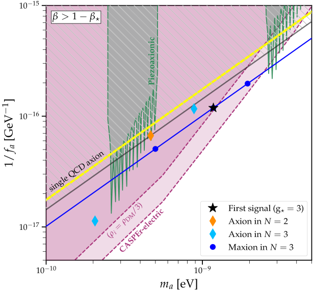
Examples of multi-axion solutions to the strong CP problem are illustrated in Fig. 2. If a experiment detects a signal at the location indicated by the star, and it corresponds to a pure QCD axion solution, it is predicted that
-
•
No signal should be found inside all the dashed area –delimitated by a grey line, including in particular the standard -yellow- QCD line.
-
•
A second axion signal should be found in the undashed area. For the and the toy model above, its location is marked in the figure by an orange diamond.
The first point stems from the sum rule in Eq. (13), and in fact it will hold whatever the total number of axion eigenstates, see next section. There, we will generalize that sum rule to an arbitrary number of axion eigenstates for generic PQ-invariant potentials.
In addition, Fig. 1 indicates that, for the eigenstate closest the the standard QCD band, the point of largest departure corresponds to (case not illustrated in Fig. 2); this fact will turn out to extend to arbitrary mixing potentials 333In the particular example above, the value which allows maximal departure of the eigenstate closest to the standard QCD band is . Using the same simple potential, but for different and , that maximal deviation is given by ..
The results above for the QCD band apply directly to experiments which are independent of the axion UV complete models, such as CASPEr-electric JacksonKimball:2017elr or future experiments based on the piezoaxionic effect Arvanitaki:2021wjk . It is easy to prove, though, that the couplings to photons and nucleons get analogously displaced under some simplifying assumptions, see Section III.2 for this analysis in the generic axion scenario.
III Multiple QCD axion fields
It will be shown next that whenever the axion field (or field combination) that couples to mixes with other scalar singlets via a PQ-invariant potential, it will lead in all generality to axion eigenstates, i.e. distinct massive pseudoscalars, each of them coupling to in a very specific way.
Let us first formulate the general case of a system of scalar fields which couple to the QCD topological term through one arbitrary linear combination, and are in addition subject to an extra scalar potential which mixes them,
| (14) |
where, without loss of generality, the decay constants have been redefined to absorb any coefficient in the coupling to gluons. Without the extra potential, the system would have exhibited independent global U(1) symmetries at the classical level, with one combination of the GBs becoming the standard massive QCD axion. The mixing potential reduces the symmetry. To be precise, note that neither the number of fields that couple to nor the dimension of the mixing potential needs to coincide with the number of scalars in Nature which mix, but the results below are independent of it, as shown in the basis of Eq. (19).
The condition to solve the strong CP problem in the presence of the potential is simply that the latter must exhibit a symmetry, i.e. solely broken by QCD. Imposing this true PQ symmetry ensures that the minimum of the complete potential corresponds to the CP conserving point, , and it will have important consequences on the properties of the different axions. From now on we will assume that all axion fields are already redefined and expanded around their minimum and thus we will drop the -term.
It is instructive to consider the complete scalar mass matrix which stems from Eq. (14). At energies below the QCD confinement scale, the gluonic coupling induces a non-zero potential444The leading order QCD axion potential DiVecchia:1980yfw ; Leutwyler:1992yt ; diCortona:2015ldu reads , where . which corresponds to the following mass term,
| (15) |
where the QCD topological susceptibility was defined on the right-hand side (RHS) of Eq. (1). The complete mass matrix can then be defined as
| (16) |
where
has rank and encodes the QCD contribution to the masses of the axion eigenstates, while stems from the extra potential.
If the system has a PQ symmetry, the determinant of the complete mass matrix needs to vanish in the limit where the QCD topological susceptibility goes to zero, which in turn implies that the determinant of vanishes555In order for the result to apply both ways, one needs to add on the RHS the condition that the eigenvector of with vanishing eigenvalue, (see App. B), has a non-zero projection to the linear combination that couples to gluons, i.e. . ,
| (17) |
A rotated basis. The problem can be equivalently formulated rotating to a field basis in which the combination of fields coupled to is redefined as a single field ,
| (18) |
and as a consequence mixes with the remaining fields via the (rotated) external potential ,
| (19) |
The relation of the scale to the set in Eq. (18) follows from field normalization. In this perspective, the field coupling to is allowed to mix with other singlet scalars in Nature through a PQ-invariant potential. This is the generalization of the rotation performed earlier for between Eqs. (4) and Eqs. (5). The rotated basis will be preferred further below, as it renders particularly straightforward mathematical demonstrations.
Peccei-Quinn condition
In the rotated basis, the square mass matrix can again be decomposed in two parts, where the part proportional to , , is now diagonal and has only one non-zero element corresponding to ,
| (22) | ||||
| (27) |
in which both and the minor666By minor matrix we mean the submatrix resulting from deleting the first row and column. are matrices, is a -dimensional column vector and is a scalar. The PQ-invariance condition in Eq. (17) reads now,
| (28) |
and applying the Schur complement it follows that
| (29) |
Assuming that all axions become massive777Our result can also be applied if some axions were to be massless. If out of the eigenstates are massless, one can simply block diagonalize those scalars first (which in fact decouple from the QCD sector), and then apply the result to the dimensional matrix. , i.e. , the second factor in Eq. 29 must vanish and applying again the Schur complement to the complete matrix in the rotated basis, in Eq. (22), we obtain in all generality that the necessary condition for a scalar potential to be PQ invariant is
| (30) |
i.e.
| (31) |
plus the mixing condition stated in Footnote 5. For a given mass eigenstate with eigenvalue , let denote the physical strength of its coupling to gluons,
| (32) |
Denoting by the elements of the rotation matrix that diagonalizes (which define the eigenvectors of the system), the projection of onto the unit vector which couples to gluons reads
| (33) |
It then follows that can then be expressed as
| (34) |
while
| (35) |
that is, the physical coupling to gluons of a given axion eigenstate can be seen as the projection of the coupling of into that eigenstate.
III.1 Distance from the standard axion band
The physical, measurable, quantities are and . How much can their value depart from the standard QCD band, defined by Eq. (1)?
The factor of defined in Eq. 2 precisely describes how much the mass-scale relation for an eigenstate deviates from that for the single QCD axion. In light of Eq. (35) the factors can be expressed in the preferred basis as
| (36) |
which in turn implies in terms of :
| (37) |
which shows that is the fraction of a given mass eigenvalue due to QCD, its “axionness”.
A sum rule.
It is fruitful to apply now the eigenvalue-eigenvector identity JacobiDeBQ ; Denton:2019pka (see Eq. 88). In one of its versions it reads
| (38) |
where denotes any Hermitian matrix with eigenvalues and associated eigenvectors , and where denotes the minor matrix formed by removing the row and column of . Applying this identity to the mass matrix in the preferred basis in Eq. 27, , it implies for and that
| (39) |
By comparison with the requirement that the potential has a true PQ symmetry, Eq. 31, the following constraint on the possible values of the factors results:
| (40) |
or equivalently
| (41) |
An alternative derivation of this QCD axion sum rule can be found in App. B, which provides an intuitive understanding of axionness.
This sum rule links the multiple QCD axion signals and allows a direct comprehension of the decoupling limits in which only one single QCD axion is reachable. In order to obtain a different phenomenology with respect to this standard case, at least one scale in the mixing potential is required to be of the order of the QCD induced mass scale, a fact we demonstrate in App. C.
Furthermore, a number of properties of the multiple axion eigenstates follow from our sum rule, as we will rigorously prove next.
-
1.
All -factors are larger or equal than one,
(i.e. ), as a consequence of the positivity of the extra potential. i.e. of being positive semi-definite. For a true PQ symmetry, this implies that the QCD axion line in the parameter space of any of these multiple axions can only be displaced to the right of that of the single axion case, by a factor .
Proof. Combining the expression for the mass eigenvalues in the rotated basis, Eq. (34), with Eq. (81), it results that
(42) since is semi-positive definite888The mass matrix of a system of axions is defined as the second derivative in the minimum of the potential and thus it is semi-positive definite. However, if one splits the mass matrix in two contributions, nothing guarantees that both matrices are still semi-positive definite. We argue, nevertheless, that this is indeed the case for our matrices. Due to the PQ symmetry, has vanishing determinant and thus there are more axions than constraints in the extra potential in order to find the minimum. . It follows that .
-
2.
If a given axion has a factor , the sum rule sets an upper limit on the -factor of any other axion,
(43) or, equivalently
(44) Proof. This follows directly from the inequality
(45) This bound has interesting experimental consequences as we will discuss in Section V.
-
3.
As a particular case of the previous property, if one axion is detected with , then no other axion eigenstate can couple to gluons and thus no other axion signal is to be expected. Conversely, it is enough to detect one axion signal with to imply that at least another axion signal awaits discovery.
-
4.
Maximal distance of the axion closest to standard: Maxions. The maximum value that the smallest of all ’s can take is , the number of physical axions, and it corresponds to the case where all of them are equal,
(46) This follows directly from the sum-rule in Eq. (40), that shows that if any deviates from the point where all are equal, another one has to deviate contrarily following a see-saw pattern. In the scenario in Eq. (46), all the axion signals will appear aligned over just one QCD line parallel to that for the single QCD axion, and displaced to its right by a factor . We will denominate this type of solutions as QCD maxions (maximally deviated QCD axions).
For maxions, the coefficients of the characteristic polynomial of ,
(47) and the analogous ones for the minor , , fulfill the relation
(48) These coefficients can be expressed in all generality in terms of the complete exponential Bell polynomials,
(49) and then the relation in Eq. (48) reads
(50) This constitutes a set of QCD maxion conditions necessary to solve the strong CP problem via maxions. For the particular case in which all decay constants in Eq. (14) are equal, , it follows that and these relations simplify to
(51) A particular relation of interest is that for , which implies the following constraint the sum of all square maxion masses:
(52) Furthermore, for the maxion condition boils down to the PQ constraint on the determinants of a generic potential, Eq. 31. The proof of the relations in Eq. (51) is somewhat lengthy, and we have thus deferred it to App. D.
Interestingly, the maxion conditions are automatically fulfilled by Laguerre polynomials, as explained in Section IV. Mixing matrices in clockwork scenarios Kim:2004rp ; Choi:2014rja ; Kaplan:2015fuy ; Giudice:2016yja , on the contrary, do not in general satisfy these maxion conditions, as shown in App. E.
III.2 Extension to the coupling to photons
It is not completely straightforward to extend the constraints studied above for the axion-gluon coupling to the interactions to photons. The reason is that the axion-photon coupling has a component that depends on the UV axion model through the ratio , where denotes the model-dependent electromagnetic anomaly and the color anomaly.
A simple case is that in which is assumed to be equal for all axion fields in Eq. (14), , . The model-dependent axion-photon interactions read then
| (53) |
which in terms of the preferred rotated basis becomes
| (54) |
i.e. the axion-photon coupling is aligned with the gluonic one, see Eq. (19). This already suggests that the fate of the standard band for the QCD axion-photon coupling will follow a very similar pattern to that determined for the coupling to gluons. The physical coupling to photons will receive as usual a model-independent QCD contribution stemming from the axion--pion mixing. This component can be easily computed by performing an axion-dependent rotation on the quark fields Georgi:1986df ; diCortona:2015ldu ,
| (59) |
where the matrix is chosen so that the tree-level axion-pion mixing is avoided, , where denotes the quark mass matrix. In other words, it is chosen so that the mass matrix for is automatically diagonal. This anomalous rotation modifies the coupling to photons as customary with a shift on of -where is the electric quark charge matrix- leading to diCortona:2015ldu ,
| (60) |
where in the last step next-to-leading corrections in the chiral expansion have been incorporated. Finally, in terms of the mass eigenvalues and physical scale of the eigenstates , the axion-photon interactions, for this universal case, are given by
| (61) |
This implies that the single QCD axion band in the coupling to photons will be shifted by the same factor of that has been determined for the gluon-axion coupling in the previous section,
| (62) |
A sum rule for the coupling to photon of the axion excitations follows (analogous to that for the PQ condition in Eq. (40)),
| (63) |
Two plausible scenarios in which would be universal for all axions -and thus the results above hold directly- are: i) the UV models in which no exotic fermions are electromagnetically charged i.e. , and ii) when the SM is embedded in a Grand Unified Theory (GUT), which can fix Srednicki:1985xd ; Agrawal:2022lsp . In fact, the authors of Ref. Agrawal:2022lsp already noted that, in the presence of multiple axions in a GUT theory, their photon-couplings were always located to the right of the standard axion-photon band. They did not explore the fundamental axion-gluon coupling, though, neither determined the maximal distances nor the general proofs and sum-rules obtained here.
The more general case in which differs for each of the axion fields can be worked out from the results above.
IV Maxion masses
Even though the maxion conditions require the presence of mass scales in the extra potential which are of the same order as the QCD-induced mass, and restrict the shape of the matrices, there are still infinitely many maxion matrices. Indeed, the class of matrices that verify these QCD Maxion conditions generate a -parameter family of matrices with . Fixing all , the number of families reduces to . Consequently, in the latter case all maxion potentials are functions of free parameter(s), plus the overall scale.
In a scenario with 2 axion fields produced with the same decay constant (), the only family of maxions is characterized by the following mass matrix:
| (64) |
where . For , the toy example presented in Sec. II is recovered, while reproduces the example in App. A.
The eigenvalues obtained from this matrix lead to ranging from . In the limiting case in which , corresponding to , the system is not PQ-invariant, as the massless eigenstate has no mixing with ; see Footnote 5. Nonetheless, values of (with ) are possible, corresponding to an almost massless maxion and another one with . This shows that highly hierarchical masses are possible. Assuming a different hierarchy for and , values of can be attained in addition.
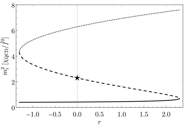
In scenarios with 3 axions, the maxion families are instead characterized by 3 free parameters, assuming equal decay constants for all fields. Identifying with the PQ combination, an illustrative example is given by the mass matrix
| (65) |
with . The eigenvalues sourced by this mass matrix are shown in Fig. 4. If it was furthermore assumed that the extra source of interactions is diagonal in the scalar fields, it would follow that:
| (66) |
In this particular example, the entries of in the preferred basis turn out to be simply the roots of Laguerre polynomials, as explained next.
Laguerre maxions. If the matrix in Eq. 16 is diagonal and all decay constants are equal , one can show that the maxion conditions are automatically fulfilled if the characteristic polynomial of the mass matrix and its minor –in the preferred rotated basis– correspond to the Laguerre polynomials and . We call the solutions produced in this scenario Laguerre maxions. Indeed, one can check that for the zeroes of the -th order Laguerre polynomial , the following identity holds999This can be shown using the expression of in Eq. 90 and the property . ,
| (67) |
ensuring that all physical axions depart from the standard QCD axion line by a factor of . The Laguerre Maxion scenario is particularly predictive since the spread in the values of the QCD axion masses will be fixed and determined by the zeroes of the Laguerre polynomials (see example the cases of in Fig. 4).
V Discussion and outlook
The main experimental impact of our results is that multiple axion signals –instead of a single one– are expected from the generic QCD axion solution to the strong CP problem. The customary solution with a single axion QCD corresponds instead to a certain limit of the general parameter space. These multiple solutions can only be displaced towards the right of the customary QCD axion band.
In case of a positive ALP signal to the right of that band (or even within the single QCD band given its error bars), experiments are encouraged to look for similar signals within their frequency range. In addition, signals widely separated and thus accessed by different experiments are possible. This establishes a beautiful synergy between experiments sensitive to vastly different masses and scales, as the complete reconstruction of the solution to the strong CP problem may require this complementary search.
An illustration of this experimental impact on the parameter space of axion-gluon couplings (which are directly tackled by axion-nEDM experiments) is provided in Fig. 2. Specific and QCD axion solutions are depicted, corresponding to mixing matrices in Eqs. 7 and 66 and a generic 3-axion scenario. A star indicates the putative location of the first signal detected in the axion/ALP parameter space. For it to be linked to a pure axion QCD solution of the strong CP problem, it follows that:
-
•
No other axion signal can be found anywhere in the greyed area (which includes the single QCD axion band). This holds independently of the total number of axion eigenstates .
-
•
For only a second signal should appear exactly in the grey line, so as to saturate the sum rule; an example is indicated by an orange diamond.
-
•
For , two other signals await discovery in the undashed area, see e.g. the clear blue diamonds.
-
•
An maxion solution is also possible in the example chosen, signaled by the dark blue points, as the distance of the star signal to the single QCD axion band is .
We have shown that the same pattern holds for arbitrary , for which we have determined in all generality the condition for an arbitrary scalar potential to be PQ invariant. Furthermore, a precise sum rule for the QCD axion has been found, together with other exact results.
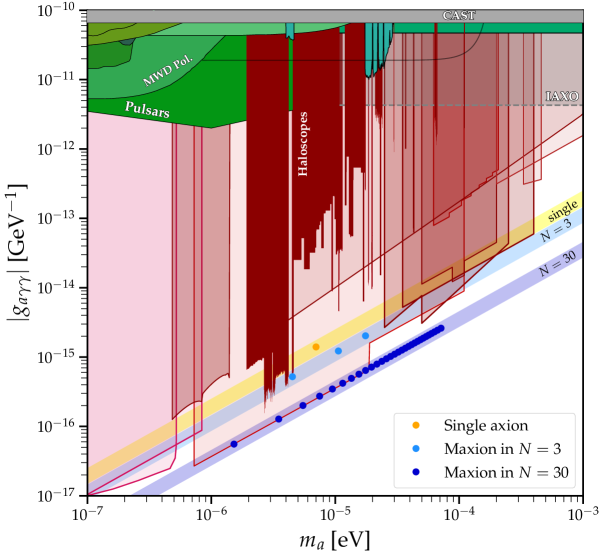
For the axion-photon couplings, we have illustrated the analogous multiple signals and displacements in Fig. 3, assuming universal couplings and focusing on maxion signals: both a and a maxion multiplet are shown, for the mixing provided by the Laguerre matrices described in Section IV. The displacements of axion couplings to elementary fermions will be subject to model-dependences analogous to those of axion-photon couplings, to be further explored elsewhere future .
In practice, for signals close to the standard QCD band the possible displacement of a given signal will be obscured by the incertitude on the width of the band itself. For experiments measuring directly the coupling to gluons, there is a large uncertainty on the theoretical prediction of EDM JacksonKimball:2017elr . For axion-photon searches, the experimental measurements are very precise with uncertainties stemming instead from the UV model dependence, i.e. the different matter content of axion models and different factors. In summary, the smoking gun may turn out to be the multiplicity of signals, as experiments have reached impressive precision on frequencies.
Furthermore, most of the experiments with best reach rely on the assumption that axions account for the dark matter (DM) of the universe. Haloscopes are sensitive to , where denotes the local DM density and a generic axion coupling to the visible world. Uncertainties stem from (which could be largely modified by miniclusters, focusing effects, etc.) and, for the multiple QCD axion under discussion, on how DM is distributed among them. If democratically distributed among the axion eigenstates, the flux of each species would diminish by a factor of and consequently the bounds would be weakened. We have illustrated this weakening of the projected bounds for CASPEr-electric in Fig. 2, for the scenario. Nevertheless, the thermal evolution of the Universe with a multiple QCD axion may lead to very different spectra and evolution scenarios (e.g. Kitajima:2014xla ; Ho:2018qur ; Cyncynates:2021xzw ; Adams:2022pbo ), which deserve a dedicated future study.
The quest to unravel the fundamental symmetries of the visible and dark sectors of the Universe is inspiring. We have proven that the PQ solution to the strong CP problem within pure QCD leads in all generality to multiple axion signals with well delimitated properties. This stems from lifting the requirement that the basis of axion-gluon interactions and the axion mass basis are simultaneously diagonal.
In this perspective, the usual single QCD axion is just one particular case of the landscape of solutions, corresponding to zero mixing. The results open novel experimental territory
and
blur the distinction between the search for the QCD axion and that for ALPs
in a huge region of the parameter space.
Acknowledgments.—We are indebted to Daniel Alvarez-Gavela for useful discussions and input. We also thank Aneesh Manohar and Benjamin Grinstein for interesting discussions. This project has received funding /support from the European Union’s Horizon 2020 research and innovation programme under the Marie Sklodowska -Curie grant agreement No 860881-HIDDeN, and under the Marie Sklodowska-Curie Staff Exchange grant agreement No 101086085-ASYMMETRY. The work of M. R. is supported by the Marie Sklodowska -Curie grant agreement No 860881-HIDDeN. The work of P.Q. is supported in part by the U.S. Department of Energy Grant No. DE-SC0009919. B. G. acknowledge as well partial financial support from the Spanish Research Agency (Agencia Estatal de Investigación) through the grant IFT Centro de Excelencia Severo Ochoa No CEX2020-001007-S and through the grant PID2019-108892RB-I00 funded by MCIN/AEI/ 10.13039/501100011033. B.G. thanks very much the Particle Physics group of the University of California San Diego, where part of this work was carried out. Likewise, P. Q. thanks the Galileo-Galilei Institute for theoretical Physics in Florence (GGI) for their warm hospitality, where part of this work was carried out. We are also thankful to Anna Lewis for helping to improve the writing of the manuscript.
Appendix A UV completion
We consider a double version of the KSVZ model Kim:1979if ; Shifman:1979if , with two vector-like fermions and two singlet complex scalars , i.e.
| (68) |
In the absence of , the Lagrangian is invariant under two independent global (and QCD anomalous) axial symmetries. If the potential breaks both spontaneously, the fields can be decomposed in terms of two radial and two angular modes,
| (69) |
Let us assume for simplicity . The corresponding eigenstates are then and . The first plays the role of the canonical QCD axion, with , while the second is massless and decouples from the QCD sector.
Nevertheless, the potential may mix both fields, breaking explicitly the two global symmetries down to just one PQ symmetry. A simple example is given by
| (70) |
which leads at low energies to an effective potential which, expanded to second order, reads:
| (71) |
Defining and considering the preferred basis of Eq. (27), the corresponding mass matrix is
| (72) |
which indeed satisfies the condition for PQ invariant potentials in Eq. 30, with . The system thus reabsorbs at the minimum, solving the strong CP problem.
Among the family of solutions in Eq. (72), it is possible to find maxion ones. Indeed, the maxion condition in Eq. (52) is satisfied in this example for : two maxions are then obtained with .
Note that many other explicit potentials can break explicitly the two symmetries to one symmetry. For instance, would lead precisely to the effective potential in the toy model of Section II.
Appendix B A physical interpretation of the sum rule
In Section III.1 we provided a rather mathematical proof of the sum rule. In order to obtain a more physical intuition for the meaning of the axionness, , and its constraint, we provide here an alternative derivation. The main idea is to impose that the modification of the Lagrangian under a PQ transformation coincides in any starting basis and in the mass basis. This “PQ matching” constrains the possible values of the couplings to gluons and masses of the axion mass eigenstates leading to our sum rule, .
On top of the mass eigenstates , there are two linear combinations of particular importance for the QCD axion system. One of them is the combination that couples to the topological term, , and the other is the one that transforms under the PQ symmetry, . The latter is the combination whose shift is only broken by the QCD anomaly (an equivalent definition is that it corresponds to the eigenvector of with vanishing eigenvalue). We will now show how the axionness of an axion will depend on the projections of a given mass eigenstate onto both of these linear combinations, and .
Let us consider a basis where the mass matrix stemming from the extra potential is diagonal, for . Since the only term that breaks is the term, the extra potential does not contain the field,
(Note that , as defined above, does not need to coincide with the vacuum expectation value of the PQ scalar.)
The mass Lagrangian of the axion system reads,
| (73) |
which under a shift transforms as101010Recall that, by definition, the relevant projections take the following values, and .
Now let us consider the diagonalized mass Lagrangian,
| (74) |
and perform the same transformation:
| (75) | ||||
| (76) | ||||
By imposing the “PQ matching” order by order, we find:
| (77) |
and since , we conclude that
| (78) |
Finally, we reproduce our relation by noting that
that is,
| (79) |
This shows that for an axion mass eigenstate to coincide with the traditional single QCD axion, , the overlap with both and needs to be maximal. Conversely, for a given physical axion to decouple from the sum rule, it is necessary to either have a vanishing projection on the anomalous axion linear combination, , or on the combination implementing the PQ symmetry, . Indeed, it is these two vanishing projections that explain the decoupling of one axion from the sum rule in the example of Section II, in the limits and .
Besides proving the sum rule in Eq. (41) without appealing to the eigenvalue-eigenvector theorem, this derivation directly suggests further relations such as
| (80) |
which may have a more limited phenomenological impact as compared to the previous sum rule, though, because we do not have direct experimental access to . In an eventual multi-axion detection, it could help to reconstruct the whole axion system.
Appendix C Decoupling from the sum rule and mass scales in the extra potential
As we explicitly derived for the toy model in Section II, in the limits where the extra potential is either much smaller or much larger than the QCD contribution, one of the axions decouples from the sum rule. Two pertinent questions arise: how does this behaviour generalize for arbitrary ? Is the contribution from the extra potential required to be of the same order of magnitude as the QCD contribution, in order for all axions to play a relevant role in the sum rule?
Let us consider the basis where the extra mass contribution is diagonal , which corresponds to the states . This is the same basis used in the demonstration in App. B.
Using Appendix B, the -factors can be expressed as
| (81) |
For , one of the mass eigenstates of the full matrix corresponds to , with mass , and it is orthogonal to all the other . Thus, its axionness reads
| (82) |
showing that this state effectively decouples from the sum rule.
In the opposite limit, , or equivalently , one can show that the linear combination,
| (83) |
corresponds to a mass eigenstate of the full matrix with eigenvalue . Therefore,
| (84) |
showing that this state also decouples from the sum rule.
Overall, we have demonstrated that whenever one eigenvalue of , , is either much larger or much smaller than the QCD induced mass scale, , one axion eigenstate decouples from the sum rule and the phenomenology is well described by the axion system.
This statement depends however on the experimental precision. For example, the matrix
| (85) |
with , generates a multiple axion system with . Measuring and with sufficiently high precision could allow us to infer the existence of the third axion (or more) even though .
Appendix D Proof of the QCD maxion conditions
We will show that the necessary and sufficient condition to generate QCD maxions is
| (86) |
determining the characteristic polynomials of and the minor ,
| (87) |
In order to prove this result, we will make use of the eigenvector-eigenvalue identity JacobiDeBQ ; Denton:2019pka stated below.
Theorem. If is an hermitian matrix with eigenvalues and , then the component of a unit eigenvector associated to is related to the eigenvalues of the minor , obtained by removing the row and column of A, by the formula
| (88) |
We will start by proving that implies Eq. 86. Let us first rewrite the -factors in terms of the characteristic polynomials defined above,
| (89) |
Since is a zero of , it follows that and thus the -factor can be expressed in terms of the derivative of the characteristic polynomial evaluated in ,
| (90) |
Differentiating the characteristic polynomial in Eq. 87 and assuming the condition we find:
| (91) | |||
| (92) |
where is the Vandermonde matrix of dimension , whose determinant is
| (93) |
Provided none of the eigenvalues are degenerate, , proving the claim.
Appendix E Comparison with clockwork scenario
In general, clockwork matrices Kim:2004rp ; Choi:2014rja ; Kaplan:2015fuy ; Giudice:2016yja do not generate maxions (one exception being the model comprising only 2 scalars). The reason being that the next neighbor interactions of clockwork scenarios are engineered to generate exponentially small mixings whereas the maxion solutions require sizable mixings. To see a concrete example, we focus on a scenario with three scalars, where the typical clockwork mass matrix (including the QCD contribution) reads:
| (94) |
with and assuming that only one field in the 3rd-site develops couplings to gluons.
One can easily check that the PQ condition is satisfied by this matrix, as . To prove that this model does not generate maxions, it suffices to show that the remaining two maxions conditions spanned by Eq. 86 cannot be satisfied for the same . Indeed,
| (95) | ||||
| (96) |
References
- (1) R. D. Peccei and H. R. Quinn, “CP Conservation in the Presence of Instantons,” Phys. Rev. Lett. 38 (1977) 1440–1443.
- (2) R. D. Peccei and H. R. Quinn, “Constraints Imposed by CP Conservation in the Presence of Instantons,” Phys. Rev. D 16 (1977) 1791–1797.
- (3) S. Weinberg, “A New Light Boson?,” Phys. Rev. Lett. 40 (1978) 223–226.
- (4) F. Wilczek, “Problem of Strong and Invariance in the Presence of Instantons,” Phys. Rev. Lett. 40 (1978) 279–282.
- (5) K. R. Dienes, E. Dudas, and T. Gherghetta, “Invisible axions and large radius compactifications,” Phys. Rev. D 62 (2000) 105023, arXiv:hep-ph/9912455.
- (6) G. B. Gelmini and M. Roncadelli, “Left-Handed Neutrino Mass Scale and Spontaneously Broken Lepton Number,” Phys. Lett. B 99 (1981) 411–415.
- (7) A. Davidson and K. C. Wali, “MINIMAL FLAVOR UNIFICATION VIA MULTIGENERATIONAL PECCEI-QUINN SYMMETRY,” Phys. Rev. Lett. 48 (1982) 11.
- (8) F. Wilczek, “Axions and Family Symmetry Breaking,” Phys. Rev. Lett. 49 (1982) 1549–1552.
- (9) P. Svrcek and E. Witten, “Axions In String Theory,” JHEP 06 (2006) 051, arXiv:hep-th/0605206.
- (10) A. Arvanitaki, S. Dimopoulos, S. Dubovsky, N. Kaloper, and J. March-Russell, “String Axiverse,” Phys. Rev. D 81 (2010) 123530, arXiv:0905.4720 [hep-th].
- (11) M. Cicoli, “Axion-like Particles from String Compactifications,” in 9th Patras Workshop on Axions, WIMPs and WISPs, pp. 235–242. 2013. arXiv:1309.6988 [hep-th].
- (12) S. Alexander, H. Gilmer, T. Manton, and E. McDonough, “The -axion and -axiverse of dark QCD,” arXiv:2304.11176 [hep-ph].
- (13) J. Preskill, M. B. Wise, and F. Wilczek, “Cosmology of the Invisible Axion,” Phys. Lett. B 120 (1983) 127–132.
- (14) L. F. Abbott and P. Sikivie, “A Cosmological Bound on the Invisible Axion,” Phys. Lett. B 120 (1983) 133–136.
- (15) M. Dine and W. Fischler, “The Not So Harmless Axion,” Phys. Lett. B 120 (1983) 137–141.
- (16) V. A. Rubakov, “Grand unification and heavy axion,” JETP Lett. 65 (1997) 621–624, arXiv:hep-ph/9703409.
- (17) Z. Berezhiani, L. Gianfagna, and M. Giannotti, “Strong CP problem and mirror world: The Weinberg-Wilczek axion revisited,” Phys. Lett. B 500 (2001) 286–296, arXiv:hep-ph/0009290.
- (18) L. Gianfagna, M. Giannotti, and F. Nesti, “Mirror world, supersymmetric axion and gamma ray bursts,” JHEP 10 (2004) 044, arXiv:hep-ph/0409185.
- (19) S. D. H. Hsu and F. Sannino, “New solutions to the strong CP problem,” Phys. Lett. B 605 (2005) 369–375, arXiv:hep-ph/0408319.
- (20) A. Hook, “Anomalous solutions to the strong CP problem,” Phys. Rev. Lett. 114 no. 14, (2015) 141801, arXiv:1411.3325 [hep-ph].
- (21) H. Fukuda, K. Harigaya, M. Ibe, and T. T. Yanagida, “Model of visible QCD axion,” Phys. Rev. D 92 no. 1, (2015) 015021, arXiv:1504.06084 [hep-ph].
- (22) C.-W. Chiang, H. Fukuda, M. Ibe, and T. T. Yanagida, “750 GeV diphoton resonance in a visible heavy QCD axion model,” Phys. Rev. D 93 no. 9, (2016) 095016, arXiv:1602.07909 [hep-ph].
- (23) S. Dimopoulos, A. Hook, J. Huang, and G. Marques-Tavares, “A collider observable QCD axion,” JHEP 11 (2016) 052, arXiv:1606.03097 [hep-ph].
- (24) T. Gherghetta, N. Nagata, and M. Shifman, “A Visible QCD Axion from an Enlarged Color Group,” Phys. Rev. D 93 no. 11, (2016) 115010, arXiv:1604.01127 [hep-ph].
- (25) A. Kobakhidze, “Heavy axion in asymptotically safe QCD,” arXiv:1607.06552 [hep-ph].
- (26) P. Agrawal and K. Howe, “Factoring the Strong CP Problem,” JHEP 12 (2018) 029, arXiv:1710.04213 [hep-ph].
- (27) P. Agrawal and K. Howe, “A Flavorful Factoring of the Strong CP Problem,” JHEP 12 (2018) 035, arXiv:1712.05803 [hep-ph].
- (28) M. K. Gaillard, M. B. Gavela, R. Houtz, P. Quilez, and R. Del Rey, “Color unified dynamical axion,” Eur. Phys. J. C 78 no. 11, (2018) 972, arXiv:1805.06465 [hep-ph].
- (29) A. Hook, S. Kumar, Z. Liu, and R. Sundrum, “High Quality QCD Axion and the LHC,” Phys. Rev. Lett. 124 no. 22, (2020) 221801, arXiv:1911.12364 [hep-ph].
- (30) T. Gherghetta and M. D. Nguyen, “A Composite Higgs with a Heavy Composite Axion,” JHEP 12 (2020) 094, arXiv:2007.10875 [hep-ph].
- (31) C. Csáki, M. Ruhdorfer, and Y. Shirman, “UV Sensitivity of the Axion Mass from Instantons in Partially Broken Gauge Groups,” JHEP 04 (2020) 031, arXiv:1912.02197 [hep-ph].
- (32) A. Kivel, J. Laux, and F. Yu, “Supersizing axions with small size instantons,” JHEP 11 (2022) 088, arXiv:2207.08740 [hep-ph].
- (33) A. Hook, “Solving the Hierarchy Problem Discretely,” Phys. Rev. Lett. 120 no. 26, (2018) 261802, arXiv:1802.10093 [hep-ph].
- (34) L. Di Luzio, B. Gavela, P. Quilez, and A. Ringwald, “An even lighter QCD axion,” JHEP 05 (2021) 184, arXiv:2102.00012 [hep-ph].
- (35) L. Di Luzio, B. Gavela, P. Quilez, and A. Ringwald, “Dark matter from an even lighter QCD axion: trapped misalignment,” JCAP 10 (2021) 001, arXiv:2102.01082 [hep-ph].
- (36) D. Budker, P. W. Graham, M. Ledbetter, S. Rajendran, and A. Sushkov, “Proposal for a Cosmic Axion Spin Precession Experiment (CASPEr),” Phys. Rev. X 4 no. 2, (2014) 021030, arXiv:1306.6089 [hep-ph].
- (37) D. F. Jackson Kimball et al., “Overview of the Cosmic Axion Spin Precession Experiment (CASPEr),” Springer Proc. Phys. 245 (2020) 105–121, arXiv:1711.08999 [physics.ins-det].
- (38) J. E. Kim, H. P. Nilles, and M. Peloso, “Completing natural inflation,” JCAP 01 (2005) 005, arXiv:hep-ph/0409138.
- (39) K. Choi, H. Kim, and S. Yun, “Natural inflation with multiple sub-Planckian axions,” Phys. Rev. D 90 (2014) 023545, arXiv:1404.6209 [hep-th].
- (40) D. E. Kaplan and R. Rattazzi, “Large field excursions and approximate discrete symmetries from a clockwork axion,” Phys. Rev. D 93 no. 8, (2016) 085007, arXiv:1511.01827 [hep-ph].
- (41) G. F. Giudice and M. McCullough, “A Clockwork Theory,” JHEP 02 (2017) 036, arXiv:1610.07962 [hep-ph].
- (42) L. Di Luzio, F. Mescia, E. Nardi, P. Panci, and R. Ziegler, “Astrophobic Axions,” Phys. Rev. Lett. 120 no. 26, (2018) 261803, arXiv:1712.04940 [hep-ph].
- (43) Z. Chen, A. Kobakhidze, C. A. J. O’Hare, Z. S. C. Picker, and G. Pierobon, “Phenomenology of the companion-axion model: photon couplings,” Eur. Phys. J. C 82 no. 10, (2022) 940, arXiv:2109.12920 [hep-ph].
- (44) P. Agrawal, M. Nee, and M. Reig, “Axion couplings in grand unified theories,” JHEP 10 (2022) 141, arXiv:2206.07053 [hep-ph].
- (45) K. Fraser and M. Reece, “Axion Periodicity and Coupling Quantization in the Presence of Mixing,” JHEP 05 (2020) 066, arXiv:1910.11349 [hep-ph].
- (46) L. Darmé, L. Di Luzio, M. Giannotti, and E. Nardi, “Selective enhancement of the QCD axion couplings,” Phys. Rev. D 103 no. 1, (2021) 015034, arXiv:2010.15846 [hep-ph].
- (47) C. G. J. Jacobi, “De binis quibuslibet functionibus homogeneis secundi ordinis…,” Journal für die reine und angewandte Mathematik (Crelles Journal) 1834 1 – 69.
- (48) P. B. Denton, S. J. Parke, T. Tao, and X. Zhang, “Eigenvectors from Eigenvalues: a survey of a basic identity in linear algebra,” Bull. Am. Math. Soc. 59 no. 1, (2022) 31–58, arXiv:1908.03795 [math.RA].
- (49) A. Arvanitaki, A. Madden, and K. Van Tilburg, “The Piezoaxionic Effect,” arXiv:2112.11466 [hep-ph].
- (50) C. O’Hare, “cajohare/axionlimits: Axionlimits.” https://cajohare.github.io/AxionLimits/, July, 2020.
- (51) P. Di Vecchia and G. Veneziano, “Chiral Dynamics in the Large n Limit,” Nucl. Phys. B 171 (1980) 253–272.
- (52) H. Leutwyler and A. V. Smilga, “Spectrum of Dirac operator and role of winding number in QCD,” Phys. Rev. D 46 (1992) 5607–5632.
- (53) G. Grilli di Cortona, E. Hardy, J. Pardo Vega, and G. Villadoro, “The QCD axion, precisely,” JHEP 01 (2016) 034, arXiv:1511.02867 [hep-ph].
- (54) H. Georgi, D. B. Kaplan, and L. Randall, “Manifesting the Invisible Axion at Low-energies,” Phys. Lett. B 169 (1986) 73–78.
- (55) M. Srednicki, “Axion Couplings to Matter. 1. CP Conserving Parts,” Nucl. Phys. B 260 (1985) 689–700.
- (56) B. Gavela, P. Quilez, M. Ramos (work on progress).
- (57) N. Kitajima and F. Takahashi, “Resonant conversions of QCD axions into hidden axions and suppressed isocurvature perturbations,” JCAP 01 (2015) 032, arXiv:1411.2011 [hep-ph].
- (58) S.-Y. Ho, K. Saikawa, and F. Takahashi, “Enhanced photon coupling of ALP dark matter adiabatically converted from the QCD axion,” JCAP 10 (2018) 042, arXiv:1806.09551 [hep-ph].
- (59) D. Cyncynates, T. Giurgica-Tiron, O. Simon, and J. O. Thompson, “Resonant nonlinear pairs in the axiverse and their late-time direct and astrophysical signatures,” Phys. Rev. D 105 no. 5, (2022) 055005, arXiv:2109.09755 [hep-ph].
- (60) C. B. Adams et al., “Axion Dark Matter,” in Snowmass 2021. 3, 2022. arXiv:2203.14923 [hep-ex].
- (61) J. E. Kim, “Weak Interaction Singlet and Strong CP Invariance,” Phys. Rev. Lett. 43 (1979) 103.
- (62) M. A. Shifman, A. I. Vainshtein, and V. I. Zakharov, “Can Confinement Ensure Natural CP Invariance of Strong Interactions?,” Nucl. Phys. B 166 (1980) 493–506.