The QED four – photon amplitudes off-shell: part 1

Naser Ahmadiniaz n.ahmadiniaz@hzdr.de Cristhiam Lopez-Arcos cmlopeza@unal.edu.co Misha A. Lopez-Lopez misha.lopez@umich.mx Christian Schubert christianschubert137@gmail.com Helmholtz-Zentrum Dresden-Rossendorf, Bautzner Landstraße 400, 01328 Dresden, Germany Center for Relativistic Laser Science, Institute for Basic Science, 61005 Gwangju, Korea Escuela de Matemáticas, Universidad Nacional de Colombia Sede Medellín, Carrera 65

\#

59A–110, Medellín, Colombia Instituto de Física y Matemáticas Universidad Michoacana de San Nicolás de Hidalgo Edificio C-3, Apdo. Postal 2-82 C.P. 58040, Morelia, Michoacán, México

Abstract

The present paper is the first in a series of four where we use the worldline formalism to obtain the QED four-photon amplitude completely off-shell. We present the result explicitly in terms of hypergeometric functions, and derivatives thereof, for both scalar and spinor QED. The formalism allows us to unify the scalar and spinor loop calculations, avoiding the usual breaking up of the amplitude into Feynman diagrams, and to achieve manifest transversality at the integrand level as well as UV finiteness term by term by an optimized version of the integration-by-parts procedure originally introduced by Bern and Kosower for gluon amplitudes. The full permutation symmetry is maintained throughout, and the amplitudes get projected naturally into the basis of five tensors introduced by Costantini et al. in 1971. Since in many applications of the “four-photon box” some of the photons can be taken in the low-energy limit, and the formalism makes it easy to integrate out any such leg, apart from the case of general kinematics (part 4) we also treat the special cases of one (part 3) or two (part 2) photons taken at low energy. In this first part of the series, we summarize the application of the worldline formalism to the N-photon amplitudes and its relation to Feynman diagrams, derive the optimized tensor-decomposed integrands of the four-photon amplitudes in scalar and spinor QED, and outline the computational strategy to be followed in parts 2 to 4. We also give an overview of the applications of the four-photon amplitudes, with an emphasis on processes that involve some off-shell photons. The case where all photons are taken at low energy (the “Euler-Heisenberg approximation”) is simple enough to be doable for arbitrary photon numbers, and we include it here for completeness.

^†^†journal: .

1 Introduction: Photon amplitudes in QED

Classical electrodynamics is described by Maxwell’s equations, which are linear in both sources and fields. Non-linear corrections to Maxwell’s theory appear as purely quantum effects that violate the superposition principle and, among other things, give rise to the possible polarization of the vacuum.

Dirac’s prediction of the positron [1, 2] led to the possibility of creation and annihilation of virtual particles, non-linear effects that have as a particular consequence the possibility of the light-by-light (LBL) scattering process. This effect was first studied in 1936 by W. Heisenberg and H. Euler [3] where they, still using Dirac’s hole theory, obtained their famous closed-form expression one-loop effective Lagrangian for spinor particles in a constant background field. In modern conventions, the Euler-Heisenberg (EH) Lagrangian is given by

\mathcal{L}_{\rm EH}=-\frac{1}{8\pi^{2}}\int_{0}^{\infty}\frac{dT}{T^{3}}{\rm e}^{-m^{2}T}\left\{\frac{(eaT)(ebT)}{\tan(eaT)\rm tanh({\it ebT})}-\frac{2}{3}(eT)^{2}\mathcal{F}-1\right\},

(1.1)

with

a=\left(\sqrt{\mathcal{F}^{2}+\mathcal{G}^{2}}-\mathcal{F}\right)^{1/2}~{},~{}~{}~{}~{}~{}~{}~{}b=\left(\sqrt{\mathcal{F}^{2}+\mathcal{G}^{2}}+\mathcal{F}\right)^{1/2},

(1.2)

with the two invariants of the Maxwell field

	$\displaystyle-2\mathcal{F}=-\frac{1}{2}F_{\mu\nu}F^{\mu\nu}$	$\displaystyle=$	$\displaystyle\vec{E}^{2}-\vec{B}^{2}\,,$
	$\displaystyle-\mathcal{G}=-\frac{1}{4}F_{\mu\nu}\tilde{F}^{\mu\nu}$	$\displaystyle=$	$\displaystyle\vec{E}\cdot\vec{B}\,.$

Shortly later, an analogous expression was found for the scalar QED by Weisskopf [4],

\mathcal{L}_{\rm W}=\frac{1}{16\pi^{2}}\int_{0}^{\infty}\frac{dT}{T^{3}}{\rm e}^{-m^{2}T}\left\{\frac{(eaT)(ebT)}{\sin(eaT)\sinh({\it ebT})}+\frac{1}{6}(eT)^{2}\mathcal{F}-1\right\}.

(1.4)

See [5] for a comprehensive review of the effective Lagrangians (1.1) and (1.4), their applications and generalizations. They are non-perturbative in the field, but have a perturbative expansion in powers of the field (“weak-field expansion”). For the spinor QED case, it corresponds to the Feynman diagrams shown in Fig. 1, where the “cross” denotes the interaction with the field. For scalar QED, there are additional diagrams involving the quartic seagull vertex. When specialized to a multi-photon background, these diagrams (now without the crosses) represent the $N$ -photon amplitudes in the low-energy limit, where all the photon energies are small compared to the electron mass.

Refer to caption — Figure 1: Diagrammatic perturbative expansion of the EH effective action, eq. (1.1). The first and second diagrams are show in parenthesis because they get removed by on-shell renormalization.

The order $e^{4}$ (or $\alpha^{2}$ , $\alpha=\frac{e^{2}}{4\pi}$ being the fine structure constant) of this expansion gives the lowest-order photon-photon scattering diagram, or rather diagrams, since one has to sum over the six possible orderings of the four photons (see below, Fig. 12).

In this low-energy limit, the first calculation of the cross section for photon-photon scattering was done by H. Euler and B. Kockel [6, 7]. Shortly later, this was followed by a calculation of the opposite high-energy limit by A. Akhiezer et al. [8, 9].

In the low-energy limit, it is a textbook exercise to obtain an explicit expression for the four-photon amplitude (for spinor QED) from the effective Lagrangian (1.1) (see, e.g., [10, 11]). Introducing the field strength tensor $f_{i}^{\mu\nu}$ for photon $i$ ,

f_{i}^{\mu\nu}\equiv k_{i}^{\mu}\varepsilon_{i}^{\nu}-\varepsilon_{i}^{\mu}k_{i}^{\nu},

(1.5)

related to the field strength tensor $F^{\mu\nu}$ by

F^{\mu\nu}=if_{\rm tot}^{\mu\nu}\equiv i\sum_{i=1}^{N}f_{i}^{\mu\nu},

(1.6)

the spinor amplitude for low energy photons can be written as

	$\displaystyle{\cal M}$	$\displaystyle=$	$\displaystyle\frac{2\alpha^{2}}{45m^{4}}\Big{\{}14\left[{\rm tr}(f_{1}f_{2}f_{3}f_{4})+{\rm tr}(f_{1}f_{2}f_{4}f_{3})+{\rm tr}(f_{1}f_{3}f_{2}f_{4})\right]$		(1.7)
			$\displaystyle-5\left[{\rm tr}(f_{1}f_{2}){\rm tr}(f_{3}f_{4})+{\rm tr}(f_{1}f_{3}){\rm tr}(f_{2}f_{4})+{\rm tr}(f_{1}f_{4}){\rm tr}(f_{2}f_{3})\right]\Big{\}}\,.$		(1.7)

Then, in the center of mass frame and after some algebra one can obtain the cross section

\sigma=\frac{973}{10125}\left(\frac{\alpha^{4}}{\pi m^{2}}\right)\left(\frac{\omega}{m}\right)^{6}~{}~{}~{}~{}~{}{\rm for}~{}~{}~{}~{}~{}~{}\frac{\omega}{m}\ll 1.

(1.8)

Similarly, one can use the Weisskopf Lagrangian (1.4) to compute the same cross section for scalar QED.

On the other hand, computing the cross section for LBL scattering in the high energy limit is a much harder task. Even so, Akhiezer et al. were able to obtain the following formula for the differential cross section in this limit [8, 9]

\sigma=\frac{e^{8}}{2\pi\omega^{2}}~{}C~{}~{}~{}~{}~{}{\rm for}~{}~{}~{}~{}~{}~{}\frac{\omega}{m}\gg 1,~{}~{}~{}m=0\,,

(1.9)

but with a numerical constant $C$ that they were unable to calculate. They also showed that $\sigma$ has a maximum in the region $\omega\sim m$ . A numerical value for the constant $C$ was given in [12] as $\frac{C}{2\pi}=4.7$ , and an analytical one finally in [13]

C=\frac{108}{5}+\frac{13}{2}\pi^{2}-8\pi^{2}\zeta(3)+\frac{148}{225}\pi^{4}-24\zeta(5).

(1.10)

For a comprehensive review of the early history of these calculations see [14].

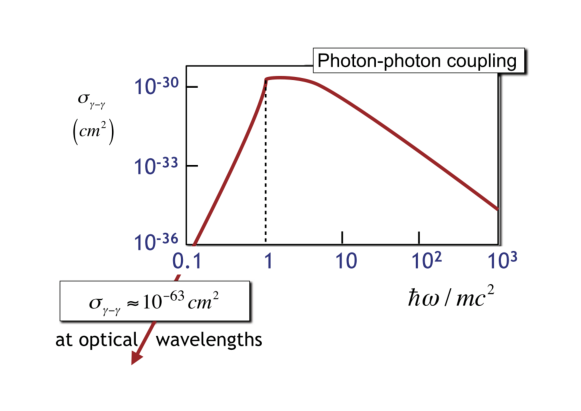
The first treatment of the photon-photon scattering amplitude for arbitrary on-shell kinematics was done by Karplus and Neuman in 1950 [15, 16]. They analyzed the tensor structure of the four-photon amplitude, showed its finiteness and gauge invariance, and managed to express it by three-parameter integrals of rational functions of the external momenta. In the mid-sixties De Tollis [17, 18] recalculated the amplitude using dispersion relation techniques, which led to a more compact form of the result. Using the results of either Karplus and Neuman or De Tollis, it is possible to compute and plot the cross section (see Fig. 2), and to compute the constant $C$ in (1.10).

From a computational point of view, this essentially settled the on-shell case. Further work on on-shell photonic amplitudes focused on higher-point and higher-loop amplitudes, and generalization to SUSY QED and electroweak contributions. The six photon amplitude was computed in massless scalar QED [20] and the $N$ -photon amplitudes in the low-energy limit for both scalar and spinor QED [21, 22]. For two-loop corrections to LBL scattering in spinor QED see [23], in supersymmetric QED [24]. Photon-photon scattering via a W-boson loop has been studied in [25, 26].

However, eventually the need was felt to calculate the four-photon amplitudes also with some legs off-shell. Photons emitted or absorbed by an external field in general can not be assumed to obey on-shell conditions. An important example is Delbrück scattering, the elastic scattering of a photon by a nuclear electromagnetic field, where the scattered photon can be taken real but the interaction with the field is described by virtual photons (see the left-hand diagram of Fig. 8 below). This process, and similar ones involving interactions with the Coulomb field, prompted V. Costantini et al. in 1971 [27] (see also [28]) to study the four-photon amplitude with two photons on-shell and two off-shell. In the same work, they performed a general analysis of the tensor structure of the four-photon amplitude, which from the beginning is written in terms of $138$ tensors. Using the permutation symmetry and the Ward identity they were able to reduce this number to a basis of five invariant tensors.

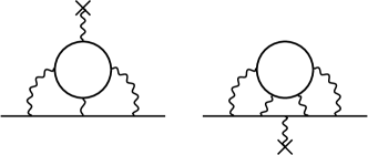
Although their work dates back half a century, to the best of our knowledge no further progress has been made towards the actual calculation of the fully off-shell case. In our opinion, this state of affairs is quite unsatisfactory considering the fact that multiloop QED calculations have long ago reached the stage where the LBL scattering diagram appears fully off-shell, for example, as a subdiagram in the calculation of the three- and higher loop anomalous magnetic momentum, see Fig. 3.

Thus the present series of four papers is devoted to the study of the fully off-shell four-photon amplitudes in scalar and spinor QED. While this would be feasible using standard techniques, here we will take advantage of the recently developed “string-inspired worldline formalism” that has been shown to have significant technical advantages particularly in the computation of photonic processes.

Methods for amplitude calculations inspired by string theory emerged in the seventies with the work of J.L. Gervais and A. Neveu [29] where they observed some simplification of quantum field theory computations in the limit of infinite string tension. In the nineties, it led Z. Bern and D. Kosower to start a systematic investigation of the field theory limit at tree- and loop-level using various string models [30]. In particular, they established a new set of rules for the construction of the one-loop $N$ -gluon amplitudes in QCD which bypasses many steps of the ordinary quantum field theory computation based on Feynman rules. The relation of these rules to the Feynman ones was clarified in [31]. Later, M. Strassler [32] was able to rederive the same set of rules inside field theory, using representations of the one-loop effective actions in terms of first-quantized, relativistic worldline path integrals and just some ideas and techniques from string theory. Such “worldline path-integral representations” had been obtained for QED by Feynman in 1950/1 [33, 34], but their computational advantages have been recognized only in recent years following developments in string theory. While the work of Bern and Kosower had focused on the non-abelian case, Strassler in [35] analyzed the QED photon amplitudes and effective action, and noted that the formalism allowed him, using certain integration by parts (IBP) that homogeneized the integrand and led to the automatic appearance of photon field strength tensors, to arrive at an extremely compact integral representation for the four-photon amplitudes in scalar and spinor QED. The IBP procedure was improved in [36] and [37], and in the present work we will refine it further to arrive at what we believe is the simplest possible integrand achievable for these amplitudes in the worldline formalism. Remarkably, it involves precisely the same tensor basis that in [27] had been found using gauge invariance and symmetry considerations. The formalism makes it also easy to integrate out any leg that is taken in the low-energy limit, and we take advantage of this to treat the off-shell four-photon amplitudes not only for general kinematics, but also with one, two, or four legs taken at low energy (the case of just three low-energy legs would not not make sense because of energy-momentum conservation).

In the present first part, we start with giving an overview over the manifold uses of the on-shell and off-shell four-photon amplitudes in section two. In section three, we describe the application of the worldline formalism to the QED photon amplitudes in general, and in the following section zoom in on the four-photon case. After contrasting the formalism with the standard Feynman one in section five, section six is devoted to the problem of constructing a minimal tensor basis for the four-photon amplitudes. In section seven we obtain some “matching identities” by comparing the integrands of the four-photon amplitudes before and after the integration-by-parts procedure. In section eight we settle the case where all photons are of low energy, which is easy enough to be doable explicitly even for an arbitrary number of photons. In section nine we outline the computational strategies to be followed in the remaining ”two-low”, ”one-low” and ”zero-low” cases, to be treated in part 2, 3 and 4, respectively. In section ten, we summarize our approach and point out further possible ramifications.

2 Phenomenological uses of the QED four-photon amplitude

Unfortunately, the cross section according to equation (1.8) behaves like $\omega^{6}$ at small photon energies, which so far has prevented detection in the optical range [38, 39], although the development of new high intensity lasers has recently give rise to new proposals of laser experiments [40, 41, 42, 43, 44, 45, 46] for the direct measurement of LBL scattering (see also [47] for a contemporary review of QED with intense external fields). In a somewhat indirect manner, the photon-photon cross section was finally observed in 2017 at GeV energies in ultra-peripheral heavy-ion collisions at LHC by the ATLAS collaboration [48, 49, 50, 51, 52, 53]. There is an alternative way by which LBL interactions can be studied using relativistic heavy-ion collision [54, 55, 56]. The electromagnetic field strengths of relativistic ions scale with the proton number ( $Z$ ). For example, for a lead nucleus (Pb) with $Z=82$ the field can be up to $10^{25}~{}{\rm V/m}$ , much larger than the Schwinger limit ( $E_{c}\propto 10^{18}V/m$ ) [57] above which QED corrections become important. Since the computation of the QED contribution to the photon-photon cross section relies only on the QED tree-level vertex and the principles of QFT, its existence was, of course, hardly to be doubted. The main purpose of its measurement is thus the exclusion of new physics, that may manifest itself through fundamental or effective non-linear additions to the QED Lagrangian, a subject with a long history going back to the non-linear generalization of classical Maxwell theory proposed by Born-Infeld in 1934 [58]. See [59, 60] for a computation of the photon-photon scattering cross section combining the effect of the tree-level Born-Infeld term with the QED one-loop process, including the interference term. The above measurement by the ATLAS collaboration was used by Ellis et. al [61] to restrict the range of the free parameter appearing in the Born-Infeld Lagrangian. Probably the most-studied Beyond-the-Standard-Model (BSM) process inducing an effective four-photon vertex is the one shown in Fig. 4, involving the exchange of an axion-like particle (ALP).

For light ALPs, this process might be measurable at laser energies (see [62, 63] and refs. therein), for heavy ALPs at future photon-photon colliders (see [64] and refs. therein). Photon-photon colliders are an old project that seems very promising for the understanding of new physics [25, 65, 66, 67, 68], but unfortunately their construction face many difficulties (the planned CLIC collider may be operated as a photon-photon collider [64]).

Since in the present series of papers we are focussing on the off-shell case, let us now attempt to give a rough classification of the amplitudes and processes where the QED four-photon amplitude enters with some or all photons off-shell, proceeding from pure QED to the standard model and to extensions thereof.

2.1 Pure QED

For QED processes, we can distinguish between purely photonic ones, and those involving also an external electric field (often of Coulomb type), an external magnetic field (usually treated as a constant field), or both.

2.1.1 Purely photonic processes

The four-photon amplitude fully off-shell with general kinematics appears as a subdiagram in the calculation of the electron (or muon) anomalous magnetic moment starting from the four-loop level (right-hand side of Fig. 3). Since the contributions of this type of diagrams turns out to be substantial, existing experimental results on the electron and muon $g-2$ [69, 70] can be seen as a test of the off-shell box, too.

It should be observed that in such calculations the sum over the three inequivalent permutations of the four photons takes a highly nontrivial character, including the cancellation of the spurious UV divergences between them.

Similarly the off-shell LBL box contributes as subdiagram to the photon propagator, and thus to the QED beta function, starting from five loops.

High-energy photon scattering close to the forward direction is an interesting case of a QED process where the higher-order two-pair creation process $\gamma+\gamma\to e^{+}+e^{-}+e^{+}+e^{-}$ dominates over the lower-order $\gamma+\gamma\to e^{+}+e^{-}$ one, for sufficiently large photon energies [71, 72, 11]. It can be obtained from the imaginary part of the three-loop LBL diagrams shown in Fig. 6. These diagrams involve the LBL box with two photons on-shell and two off-shell; the fully off-shell box would appear if one wished to push this calculation to even higher orders.

QED bound-state calculations, too, have reached a level where the LBL box can appear as a subdiagram. For example, the Lamb shift gets contributions from the diagrams shown in Fig. 6 (see [73] and refs. therein).

A similar contribution exists to the bound electron gyromagnetic factor, Fig. 7. It has been computed in [74], albeit only in the Euler-Heisenberg approximation.

Analogous contributions to the energy levels of positronium are also becoming experimentally relevant [75].

2.1.2 Photonic processes involving Coulomb fields

There has been indirect experimental evidence for the LBL scattering in processes involving electric fields such as the above-mentioned Delbrück scattering, the elastic scattering of a photon by nuclei that can be realized as a $\gamma\gamma\rightarrow\gamma\gamma$ reaction with two photons from the Coulomb field of nucleus (left-hand side of Fig. 8). Delbrück scattering has been measured for photon energies below 7 GeV in the well-known Göttingen experiment [76, 77, 78].

The imaginary part of the Delbrück scattering diagram describes the pair-creation process $\gamma+\gamma_{\rm Coulomb}\to e^{+}+e^{-}$ which is presently of great actuality in connection with the so-called “X17 puzzle” encountered in beryllium transitions (see [79, 80] and refs. therein).

Similarly also photon splitting, the process in which one photon splits into two in the presence of an external field [81] (right-hand side of Fig. 8) has been observed using Coulomb fields in [82]. The inverse process of photon merging may be observed in the collision of a high-energy proton beam and a strong laser field with the next generation of petawatt lasers [83, 84].

2.1.3 Photonic processes involving magnetic fields

In the presence of strong external magnetic fields vacuum QED predicts birefringence and dichroism due to the modification of the photon dispersion relation [85, 86, 87, 88, 89, 90] (for a review, see [91]). An experiment that focused on the vacuum birefringence effect was PVLAS (Polarization of Vacuum with LASer) [92, 93, 94, 95] but its measurement has proven elusive. After 25 years, the PVLAS experiment came to an official end in December 2017 (the latest report can be found in [95]). With the emergence of high intensity lasers such as Extreme Light Infrastructure (ELI), Center for Relativistic Laser Science (CoReLS), Helmholtz International Beamline for Extreme Fields (HiBEF) and many more, new proposals involving the utilization of optical and X-ray lasers have surfaced for the study of vacuum birefringence, see [96, 97, 98, 99, 100] and references therein.

Photon splitting can occur as well in a magnetic field [88] which is very important in astrophysics for the study of neutron stars (see [101] and references therein) that exhibit a very intense magnetic field. Here, however, the box diagram (right-hand side of Fig. 8) does not contribute in the constant-field approximation because of the peculiar collinear kinematics of this process [88]. For photon splitting and merging in inhomogeneous fields, see [102, 103].

The fully off-shell LBL box contributes to the anomalous magnetic moment also through diagrams with one leg connecting to the magnetic field, and in this case already starting from three loops, see the left-hand side of Fig. 3. The diagram shown and the two similar ones arising from the other orderings have been calculated analytically by S. Laporta and E. Remiddi [104], however through extremely lengthy calculations. A major motivation of the present work is that the worldline formalism makes it quite easy to integrate out the low-energy photon leg connecting to the external field. This ought to lead to substantive simplifications in this type of calculations. Similarly, the four-loop contributions to $g-2$ shown on the right-hand side of Fig. 3 have been computed through a heroic effort [105, 106] but the available methods are insensitive to the fact that diagrams that differ only in the ordering of the photons of the light-by-light subdiagram are related by gauge invariance.

2.1.4 Photonic processes involving Coulomb and magnetic fields

In the recent [107] (see also [108]), a variant of Delbrück scattering was proposed where a laser beam interacts with both a Coulomb field and a strong external magnetic field, Fig. 9.

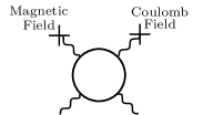
The advantage of this configuration is that it yields a large interaction volume, which goes along with a peak of the differential cross section for the vacuum birefringence signal in the forward direction.

2.2 Standard model

While in pure QED usually only the spinor-loop case is considered of direct phenomenological relevance, in QCD the scalar loop case can appear at low energies with a pion in the loop. In this connection, the scalar QED four-photon amplitude off-shell plays a central role in the dispersive approach to hadronic LBL scattering of [109]. When applied to the hadronic LBL contribution to the muon anomalous magnetic moment, this leads to the left-hand diagram of Fig. 3 with a pion loop (the same diagram appears with a quark loop in the OPE-based approach to the hadronic LBL contribution to $g-2$ of [110, 111, 112]).

The box diagram(s) with two photons and two gluons figure prominently in the recent study of the role of the chiral anomaly in polarized deeply inelastic scattering by A. Tarasov and R. Venugopalan [113] (also using the worldline formalism). This calculation is still not essentially different from the purely photonic one because with only two gluons the presence of the color factors does not yet make it necessary to fix an ordering of the four legs.

Similarly, the computation of the box diagram with three photons and one $Z$ can still be reduced to the one of the four-photon box since the axial part of the coupling of the $Z$ to the fermion line drops out in the sum of diagrams [114, 115]. With the three photons on-shell and the $Z$ off-shell it gives an important contribution to the process $\gamma\nu\rightarrow\gamma\gamma\nu$ and its crossed processes, see Fig. 10.

2.3 Beyond the standard model

The diagram of Fig. 10 has also been studied for the left-right symmetric extension of the SM with the $Z$ replaced by a $Z^{\prime}$ [116].

Another type of exotic particles suggested by BSM models are millicharged fermions. Those would contribute to the four-photon amplitude as loop particles in the same way as the standard model fermions. In particular, in a magnetic field they would lead to vacuum birefringence and dichroism, which has been used in [117] to obtain strong constraints on millicharged fermions from existing data on laser experiments.

Another recent application of light-by-light scattering is to the production of dark photons, a new candidate for dark matter [118].

3 Worldline representation of the $N$ -photon amplitudes

In the worldline approach to scalar QED, the $N$ -photon amplitude possesses the following path-integral representation:

	$\displaystyle\Gamma_{\rm scal}(k_{1},\varepsilon_{1};\ldots;k_{N},\varepsilon_{N})$	$\displaystyle=$	$\displaystyle(-ie)^{N}\int_{0}^{\infty}\frac{dT}{T}\,\,{\rm e}^{-m^{2}T}\int_{x(0)=x(T)}Dx\,\,{\rm e}^{-\int_{0}^{T}d\tau{1\over 4}\dot{x}^{2}}$
			$\displaystyle\times V_{\rm scal}^{\gamma}[k_{1},\varepsilon_{1}]\cdots V_{\rm scal}^{\gamma}[k_{N},\varepsilon_{N}]\,.$

Here $T$ is the proper-time of the scalar particle in the loop, and the path integral is performed over the space of all closed loops in (Euclidean) spacetime with periodicity $T$ . Each photon is represented by the following photon vertex operator, integrated along the trajectory:

\displaystyle V_{\rm scal}^{\gamma}[k,\varepsilon]

\displaystyle\equiv

\displaystyle\int_{0}^{T}d\tau\,\varepsilon\cdot\dot{x}(\tau)\,{\,{\rm e}}^{ik\cdot x(\tau)}\,.

(3.2)

The path integral is of gaussian form, and thus can be performed by Wick contractions in the one-dimensional worldline field theory. Using a formal exponentiation of the factor $\varepsilon\cdot\dot{x}=\,{\rm e}^{\varepsilon\cdot\dot{x}}|_{\varepsilon}$ , one straightforwardly arrives at the following “Bern-Kosower master formula”:

	$\displaystyle\Gamma_{\rm scal}(k_{1},\varepsilon_{1};\ldots;k_{N},\varepsilon_{N})$	$\displaystyle=$	$\displaystyle{(-ie)}^{N}{\int_{0}^{\infty}}\frac{dT}{T}{(4\pi T)}^{-\frac{D}{2}}\,{\rm e}^{-m^{2}T}\prod_{i=1}^{N}\int_{0}^{T}d\tau_{i}$
			$\displaystyle\hskip-42.67912pt\times\exp\biggl{\{}\sum_{i,j=1}^{N}\Bigl{[}{1\over 2}G_{ij}k_{i}\cdot k_{j}-i\dot{G}_{ij}\varepsilon_{i}\cdot k_{j}+{1\over 2}\ddot{G}_{ij}\varepsilon_{i}\cdot\varepsilon_{j}\Bigr{]}\biggr{\}}\Bigl{\|}_{\varepsilon_{1}\varepsilon_{2}\ldots\varepsilon_{N}}\,.$

Here the dependence on the proper-time parameters $T,\tau_{1},\ldots,\tau_{N}$ is encoded in the “worldline Green’s function”

\displaystyle G(\tau_{1},\tau_{2})=\mid\tau_{1}-\tau_{2}\mid-\frac{(\tau_{1}-\tau_{2})^{2}}{T}\,,

(3.4)

together with its first and second derivatives:

	$\displaystyle\dot{G}(\tau_{1},\tau_{2})$	$\displaystyle=$	$\displaystyle{\rm sgn}(\tau_{1}-\tau_{2})-2\frac{(\tau_{1}-\tau_{2})}{T}\,,$
	$\displaystyle\ddot{G}(\tau_{1},\tau_{2})$	$\displaystyle=$	$\displaystyle 2{\delta}(\tau_{1}-\tau_{2})-\frac{2}{T}\,.\quad$

Dots here denote a derivative acting on the first variable, $\dot{G}(\tau_{1},\tau_{2})\equiv\frac{\partial}{\partial\tau_{1}}G(\tau_{1},\tau_{2})$ , and we abbreviate $G_{ij}\equiv G(\tau_{i},\tau_{j})$ etc. The notation $\bigl{|}_{\varepsilon_{1}\varepsilon_{2}\ldots\varepsilon_{N}}$ means that, after the expansion of the exponential, only those terms should be kept that involve each polarization vector $\varepsilon_{1},\ldots,\varepsilon_{N}$ linearly. The fact that we are introducing these polarization vectors does not mean that we are imposing on-shell conditions; throughout this series of papers we will work fully off-shell, so that all polarization vectors will be arbitrary four-vectors used for notational convenience only.

Let us also emphasize already here that (LABEL:Nphotonvertop) and (LABEL:scalarqedmaster) represent the full $N$ -photon amplitude without the need of summing over permutations of the photon legs. What is more, the permutation (= Bose) symmetry is already manifest at the integrand level.

Proceeding to the spinor QED case, differently from the standard Dirac formalism in the worldline formalism the $N$ -photon amplitudes display a manifest break-up into contributions from the orbital and spin degrees of freedom of the loop fermion. The former are given by the same path integral as in the scalar QED case above, while for the latter there are various equivalent representations [34, 119, 120, 121]. In the present series of papers, we will follow the approach going back to Fradkin [119] where (LABEL:Nphotonvertop) gets generalized to

	$\displaystyle\Gamma_{\rm spin}(k_{1},\varepsilon_{1};\ldots;k_{N},\varepsilon_{N})$	$\displaystyle=$	$\displaystyle-{1\over 2}(-ie)^{N}\int_{0}^{\infty}\frac{dT}{T}\,\,{\rm e}^{-m^{2}T}\int_{P}Dx\,\,{\rm e}^{-\int_{0}^{T}d\tau{1\over 4}\dot{x}^{2}}$
			$\displaystyle\times\int_{A}D\psi(\tau)\,\,{\rm e}^{-\int_{0}^{T}d\tau{1\over 2}\psi\cdot\dot{\psi}}V^{\gamma}_{\rm spin}[k_{1},\varepsilon_{1}]\cdots V^{\gamma}_{\rm spin}[k_{N},\varepsilon_{N}]\,,\,$

where $P$ stands for “periodic boundary conditions” and $A$ for “anti-periodic boundary conditions”. Now $V^{\gamma}_{\rm spin}$ is the vertex operator for the emission or absorption of a photon by a spin-half particle (called “electron” for definiteness in the following)

\displaystyle V^{\gamma}_{\rm spin}[k,\varepsilon]

\displaystyle\equiv

\displaystyle\int_{0}^{T}d\tau\,\Bigl{[}\varepsilon\cdot\dot{x}(\tau)+2i\varepsilon\cdot\psi(\tau)k\cdot\psi(\tau)\Bigr{]}\,\,{\rm e}^{ik\cdot x(\tau)}\,.

(3.7)

The additional term, representing the interaction of the electron spin with the photon, is written in terms of a Grassmann-valued Lorentz vector $\psi^{\mu}(\tau)$ obeying anti-periodic boundary conditions, $\psi^{\mu}(T)=-\psi^{\mu}(0)$ . The Grassmann path integral can be evaluated by Wick contractions using the basic two-point correlator

\displaystyle\langle\psi^{\mu}(\tau)\psi^{\nu}(\tau^{\prime})\rangle

\displaystyle=

\displaystyle{1\over 2}G_{F}(\tau,\tau^{\prime})\delta^{\mu\nu}\,,

(3.8)

where

\displaystyle G_{F}(\tau,\tau^{\prime})\equiv{\rm sgn}(\tau-\tau^{\prime})\,.

(3.9)

The free Grassmann path integral is normalized to $4$ , the number of real degrees of freedom of the electron/positron in four-dimensions.

The worldline representation of the $N$ -photon amplitudes has been generalized to include a constant external field in [122, 123]. The generalization to the open-line case in scalar QED, i.e. the scalar propagator dressed with $N$ photons, was given in [124, 125], and extended to the constant-field case in [126]. Very recently, a computationally efficient worldline representation has also been constructed for the dressed electron propagator [127]. The formalism has also been applied to multiloop QED amplitudes [128, 123, 129, 130, 131, 132, 133, 125, 134].

Although in the present series of papers we focus on the QED photon amplitudes, it should be mentioned that Bern-Kosower type formulas have been derived also for many other cases. See [30, 135, 136] for the $N$ -gluon amplitudes in QCD, and [137, 138, 139] for amplitudes involving gravitons.

To start exploiting the master formula, we introduce polynomials $P_{N}$ capturing the result of the expansion of the exponential in (LABEL:scalarqedmaster) for fixed $N$ :

\displaystyle\exp\biggl{\{}\cdot\biggr{\}}\Bigl{|}_{\varepsilon_{1}\varepsilon_{2}\ldots\varepsilon_{N}}\quad\equiv{(-i)}^{N}P_{N}(\dot{G}_{ij},\ddot{G}_{ij})\exp\biggl{[}{1\over 2}\sum_{i,j=1}^{N}G_{ij}k_{i}\cdot k_{j}\biggr{]}\,.

(3.10)

However, in the worldline formalism one does not usually use this form of the integrand. Rather, one applies IBP to remove all second derivatives $\ddot{G}_{ij}$ of the worldline Green’s function from the integrand. This is always possible, and since $G(\tau,\tau^{\prime})$ is adapted to the periodic boundary conditions does not generate boundary terms. Thus the whole effect of the IBP is the replacement of $P_{N}(\dot{G}_{ij},\ddot{G}_{ij})$ by a new polynomial $Q_{N}(\dot{G}_{ij})$ . This polynomial is unique for $N=2$ and $N=3$ , while beginning with the four-point case different IBP procedures exist that lead to different equivalent results [35]. This ambiguity was discussed in [36] and a definite algorithm, called “symmetric partial integration”, given that maintains the full permutation symmetry at each step, and leads to a unique polynomial $Q_{N}$ . The main advantage from this transition of the “P-representation” to the “Q-representation” is that the IBP homogenizes the integrand; every term in $Q_{N}$ has $N$ factors of $\dot{G}_{ij}$ and $N$ factors of external momentum. This makes it possible to combine terms in the integrand related by gauge invariance, and write it more compactly in terms of the photon field strength tensors (1.5). Namely, $Q_{N}$ turns out to contain all possible traces of products of field strength tensors, which motivates the definition of a “Lorentz-cycle” $Z_{n}(i_{1}i_{2}\ldots i_{n})$ as

	$\displaystyle Z_{2}(ij)$	$\displaystyle\equiv$	$\displaystyle{1\over 2}{\rm tr}\bigl{(}f_{i}f_{j}\bigr{)}=\varepsilon_{i}\cdot k_{j}\varepsilon_{j}\cdot k_{i}-\varepsilon_{i}\cdot\varepsilon_{j}k_{i}\cdot k_{j}\,,$
	$\displaystyle Z_{n}(i_{1}i_{2}\ldots i_{n})$	$\displaystyle\equiv$	$\displaystyle{\rm tr}\Bigl{(}\prod_{j=1}^{n}f_{i_{j}}\Bigr{)}\,,\quad(n\geq 3)\,.$

Moreover, it turns out [35, 36] that in $Q_{N}$ each Lorentz-cycle $Z_{n}(i_{1}i_{2}\ldots i_{n})$ appears multiplied by a corresponding “ $\tau$ -cycle”

\displaystyle\dot{G}_{i_{1}i_{2}}\dot{G}_{i_{2}i_{3}}\cdots\dot{G}_{i_{n}i_{1}}\,.

(3.12)

This motivates the further definition of a “bicycle” as the product of the two:

\displaystyle\dot{G}(i_{1}i_{2}\cdots i_{n})\equiv\dot{G}_{i_{1}i_{2}}\dot{G}_{i_{2}i_{3}}\cdots\dot{G}_{i_{n}i_{1}}Z_{n}(i_{1}i_{2}\cdots i_{n})\,.

(3.13)

Note that these bicycles are not all independent, since they are invariant under the operations of cyclic permutations and inversion. Thus the number of independent cycles of length $n$ is $\frac{n!}{2n}$ . For example, for $n=4$ there are only three really different cycles, which can be chosen as $\dot{G}(1234)$ , $\dot{G}(1243)$ , and $\dot{G}(1324)$ .

However, $Q_{N}$ can (except for $N=2$ and in the low-energy limit, see below Section 8) not be written entirely in terms of bicycles and their products. Starting from $N=3$ there will be leftovers, called “ $n$ -tails” in the notation of [35], where $n$ , the “length” of the tail, denotes the number of polarization vectors involved in the tail. In general $Q_{N}$ will involve tails with length $n=1,2,\ldots,N-2$ . Thus for our present purposes we will need to know only the one- and two-tails. Those are given by

	$\displaystyle T(i)$	$\displaystyle\equiv$	$\displaystyle\sum_{r\neq i}\dot{G}_{ir}\varepsilon_{i}\cdot k_{r}\,,$		(3.14)
	$\displaystyle T(ij)$	$\displaystyle\equiv$	$\displaystyle{\sum_{{{r\neq i,s\neq j}}\atop{(r,s)\neq(j,i)}}}\dot{G}_{ir}\varepsilon_{i}\cdot k_{r}\dot{G}_{js}\varepsilon_{j}\cdot k_{s}+{1\over 2}\dot{G}_{ij}\varepsilon_{i}\cdot\varepsilon_{j}\Big{[}\sum_{r\neq i,j}\dot{G}_{ir}k_{i}\cdot k_{r}-\sum_{s\neq j,i}\dot{G}_{js}k_{j}\cdot k_{s}\Big{]}\,.$

Here it should be noted that $\dot{G}(\tau,\tau)=0$ , so that, for example, the term with $r=i$ drops out in the sum defining the one-tail. In the following, we leave it understood that terms containing a $\dot{G}_{ii}$ are to be dropped. For the two-tail, also some terms must be discarded that are non-zero, but would lead to the appearance of a two-cycle in the tail, and thus to an overcounting. With increasing length of the tails one has to impose an increasing number of such restrictions to eliminate all the cycles that would otherwise still be present in the tails; see [140] for the details. There also the tails have been worked out explicitly up to length four, which is what is needed for the six-photon amplitudes ¹¹1Apart from providing compactness, the tails also possess remarkable algebraic properties that become relevant only in the non-abelian case, where they open up an easy route to the computation of Berends-Giele currents in BCJ gauge [141], objects that are central in color-kinematics duality [142]..

After this repackaging of the integrand into cycles and tails, $Q_{N}$ for sizeable $N$ (which includes already the case $N=4$ ) becomes vastly more compact than $P_{N}$ . Another great advantage of the “Q-representation” is that it allows one to make the transition from scalar to spinor QED by a simple pattern-matching procedure, the “Bern-Kosower replacement rule” [30, 135]: after the removal of all $\ddot{G}_{ij}$ , the integrand for the $N$ -photon amplitude in spinor QED can be obtained from the scalar QED one by multiplying the whole amplitude by a global factor of “-2” (for statistics and degrees of freedom), and applying the following “cycle replacement rule”,

\displaystyle\dot{G}_{i_{1}i_{2}}\dot{G}_{i_{2}i_{3}}\cdots\dot{G}_{i_{n}i_{1}}\rightarrow\dot{G}_{i_{1}i_{2}}\dot{G}_{i_{2}i_{3}}\cdots\dot{G}_{i_{n}i_{1}}-G_{Fi_{1}i_{2}}G_{Fi_{2}i_{3}}\cdots G_{Fi_{n}i_{1}}\,,

(3.16)

which transforms the bicycle $\dot{G}(i_{1}i_{2}\cdots i_{n})$ into the “super-bicycle”

\dot{G}_{\rm S}(i_{1}i_{2}\cdots i_{n})=\Big{(}\dot{G}_{i_{1}i_{2}}\dot{G}_{i_{2}i_{3}}\cdots\dot{G}_{i_{n}i_{1}}-G_{Fi_{1}i_{2}}G_{Fi_{2}i_{3}}\cdots G_{Fi_{n}i_{1}}\Big{)}Z_{n}(i_{1}\cdots i_{n})\,.

(3.17)

See [140] for a proof that this rule correctly generates all the terms that in a direct calculation of the double path integral (LABEL:DNpointspin) would come from Wick contractions using (3.8). The replacement rule has its origin in a supersymmetry between the orbital and spin degrees of freedom of the electron, called “worldline supersymmetry” [35, 140] which generalizes the well-known supersymmetry of the non-relativistic Pauli-equation (in the original string-based approach of Bern and Kosower the rule was derived from worldsheet supersymmetry [30, 135]).

Alternatively, the worldline supersymmetry can also be used in a more direct way by the introduction of a worldline super formalism [32, 140, 143]. This allows one to write down the following spinor-QED analogue of the master formula (LABEL:scalarqedmaster),

	$\displaystyle\Gamma_{\rm spin}(k_{1},\varepsilon_{1};\ldots;k_{N},\varepsilon_{N})$	$\displaystyle=$	$\displaystyle-2{(-ie)}^{N}\int_{0}^{\infty}{dT\over T}{(4\pi T)}^{-{D\over 2}}\,{\rm e}^{-m^{2}T}$
			$\displaystyle\!\!\!\!\!\!\!\!\!\!\!\!\!\!\!\!\!\!\!\!\!\!\!\!\!\!\!\!\!\!\!\!\!\!\!\!\!\!\!\!\!\!\!\!\!\!\!\!\!\!\!\!\!\!\!\!\!\!\!\!\!\!\!\!\!\!\!\!\!\!\!\times\prod_{i=1}^{N}\int_{0}^{T}d\tau_{i}\int d\theta_{i}\exp\biggl{\{}\sum_{i,j=1}^{N}\Biggl{[}{1\over 2}\hat{G}_{ij}k_{i}\cdot k_{j}+iD_{i}\hat{G}_{ij}\varepsilon_{i}\cdot k_{j}+{1\over 2}D_{i}D_{j}\hat{G}_{ij}\varepsilon_{i}\cdot\varepsilon_{j}\Biggr{]}\biggr{\}}\mid_{\varepsilon_{1}\ldots\varepsilon_{N}}\,.$

Here the $\theta_{i}$ are Grassmann variables,

\displaystyle\hat{G}(\tau,\theta;\tau^{\prime},\theta^{\prime})\equiv G_{B}(\tau,\tau^{\prime})+\theta\theta^{\prime}G_{F}(\tau,\tau^{\prime})\,,

(3.19)

is the “worldline superpropagator”, and $D\equiv{\partial\over{\partial\theta}}-\theta{\partial\over{\partial\tau}}$ the super derivative.

4 The four-photon case

In the $N=4$ case, a direct expansion of the master formula (LABEL:scalarqedmaster) yields the “P-representation” of the scalar QED four-photon amplitude in $D$ dimensions:

	$\displaystyle\Gamma_{\rm scal}(k_{1},\varepsilon_{1};\ldots;k_{4},\varepsilon_{4})$	$\displaystyle=$	$\displaystyle e^{4}\int_{0}^{\infty}\frac{dT}{T}(4\pi T)^{-\frac{D}{2}}\,{\rm e}^{-m^{2}T}$
			$\displaystyle\times\int_{0}^{T}\prod_{i=1}^{4}d\tau_{i}\,P_{4}(\dot{G}_{ij},\ddot{G}_{ij})\,\exp\left[\sum_{i,j=1}^{4}{1\over 2}G_{ij}k_{i}\cdot k_{j}\right]\,,$

where

$\displaystyle P_{4}(\dot{G}_{ij},\ddot{G}_{ij})=$		$\displaystyle\ddot{G}_{12}\varepsilon_{1}\cdot\varepsilon_{2}\,\ddot{G}_{34}\varepsilon_{3}\cdot\varepsilon_{4}+\ddot{G}_{13}\varepsilon_{1}\cdot\varepsilon_{3}\,\ddot{G}_{24}\varepsilon_{2}\cdot\varepsilon_{4}+\ddot{G}_{14}\varepsilon_{1}\cdot\varepsilon_{4}\,\ddot{G}_{23}\varepsilon_{2}\cdot\varepsilon_{3}$
	$\displaystyle-$	$\displaystyle\dot{G}_{1i}\varepsilon_{1}\cdot k_{i}\,\dot{G}_{2j}\varepsilon_{2}\cdot k_{j}\,\ddot{G}_{34}\varepsilon_{3}\cdot\varepsilon_{4}-\dot{G}_{1i}\varepsilon_{1}\cdot k_{i}\,\dot{G}_{3j}\varepsilon_{3}\cdot k_{j}\,\ddot{G}_{24}\varepsilon_{2}\cdot\varepsilon_{4}$
	$\displaystyle-$	$\displaystyle\dot{G}_{1i}\varepsilon_{1}\cdot k_{i}\,\dot{G}_{4j}\varepsilon_{4}\cdot k_{j}\,\ddot{G}_{23}\varepsilon_{2}\cdot\varepsilon_{3}-\dot{G}_{2i}\varepsilon_{2}\cdot k_{i}\,\dot{G}_{3j}\varepsilon_{3}\cdot k_{j}\,\ddot{G}_{14}\varepsilon_{1}\cdot\varepsilon_{4}$
	$\displaystyle-$	$\displaystyle\dot{G}_{2i}\varepsilon_{2}\cdot k_{i}\,\dot{G}_{4j}\varepsilon_{4}\cdot k_{j}\,\ddot{G}_{13}\varepsilon_{1}\cdot\varepsilon_{3}-\dot{G}_{3i}\varepsilon_{3}\cdot k_{i}\,\dot{G}_{4j}\varepsilon_{4}\cdot k_{j}\,\ddot{G}_{12}\varepsilon_{1}\cdot\varepsilon_{2}$
	$\displaystyle+$	$\displaystyle\dot{G}_{1i}\varepsilon_{1}\cdot k_{i}\,\dot{G}_{2j}\varepsilon_{2}\cdot k_{j}\,\dot{G}_{3k}\varepsilon_{3}\cdot k_{k}\,\dot{G}_{4l}\varepsilon_{4}\cdot k_{l}\,.$

and the indices $i,j,k,l$ are to be summed from $1$ to $4$ . As described above, by IBP this can be transformed into the corresponding “Q-representation”,

\displaystyle\Gamma_{\rm scal}(k_{1},\varepsilon_{1};\ldots;k_{4},\varepsilon_{4})

\displaystyle=

\displaystyle e^{4}\int_{0}^{\infty}\frac{dT}{T}(4\pi T)^{-\frac{D}{2}}\,{\rm e}^{-m^{2}T}\int_{0}^{T}\prod_{i=1}^{4}d\tau_{i}\,Q_{4}(\dot{G}_{ij})\,\exp\left[\sum_{i,j=1}^{4}{1\over 2}G_{ij}k_{i}\cdot k_{j}\right]\,,

where now ²²2When comparing with [140] note that there a different basis was used for the four-cycle component $Q^{4}_{4}$ . The two bases are related by cyclicity and inversion.

$\displaystyle Q_{4}$	$\displaystyle=$	$\displaystyle Q^{4}_{4}+Q^{3}_{4}+Q^{2}_{4}+Q^{22}_{4}\,,$
$\displaystyle Q^{4}_{4}$	$\displaystyle=$	$\displaystyle\dot{G}(1234)+\dot{G}(2314)+\dot{G}(3124)\,,$
$\displaystyle Q^{3}_{4}$	$\displaystyle=$	$\displaystyle\dot{G}(123)T(4)+\dot{G}(234)T(1)+\dot{G}(341)T(2)+\dot{G}(412)T(3)\,,$
$\displaystyle Q^{2}_{4}$	$\displaystyle=$	$\displaystyle\dot{G}(12)T(34)+\dot{G}(13)T(24)+\dot{G}(14)T(23)+\dot{G}(23)T(14)+\dot{G}(24)T(13)+\dot{G}(34)T(12)\,,$
$\displaystyle Q^{22}_{4}$	$\displaystyle=$	$\displaystyle\dot{G}(12)\dot{G}(34)+\dot{G}(13)\dot{G}(24)+\dot{G}(14)\dot{G}(23)\,.$

Although this is already an extremely nice and compact representation of this amplitude, at this stage it is natural to ask whether further IBP might exist that would allow one to absorb into field-strength tensors not only the polarization vectors contained in the cycles, but also those in the tails. It turns out that this is indeed possible, at the cost of introducing inverse factors of momenta in the IBP, and a set of (almost) arbitrary auxiliary vectors $r_{i}^{\mu}$ . In [37] it was shown how to rewrite, by suitable such IBPs involving only the tail variables, a tail of arbitrary length completely in terms of field strength tensors. The resulting representation of the scalar and spinor QED photon amplitudes, which has the remarkable property of being manifestly transversal already at the integrand level, was called “QR-representation”. For our purposes, we will need only the corresponding form of the one-tail:

\displaystyle T_{R}(i)

\displaystyle\equiv

\displaystyle\sum_{j\neq i}\dot{G}_{ij}~{}\frac{r_{i}\cdot f_{i}\cdot k_{j}}{r_{i}\cdot k_{i}}\,.

(4.5)

The vector $r_{i}$ , called “reference vector”, is arbitrary except that it has to obey $r_{i}\cdot k_{i}\neq 0$ . To obtain (4.5) from (3.14), one needs a single total derivative term:

\displaystyle T_{R}(i)\,\,{\rm e}^{(\cdot)}=T(i)\,\,{\rm e}^{(\cdot)}-\partial_{i}\Bigl{(}\frac{r_{i}\cdot\varepsilon_{i}}{r_{i}\cdot k_{i}}\,\,{\rm e}^{(\cdot)}\Bigr{)}\,.

(4.6)

Here we have introduced the abbreviations $\partial_{i}\equiv\frac{d}{d\tau_{i}}$ and

\displaystyle\,{\rm e}^{(\cdot)}\equiv\exp\left[\sum_{i,j=1}^{4}{1\over 2}G_{ij}k_{i}\cdot k_{j}\right]\,.

(4.7)

The choice of the reference vector for most purposes should be done in such a way that the permutation symmetry between the photons with index other than $i$ remains unbroken. Since one usually would like to avoid introducing new vectors, a natural choice is $r_{i}=k_{i}$ , however this creates a $k_{i}^{2}$ in the denominator, and thus a spurious singularity in the on-shell limit. Alternatively, one could use each of the remaining photon momenta and take the average of the resulting integrals.

For the two-tail, various versions were obtained in [37], but here we will rather introduce a new one, the “short two-tail” $T_{sh}(ij)$ , that we have found much superior to those. It is defined by

\displaystyle T_{sh}(ij)\equiv\sum_{r,s\neq i,j}\dot{G}_{ri}\dot{G}_{js}~{}\frac{k_{r}\cdot f_{i}\cdot f_{j}\cdot k_{s}}{k_{i}\cdot k_{j}}\,,

(4.8)

and obtained from the Q-version of the two-tail (3) by adding the following set of total derivative terms,

	$\displaystyle T_{sh}(ij)\,\,{\rm e}^{(\cdot)}$	$\displaystyle=$	$\displaystyle T(ij)\,\,{\rm e}^{(\cdot)}+\frac{1}{k_{i}\cdot k_{j}}\biggl{[}\varepsilon_{i}\cdot\varepsilon_{j}\,\partial_{i}\partial_{j}\,\,{\rm e}^{(\cdot)}-\varepsilon_{i}\cdot k_{j}\varepsilon_{j}\cdot k_{s}\partial_{i}\Bigl{(}\dot{G}_{js}\,\,{\rm e}^{(\cdot)}\Bigr{)}$
			$\displaystyle-\varepsilon_{j}\cdot k_{i}\varepsilon_{i}\cdot k_{r}\partial_{j}\Bigl{(}\dot{G}_{ir}\,\,{\rm e}^{(\cdot)}\Bigr{)}+\Bigl{(}{1\over 2}\varepsilon_{i}\cdot\varepsilon_{j}k_{i}\cdot k_{j}-\varepsilon_{i}\cdot k_{j}\varepsilon_{j}\cdot k_{i}\Bigr{)}(\partial_{i}-\partial_{j})\Bigl{(}\dot{G}_{ij}\,\,{\rm e}^{(\cdot)}\Bigr{)}\biggr{]}\,,$

( $i,j$ fixed, $r,s$ summed over). Note that the indices $r,s$ in (4.8) now take only values in the cycle variables, thus there are only four terms instead of twelve as compared to the Q-tail (3). This explains the name “short tail”. Thus when we have the short two-tail and the Q one-tail the representation will be called “STQ-representation”. The manifestly transversal representation comes with the short two-tail and the R one-tail, being then the “STR-representation”. Let us process the integrand a bit further by the standard rescaling

\displaystyle\tau_{i}=Tu_{i},\quad i=1,\ldots,4\,.

(4.10)

We can then write the four-photon amplitudes, combined for scalar and spinor QED, in the following way:

\displaystyle\Gamma_{\{{{\rm scal}\atop{\rm spin}}\}}(k_{1},\varepsilon_{1};\ldots;k_{4},\varepsilon_{4})

\displaystyle=

\displaystyle\Big{\{}{{1}\atop{-2}}\Big{\}}\frac{e^{4}}{(4\pi)^{\frac{D}{2}}}\int_{0}^{\infty}\frac{dT}{T}T^{4-\frac{D}{2}}\,{\rm e}^{-m^{2}T}\int_{0}^{1}\prod_{i=1}^{4}du_{i}\,Q_{\{{{\rm scal}\atop{\rm spin}}\}}(\dot{G}_{ij})\,\,{\rm e}^{(\cdot)}\,.

The prefactor polynomial for scalar QED, $Q_{\rm scal}(\dot{G}_{ij})$ , is given by (LABEL:q4) with the cycles defined in (3.13) and the tails defined in (4.5) and (4.8) (here and in the following we will often drop the subscript ‘4’ on $Q$ ). The one for spinor QED, $Q_{\rm spin}(\dot{G}_{ij})$ , has all bicycle factors replaced by the super-bicycle factors (3.17). Note that we do not introduce a new symbol for the worldline Green’s function after the rescaling, which is now given by

\displaystyle G_{ij}=|u_{i}-u_{j}|-(u_{i}-u_{j})^{2}\,.

(4.12)

Note further that $T$ appears linearly in the rescaled exponent,

\displaystyle\,{\rm e}^{(\cdot)}\equiv\exp\left[\sum_{i,j=1}^{4}\frac{T}{2}G_{ij}k_{i}\cdot k_{j}\right]\,.

(4.13)

It should be clear from the context whether the original or the rescaled Green’s function is to be used. We will also often strip off the global prefactors of the amplitude, defining

\displaystyle\Gamma_{\{{{\rm scal}\atop{\rm spin}}\}}

\displaystyle\equiv

\displaystyle\Big{\{}{{1}\atop{-2}}\Big{\}}\frac{e^{4}}{(4\pi)^{\frac{D}{2}}}\hat{\Gamma}_{\{{{\rm scal}\atop{\rm spin}}\}}\,.

(4.14)

5 Worldline vs. Feynman diagram representations

Next, let us discuss the relation between the parameter integrals appearing in the worldline representation of the $N$ -photon amplitudes and the parameter integrals arising in the calculation of the corresponding Feynman diagrams using Feynman-Schwinger parameters.

In scalar QED, the parameter integrals of the P-representation, obtained directly from the expansion of the master formula (LABEL:scalarqedmaster), can, for a fixed ordering of the legs, straightforwardly be identified with the ones of the Feynman-Schwinger parameter integral representation of the corresponding Feynman diagrams.

E.g. for the “standard” ordering of the legs the transformation can be read off from Fig. 11. Using the translation invariance in the proper-time to set $\tau_{N}=0$ , and choosing the parametrization of the loop such that $T\geq\tau_{1}\geq\tau_{2}\geq\ldots\tau_{N}=0$ , one gets

$\displaystyle\tau_{1}$	$\displaystyle=$	$\displaystyle\alpha_{2}+\alpha_{3}+\ldots+\alpha_{N}\,,$
$\displaystyle\tau_{2}$	$\displaystyle=$	$\displaystyle\alpha_{3}+\alpha_{4}+\ldots+\alpha_{N}\,,$
$\displaystyle\vdots\,$		$\displaystyle\quad\vdots$
$\displaystyle\tau_{N-1}$	$\displaystyle=$	$\displaystyle\alpha_{N}\,.$

The $\delta(\tau_{i}-\tau_{j})$ in a $\ddot{G}_{ij}$ brings together photons $i$ and $j$ and thus creates a quartic vertex that corresponds to the seagull vertex in the standard formalism. It contributes only if legs $i$ and $j$ are adjacent for this ordering, and has to be split equally between the two sectors $\tau_{i}>\tau_{j}$ and $\tau_{i}<\tau_{j}$ .

In our $N=4$ case, the transformation (LABEL:tautoalpha) leads to the following formulas for the various worldline Green’s functions and their derivatives:

$\displaystyle G_{12}$	$\displaystyle=$	$\displaystyle\alpha_{2}(1-\alpha_{2})\hskip 62.59596pt,\hskip 14.22636pt\dot{G}_{12}=1-2\alpha_{2}\,,$
$\displaystyle G_{13}$	$\displaystyle=$	$\displaystyle(\alpha_{1}+\alpha_{4})(1-\alpha_{1}-\alpha_{4})~{}~{}~{},\hskip 8.5359pt\dot{G}_{31}=1-2(\alpha_{1}+\alpha_{4})\,,$
$\displaystyle G_{14}$	$\displaystyle=$	$\displaystyle\alpha_{1}(1-\alpha_{1})\hskip 62.59596pt,\hskip 14.22636pt\dot{G}_{41}=1-2\alpha_{1}\,,$
$\displaystyle G_{23}$	$\displaystyle=$	$\displaystyle\alpha_{3}(1-\alpha_{3})\hskip 62.59596pt,\hskip 14.22636pt\dot{G}_{23}=1-2\alpha_{3}\,,$
$\displaystyle G_{24}$	$\displaystyle=$	$\displaystyle(\alpha_{1}+\alpha_{2})(1-\alpha_{1}-\alpha_{2})\hskip 8.5359pt,\hskip 8.5359pt\dot{G}_{24}=1-2(\alpha_{3}+\alpha_{4})\,,$
$\displaystyle G_{34}$	$\displaystyle=$	$\displaystyle\alpha_{4}(1-\alpha_{4})\hskip 62.59596pt,\hskip 14.22636pt\dot{G}_{34}=1-2\alpha_{4}\,,$

and the exponential factor can, using momentum conservation, be identified with the standard four-point denominator of the Feynman-Schwinger representation,

\displaystyle\sum_{i<j=1}^{4}G_{ij}k_{i}\cdot k_{j}

\displaystyle=

\displaystyle-\alpha_{1}\alpha_{2}k_{1}^{2}-\alpha_{2}\alpha_{3}k_{2}^{2}-\alpha_{3}\alpha_{4}k_{3}^{2}-\alpha_{1}\alpha_{4}k_{4}^{2}-\alpha_{2}\alpha_{4}(k_{1}+k_{4})^{2}-\alpha_{1}\alpha_{3}(k_{1}+k_{2})^{2}\,.

Setting $\tau_{4}=0$ , splitting the remaining three $\tau$ -integrals into the six ordered sectors

$\displaystyle{\rm sector}\,1$	$\displaystyle:$	$\displaystyle\tau_{1}\geq\tau_{2}\geq\tau_{3}\geq\tau_{4}=0\,,$
$\displaystyle{\rm sector}\,2$	$\displaystyle:$	$\displaystyle\tau_{1}\geq\tau_{3}\geq\tau_{2}\geq\tau_{4}=0\,,$
$\displaystyle{\rm sector}\,3$	$\displaystyle:$	$\displaystyle\tau_{3}\geq\tau_{1}\geq\tau_{2}\geq\tau_{4}=0\,,$
$\displaystyle{\rm sector}\,4$	$\displaystyle:$	$\displaystyle\tau_{3}\geq\tau_{2}\geq\tau_{1}\geq\tau_{4}=0\,,$
$\displaystyle{\rm sector}\,5$	$\displaystyle:$	$\displaystyle\tau_{2}\geq\tau_{3}\geq\tau_{1}\geq\tau_{4}=0\,,$
$\displaystyle{\rm sector}\,6$	$\displaystyle:$	$\displaystyle\tau_{2}\geq\tau_{1}\geq\tau_{3}\geq\tau_{4}=0\,,$

and applying in each sector the appropriate transformation rule, one would arrive at the same collection of $\alpha$ - parameter integrals as in the calculation of the familiar sum of six diagrams shown in Fig. 12

and the terms involving $\delta$ functions would correspond precisely to the additional diagrams that one has in the scalar QED case involving one or two seagull vertices, see Fig. 13.

This makes it also clear that, in a straightforward use of the P-representation along these lines, we would not achieve much of an advantage over a standard Feynman-Schwinger parameter calculation. To improve on the standard method, it is essential to recognize, following [30, 135, 35], that the integrand of the P-representation is written in a form that suggests a removal of the $\ddot{G}_{ij}$ s by IBP. The resulting Q-representation (LABEL:4-photonQ) possesses already very substantive advantages over the standard one, which we can summarize as follows:

1.

It represent already the complete four-photon amplitude in scalar QED, corresponding to the sum of all the Feynman diagrams shown in Figs. 12 and 13.
2.

When rewritten in terms of Feynman-Schwinger parameters, the worldline integrals will still be of the same type that one would encounter in a Feynman diagram calculation. Nevertheless, due to the rearrangement into cycles and tails the worldline integrand will still be much more compact than what one would find in any straightforward diagrammatic calculation.
3.

As is well-known, the four-photon amplitudes in both scalar and spinor QED suffer from spurious UV divergences that cancel out in the sum of all Feynman diagrams by gauge invariance ³³3It is well-known that in QED gauge invariance can get lost if divergences are not handled with due care. See, e.g., [144].. In the P-representation, those divergences are still there and contained in the terms involving products of two $\ddot{G}_{ij}$ s, but they get removed by the IBP procedure; in the Q-representation all integrals are already finite term by term.
4.

The arrangement into cycles and tails allows one to obtain the corresponding spinor QED amplitude trivially by the application of the replacement rule (3.16). Thus effectively one bypasses all the Dirac-algebra manipulations of the standard approach.

After transforming to the improved tails (4.5) and (4.8), one gets the further advantage of manifest gauge invariance at the integrand level.

6 Minimal tensor bases for the four-photon amplitudes

For off-shell amplitudes, it is usually useful to have a tensor decomposition which is minimal (without redundancies) and compatible with all their symmetries. For our four-photon amplitude, the only symmetry around is the permutation (= Bose) symmetry between the photons. Thus we will now study how many independent tensor structures are contained in the worldline representation of the amplitude.

Clearly, in the decomposition (LABEL:q4) the terms $Q^{4}$ , $Q^{3}$ and $Q^{22}$ count only as one structure each, once permutations are taken into account. Thus only $Q^{2}$ needs to be analyzed, and here all six terms are related by permutations, so it is sufficient to analyze the first one, that is $\dot{G}(12)T_{sh}(34)$ in the scalar and $\dot{G}_{S}(12)T_{sh}(34)$ in the spinor QED case. Writing out $T_{sh}(34)$

\displaystyle T_{sh}(34)

\displaystyle=

\displaystyle\sum_{r,s=1,2}\dot{G}_{r3}\dot{G}_{4s}~{}\frac{k_{r}\cdot f_{3}\cdot f_{4}\cdot k_{s}}{k_{3}\cdot k_{4}}\,,

(6.1)

gives four terms, but they are not all independent, due to the symmetry $1\leftrightarrow 2$ of the cycle factor $\dot{G}_{(S)}(12)$ that leads to the equivalences

	$\displaystyle r=s=1$	$\displaystyle\sim$	$\displaystyle r=s=2\,,$
	$\displaystyle r=1,s=2$	$\displaystyle\sim$	$\displaystyle r=2,s=1\,.$

Thus the total number of independent tensor structures is five. We will label them in the following way:

$\displaystyle T^{(1)}_{(1234)}$	$\displaystyle\equiv$	$\displaystyle Z_{4}(1234)\,,$
$\displaystyle T^{(2)}_{(12)(34)}$	$\displaystyle\equiv$	$\displaystyle Z_{2}(12)Z_{2}(34)\,,$
$\displaystyle T^{(3)r_{4}}_{(123)i}$	$\displaystyle\equiv$	$\displaystyle Z_{3}(123)\frac{r_{4}\cdot f_{4}\cdot k_{i}}{r_{4}\cdot k_{4}}\,,\quad i=1,2,3\,,$
$\displaystyle T^{(4)}_{(12)ii}$	$\displaystyle\equiv$	$\displaystyle Z_{2}(12)\,\frac{k_{i}\cdot f_{3}\cdot f_{4}\cdot k_{i}}{k_{3}\cdot k_{4}}\,,\quad i=1,2,$
$\displaystyle T^{(5)}_{(12)ij}$	$\displaystyle\equiv$	$\displaystyle Z_{2}(12)\,\frac{k_{i}\cdot f_{3}\cdot f_{4}\cdot k_{j}}{k_{3}\cdot k_{4}}\,,\quad(i,j)=(1,2),(2,1).$

For completeness, let us also write down the full set of permutations of these tensors that will appear in the tensor decomposition:

	$\displaystyle T^{(1)}_{(1234)},T^{(1)}_{(1243)},T^{(1)}_{(1324)},T^{(2)}_{(12)(34)},T^{(2)}_{(13)(24)},T^{(2)}_{(14)(23)},$
	$\displaystyle T^{(3)r_{4}}_{(123)1},T^{(3)r_{4}}_{(123)2},T^{(3)r_{4}}_{(123)3},T^{(3)r_{1}}_{(234)2},T^{(3)r_{1}}_{(234)3},T^{(3)r_{1}}_{(234)4},T^{(3)r_{2}}_{(341)3},T^{(3)r_{2}}_{(341)4},T^{(3)r_{2}}_{(341)1},T^{(3)r_{3}}_{(4,1,2)4},T^{(3)r_{3}}_{(4,1,2)1},T^{(3)r_{3}}_{(4,1,2)2},$
	$\displaystyle T^{(4)}_{(12)11},T^{(4)}_{(12)22},T^{(4)}_{(13)11},T^{(4)}_{(13)33},T^{(4)}_{(14)11},T^{(4)}_{(14)44},T^{(4)}_{(23)22},T^{(4)}_{(23)33},T^{(4)}_{(24)22},T^{(4)}_{(24)44},T^{(4)}_{(34)33},T^{(4)}_{(34)44},$
	$\displaystyle T^{(5)}_{(12)12},T^{(5)}_{(12)21},T^{(5)}_{(13)13},T^{(5)}_{(13)31},T^{(5)}_{(14)14},T^{(5)}_{(14)41},T^{(5)}_{(23)23},T^{(5)}_{(23)32},T^{(5)}_{(24)24},T^{(5)}_{(24)42},T^{(5)}_{(34)34},T^{(5)}_{(34)43}\,.$

Note that these five tensors (we call them tensors since eventually the polarization vectors have to be stripped off) all have the same mass dimension, and that $T^{(3)r_{4}}_{(123)i}$ still depends on the choice of a reference momentum $r_{4}$ (which must not depend on $i$ ). $T^{(1)}$ and $T^{(2)}$ appear in three permutations, $T^{(3)}$ , $T^{(4)}$ and $T^{(5)}$ in twelve each. The complete four-photon amplitude can thus be decomposed as

\displaystyle\hat{\Gamma}

\displaystyle=

\displaystyle\hat{\Gamma}^{(1)}+\hat{\Gamma}^{(2)}+\hat{\Gamma}^{(3)}+\hat{\Gamma}^{(4)}+\hat{\Gamma}^{(5)}\,,

(6.5)

$\displaystyle\hat{\Gamma}^{(1)}$	$\displaystyle=$	$\displaystyle\hat{\Gamma}^{(1)}_{(1234)}T^{(1)}_{(1234)}+\hat{\Gamma}^{(1)}_{(1243)}T^{(1)}_{(1243)}+\hat{\Gamma}^{(1)}_{(1324)}T^{(1)}_{(1324)}\,,$
$\displaystyle\hat{\Gamma}^{(2)}$	$\displaystyle=$	$\displaystyle\hat{\Gamma}^{(2)}_{(12)(34)}T^{(2)}_{(12)(34)}+\hat{\Gamma}^{(2)}_{(13)(24)}T^{(2)}_{(13)(24)}+\hat{\Gamma}^{(2)}_{(14)(23)}T^{(2)}_{(14)(23)}\,,$
$\displaystyle\hat{\Gamma}^{(3)}$	$\displaystyle=$	$\displaystyle\sum_{i=1,2,3}\hat{\Gamma}^{(3)}_{(123)i}T^{(3)r_{4}}_{(123)i}+\sum_{i=2,3,4}\hat{\Gamma}^{(3)}_{(234)i}T^{(3)r_{1}}_{(234)i}+\sum_{i=3,4,1}\hat{\Gamma}^{(3)}_{(341)i}T^{(3)r_{2}}_{(341)i}+\sum_{i=4,1,2}\hat{\Gamma}^{(3)}_{(412)i}T^{(3)r_{3}}_{(412)i}\,,$
$\displaystyle\hat{\Gamma}^{(4)}$	$\displaystyle=$	$\displaystyle\sum_{i<j}\hat{\Gamma}^{(4)}_{(ij)ii}T^{(4)}_{(ij)ii}+\sum_{i<j}\hat{\Gamma}^{(4)}_{(ij)jj}T^{(4)}_{(ij)jj}\,,$
$\displaystyle\hat{\Gamma}^{(5)}$	$\displaystyle=$	$\displaystyle\sum_{i<j}\hat{\Gamma}^{(5)}_{(ij)ij}T^{(5)}_{(ij)ij}+\sum_{i<j}\hat{\Gamma}^{(5)}_{(ij)ji}T^{(5)}_{(ij)ji}\,.$

The coefficient functions are given, with the convention (4.14), by

\displaystyle\hat{\Gamma}^{(k)}_{\cdots}

\displaystyle=

\displaystyle\int_{0}^{\infty}\frac{dT}{T}T^{4-\frac{D}{2}}\,{\rm e}^{-m^{2}T}\int_{0}^{1}\prod_{i=1}^{4}du_{i}\,\hat{\gamma}^{(k)}_{\ldots}(\dot{G}_{ij})\,\,{\rm e}^{(\cdot)}\,,

where, for spinor QED,

$\displaystyle\hat{\gamma}^{(1)}_{(1234)}$	$\displaystyle=$	$\displaystyle\dot{G}_{12}\dot{G}_{23}\dot{G}_{34}\dot{G}_{41}-G_{F12}G_{F23}G_{F34}G_{F41}\,,$
$\displaystyle\hat{\gamma}^{(2)}_{(12)(34)}$	$\displaystyle=$	$\displaystyle\bigl{(}\dot{G}_{12}\dot{G}_{21}-G_{F12}G_{F21}\bigr{)}\bigl{(}\dot{G}_{34}\dot{G}_{43}-G_{F34}G_{F43}\bigr{)}\,,$
$\displaystyle\hat{\gamma}^{(3)}_{(123)1}$	$\displaystyle=$	$\displaystyle\bigl{(}\dot{G}_{12}\dot{G}_{23}\dot{G}_{31}-G_{F12}G_{F23}G_{F31}\bigr{)}\dot{G}_{41}\,,$
$\displaystyle\hat{\gamma}^{(4)}_{(12)11}$	$\displaystyle=$	$\displaystyle\bigl{(}\dot{G}_{12}\dot{G}_{21}-G_{F12}G_{F21}\bigr{)}\dot{G}_{13}\dot{G}_{41}\,,$
$\displaystyle\hat{\gamma}^{(5)}_{(12)12}$	$\displaystyle=$	$\displaystyle\bigl{(}\dot{G}_{12}\dot{G}_{21}-G_{F12}G_{F21}\bigr{)}\dot{G}_{13}\dot{G}_{42}$
			(6.8)

(plus permutations thereof), and the coefficient functions for scalar QED are obtained from these simply by deleting all the $G_{Fij}$ .

A further option is to use the trivial but highly useful identity

\displaystyle\dot{G}_{ij}^{2}=1-4G_{ij}\,,

(6.9)

to rewrite

\displaystyle\dot{G}_{ij}\dot{G}_{ji}-G_{Fij}G_{Fji}=4G_{ij}\,.

(6.10)

This will be useful not only for compactness, but also because factors of $G_{ij}$ can be generated by derivatives applied to the universal exponential factor. We can then replace (6.8) by the remarkably compact expressions

$\displaystyle\hat{\gamma}^{(1)}_{(1234)}$	$\displaystyle=$	$\displaystyle\dot{G}_{12}\dot{G}_{23}\dot{G}_{34}\dot{G}_{41}-G_{F12}G_{F23}G_{F34}G_{F41}\,,$
$\displaystyle\hat{\gamma}^{(2)}_{(12)(34)}$	$\displaystyle=$	$\displaystyle 16G_{12}G_{34}\,,$
$\displaystyle\hat{\gamma}^{(3)}_{(123)1}$	$\displaystyle=$	$\displaystyle\bigl{(}\dot{G}_{12}\dot{G}_{23}\dot{G}_{31}-G_{F12}G_{F23}G_{F31}\bigr{)}\dot{G}_{41}\,,$
$\displaystyle\hat{\gamma}^{(4)}_{(12)11}$	$\displaystyle=$	$\displaystyle 4G_{12}\dot{G}_{13}\dot{G}_{41}\,,$
$\displaystyle\hat{\gamma}^{(5)}_{(12)12}$	$\displaystyle=$	$\displaystyle 4G_{12}\dot{G}_{13}\dot{G}_{42}\,.$

Finally, let us compare our basis of invariants with the one obtained in [27] in a very different way, namely by writing down all possible tensor structures and systematically reducing them by the application of the Ward identity and the permutation group. This also led them to a basis composed of five gauge-invariant tensors $I_{\mu\nu\rho\sigma}^{(i)}$ , chosen as

I_{\mu\nu\rho\sigma}^{(1)}(1234)=\frac{1}{32}F_{\mu\alpha\beta}(1)F_{\nu\beta\alpha}(2)F_{\rho\gamma\delta}(3)F_{\sigma\delta\gamma}(4)\,,

(6.12)

I_{\mu\nu\rho\sigma}^{(2)}(1234)=\frac{1}{8}F_{\mu\alpha\beta}(1)F_{\nu\beta\gamma}(2)F_{\rho\gamma\delta}(3)F_{\sigma\delta\alpha}(4)\,,

(6.13)

I_{\mu\nu\rho\sigma}^{(3)}(1234)=-\frac{1}{4(k^{(3)}k^{(4)})}F_{\mu\alpha\beta}(1)F_{\nu\beta\alpha}(2)k_{\gamma}F_{\rho\gamma\delta}(3)F_{\sigma\delta\xi}(4)k_{\xi}^{(1)}\,,

(6.14)

I_{\mu\nu\rho\sigma}^{(4)}(1234)=-\frac{1}{4(k^{(3)}k^{(4)})}F_{\mu\alpha\beta}(1)F_{\nu\beta\alpha}(2)k_{\gamma}^{(2)}F_{\rho\gamma\delta}(3)F_{\sigma\delta\xi}(4)k_{\xi}^{(1)}\,,

(6.15)

I_{\mu\nu\rho\sigma}^{(5)}(1234)=\frac{1}{3(k^{(2)}k^{(4)})}k_{\alpha}^{(2)}F_{\sigma\alpha\beta}(4)F_{\mu\beta\gamma}(1)\Big{[}F_{\nu\gamma\delta}(2)F_{\rho\delta\xi}(3)-F_{\rho\gamma\delta}(3)F_{\nu\delta\xi}(2)\Big{]}k_{\xi}^{(1)}\,.

(6.16)

Here the third-rank tensor $F_{\eta\mu\nu}(i)$ is defined by

F_{\eta\mu\nu}(i)=-F_{\eta\nu\mu}(i)=\delta_{\eta\mu}k_{\nu}^{(i)}-\delta_{\eta\nu}k_{\mu}^{(i)}\,,

(6.17)

which is related to (1.5) by

\varepsilon_{\eta}^{(i)}F_{\eta\mu\nu}(i)=f_{i}^{\nu\mu}\,.

(6.18)

Let us define

I^{(i)}\equiv\varepsilon_{\mu}^{(1)}\varepsilon_{\nu}^{(2)}\varepsilon_{\rho}^{(3)}\varepsilon_{\sigma}^{(4)}I_{\mu\nu\rho\sigma}^{(i)}\,.

(6.19)

We can then write the five gauge-invariant tensors $I^{(i)}$ in terms of the field strength tensors $f_{i}$ as follows:

I^{(1)}(1234)=\frac{1}{32}{\rm tr}(f_{1}f_{2}){\rm tr}(f_{3}f_{4})\,,

(6.20)

I^{(2)}(1234)=\frac{1}{8}{\rm tr}(f_{1}f_{2}f_{3}f_{4})\,,

(6.21)

I^{(3)}(1234)=-\frac{1}{4k_{3}\cdot k_{4}}{\rm tr}(f_{1}f_{2})k_{1}\cdot f_{3}\cdot f_{4}\cdot k_{1}\,,

(6.22)

I^{(4)}(1234)=-\frac{1}{4k_{3}\cdot k_{4}}{\rm tr}(f_{1}f_{2})k_{2}\cdot f_{3}\cdot f_{4}\cdot k_{1}\,,

(6.23)

I^{(5)}(1234)=\frac{1}{3k_{2}\cdot k_{4}}k_{2}\cdot f_{4}\cdot k_{1}~{}{\rm tr}(f_{1}f_{2}f_{3})\,.

(6.24)

It thus becomes apparent that this basis $\{I^{(i)}\}$ differs from our basis $\{T^{(i)}\}$ only by some rescaling:

$\displaystyle T^{(1)}_{(1234)}$	$\displaystyle=$	$\displaystyle 8I^{(2)}(1234)\,,$
$\displaystyle T^{(2)}_{(12)(34)}$	$\displaystyle=$	$\displaystyle 8I^{(1)}(1234)\,,$
$\displaystyle T^{(3)k_{2}}_{(123)1}$	$\displaystyle=$	$\displaystyle 3I^{(5)}(1234)\,,$
$\displaystyle T^{(4)}_{(12)11}$	$\displaystyle=$	$\displaystyle-2I^{(3)}(1234)\,,$
$\displaystyle T^{(5)}_{(12)12}$	$\displaystyle=$	$\displaystyle-2I^{(4)}(2134)\,.$

Note, however, that for $T^{(3)}$ to match with $I^{(5)}$ we had to choose the reference momentum of the one-tail as one of the momenta of the other photons, which is, of course, not obligatory. In this sense our basis is slightly more general than the one of [27].

We find it remarkable that our IBP procedure, whose main purpose was to write the integrand of the four-photon amplitudes in the most compact possible way, has led to the emergence of the same tensor basis that was found by [27] using the Ward identity.

It must be noted, though, that the price to pay for this optimization is the introduction of the tensors $T^{(4)}$ and $T^{(5)}$ that carry denominators, and thus introduce spurious kinematic singularities. It is easy to see that this cannot be avoided if one wishes the basis to be minimal as well as manifestly transversal. For some purposes it may be preferable to use a tensor basis that is less optimized but free of kinematic singularities [109].

7 Matching identities

Useful identities can be derived by comparing the worldline integrands before and after the IBP procedure. The key observation is that the terms involving purely products of $\ddot{G}_{ij}$ resp. $D_{i}D_{j}\hat{G}_{ij}$ in the master formulas (LABEL:scalarqedmaster) and (LABEL:supermaster) involve only scalar integrals, and are thus trivial from the point of view of tensor reduction. We will now work this out for the four-photon case, using the notation

	$\displaystyle\hat{I}_{n}^{D}(k_{1},\ldots,k_{n})$	$\displaystyle\equiv$	$\displaystyle\int_{0}^{\infty}\frac{dT}{T}T^{n-\frac{D}{2}}\,{\rm e}^{-m^{2}T}\prod_{i=1}^{n}\int_{0}^{1}du_{i}\,{\rm e}^{T\sum_{i<j=1}^{n}G_{ij}k_{ij}}\,,$
	$\displaystyle\hat{I}_{n}^{D}(k_{1},\ldots,k_{n})[X]$	$\displaystyle\equiv$	$\displaystyle\int_{0}^{\infty}\frac{dT}{T}T^{n-\frac{D}{2}}\,{\rm e}^{-m^{2}T}\prod_{i=1}^{n}\int_{0}^{1}du_{i}\,X\,{\rm e}^{T\sum_{i<j=1}^{n}G_{ij}k_{ij}}\,,$

where we now also abbreviate $k_{ij}\equiv k_{i}\cdot k_{j}$ and $\varepsilon_{ij}\equiv\varepsilon_{i}\cdot\varepsilon_{j}$ .

7.1 Scalar QED

Thus let us focus on the term involving $\ddot{G}_{12}\ddot{G}_{34}$ in the master formula (LABEL:scalarqedmaster) for $N=4$ . In the above notation, it can be written in terms of scalar integrals as

\displaystyle\varepsilon_{12}\varepsilon_{34}\hat{I}_{4}^{D}(k_{1},\ldots,k_{4})[\ddot{G}_{12}\ddot{G}_{34}]

\displaystyle=

\displaystyle\varepsilon_{12}\varepsilon_{34}\hat{I}_{\rm scal}\,,

(7.2)

where

\displaystyle\hat{I}_{\rm scal}

\displaystyle=

\displaystyle 4\Bigl{[}\hat{I}_{2}^{D}(k_{1}+k_{2},k_{3}+k_{4})-\hat{I}_{3}^{D+2}(k_{1}+k_{2},k_{3},k_{4})-\hat{I}_{3}^{D+2}(k_{1},k_{2},k_{3}+k_{4})+\hat{I}_{4}^{D+4}(k_{1},k_{2},k_{3},k_{4})\Bigr{]}.

Now let us compare with our final result (6.5), (LABEL:Gammadecompparts), (LABEL:gamma),(6.8) for the partially integrated amplitude. We note that in our tensor decomposition only the following tensors contain terms involving the product $\varepsilon_{12}\varepsilon_{34}$ :

\displaystyle T^{(1)}_{(1234)},T^{(1)}_{(1243)},T^{(2)}_{(12)(34)},T^{(4)}_{(12)11},T^{(4)}_{(12)22},T^{(4)}_{(34)33},T^{(4)}_{(34)44},T^{(5)}_{(12)12},T^{(5)}_{(12)21},T^{(5)}_{(34)34},T^{(5)}_{(34)43}.

Thus separating out these terms and equating their sum to (7.2), we get the following equation,

$\displaystyle\hat{I}_{\rm scal}$	$\displaystyle=$	$\displaystyle\hat{\Gamma}^{(1)}_{(1234)}k_{23}k_{14}+\hat{\Gamma}^{(1)}_{(1243)}k_{24}k_{13}+\hat{\Gamma}^{(2)}_{(12)(34)}k_{12}k_{34}$
		$\displaystyle+\hat{\Gamma}^{(4)}_{(12)11}\frac{k_{12}k_{13}k_{14}}{k_{34}}+\hat{\Gamma}^{(4)}_{(12)22}\frac{k_{12}k_{23}k_{24}}{k_{34}}+\hat{\Gamma}^{(4)}_{(34)33}\frac{k_{34}k_{31}k_{23}}{k_{12}}+\hat{\Gamma}^{(4)}_{(34)44}\frac{k_{34}k_{41}k_{24}}{k_{12}}$
		$\displaystyle+\hat{\Gamma}^{(5)}_{(12)12}\frac{k_{12}k_{13}k_{24}}{k_{34}}+\hat{\Gamma}^{(5)}_{(12)21}\frac{k_{12}k_{23}k_{14}}{k_{34}}+\hat{\Gamma}^{(5)}_{(34)34}\frac{k_{34}k_{31}k_{24}}{k_{12}}+\hat{\Gamma}^{(5)}_{(34)43}\frac{k_{34}k_{41}k_{23}}{k_{12}}\,.$

The analogous equations for $\ddot{G}_{13}\ddot{G}_{24}$ and $\ddot{G}_{14}\ddot{G}_{23}$ are obtained from this equation by the appropriate permutations. The set of these three equations we will call the “matching identities” for scalar QED.

7.2 Spinor QED

In the spinor QED case, we do the same procedure starting from the super master formula (LABEL:supermaster). Instead of $\ddot{G}_{12}\ddot{G}_{34}$ we now have to consider

\displaystyle D_{1}D_{2}\hat{G}_{12}D_{3}D_{4}\hat{G}_{34}=(\theta_{1}\theta_{2}\ddot{G}_{12}-G_{F12})(\theta_{3}\theta_{4}\ddot{G}_{34}-G_{F34})\,.

(7.6)

To saturate the Grassmann integrals, this must be complemented by terms from the exponent. Performing the Grassmann integrals, and using $G_{Fij}^{2}=1$ , one finds that $I_{\rm scal}$ of (LABEL:Iscal) generalises to

$\displaystyle\hat{I}_{\rm spin}$	$\displaystyle=$	$\displaystyle\hat{I}_{4}^{D}(k_{1},\ldots,k_{4})\bigl{[}\ddot{G}_{12}\ddot{G}_{34}-\ddot{G}_{12}k_{34}-\ddot{G}_{34}k_{12}+k_{12}k_{34}+G_{F12}G_{F23}G_{F34}G_{F41}k_{23}k_{14}$
		$\displaystyle\hskip 100.0pt+G_{F12}G_{F24}G_{F43}G_{F31}k_{13}k_{24}\bigr{]}$
	$\displaystyle=$	$\displaystyle\hat{I}_{\rm scal}+2(k_{12}+k_{34})\hat{I}_{4}^{D+2}(k_{1},k_{2},k_{3},k_{4})-2k_{34}\hat{I}_{3}^{D}(k_{1}+k_{2},k_{3},k_{4})-2k_{12}\hat{I}_{3}^{D}(k_{1},k_{2},k_{3}+k_{4})$
		$\displaystyle+\hat{I}_{4}^{D}(k_{1},k_{2},k_{3},k_{4})[k_{12}k_{34}+k_{23}k_{14}G_{F12}G_{F23}G_{F34}G_{F41}+k_{13}k_{24}G_{F12}G_{F24}G_{F43}G_{F31}]\,.$

Thus for spinor QED we get the same matching identity (LABEL:idmatchscal) with $\hat{I}_{\rm scal}$ replaced by $\hat{I}_{\rm spin}$ , and the coefficient functions $\hat{\Gamma}^{(i)}_{\cdots}$ replaced by their spinor QED equivalents.

In part 4 of this series, we will use these matching identities to avoid having to carry through the tensor reduction for the four-cycle terms, which are by far the most laborious ones in this respect.

8 Low-energy limit of the off-shell N-photon amplitudes

At the one-loop level, the calculation of amplitudes with large numbers of photons is presently still not feasible, except in the low-energy limit which we will consider next. In the definition of this limit, care must be taken because of gauge invariance. In the case of, say, the one-loop $N$ -point amplitudes in (massive) $\phi^{3}$ theory, the low-energy limit would be simply defined by giving all incoming particles their minimal possible energy, $E=m$ . This definition is not possible in the photon case, because nullifying the four-momentum of any photon would mean that the corresponding vertex operator (3.2) turns into the integral of a total derivative,

\displaystyle V^{\gamma}_{\rm scal}[0,\varepsilon]=\int_{0}^{T}d\tau\,\varepsilon\cdot\dot{x}(\tau)=\varepsilon\cdot(x^{\prime}-x)\,,

(8.1)

which vanishes in the closed-loop case. Instead, for on-shell photon amplitudes one defines the low-energy limit by the condition that all photon energies be small compared to the scalar mass, which is the natural mass scale of this amplitude:

\displaystyle\omega_{i}\ll m,\quad i=1,\ldots,N\,.

(8.2)

For off-shell photons, one has to separately require that also

\displaystyle\left|{\bf k}_{i}\right|\ll m,\quad i=1,\ldots,N\,.

(8.3)

These conditions then justify truncating all the vertex operators to their terms linear in the momentum. Thus we define the vertex operator of a low-energy photon by

\displaystyle V^{\gamma\,({\rm LE})}_{\rm scal}[k,\varepsilon]

\displaystyle\equiv

\displaystyle\int_{0}^{T}d\tau\,\varepsilon\cdot\dot{x}(\tau)\,ik\cdot x(\tau)\,,

(8.4)

(it is this factor of momentum for each photon that is responsable for the steep $\omega^{6}$ falloff of the photon-photon cross section in the low-energy limit, mentioned in the introduction). Adding a total derivative term, we can rewrite this vertex operator in terms of the photon field strength tensor:

\displaystyle V^{\gamma\,({\rm LE})}_{\rm scal}[f]

\displaystyle\equiv

\displaystyle V^{\gamma\,({\rm LE})}_{\rm scal}[k,\varepsilon]-\frac{i}{2}\int_{0}^{T}d\tau\,\frac{d}{d\tau}\bigl{(}\varepsilon\cdot x(\tau)\,k\cdot x(\tau)\bigr{)}=\frac{i}{2}\int_{0}^{T}d\tau\,x(\tau)\cdot f\cdot\dot{x}(\tau)\,.

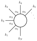
The Wick contraction of a product of such objects consists of terms that are products of Lorentz cycles ${\rm tr}\,(f_{i_{1}}f_{i_{2}}\cdots f_{i_{n}})$ with coefficients that, by suitable IBPs, can be written as integrals of $\tau$ - cycles $\dot{G}_{i_{1}i_{2}}\dot{G}_{i_{2}i_{3}}\cdots\dot{G}_{i_{n}i_{1}}$ . The result can be further simplified by observing that, in the one-dimensional worldline QFT, each factor of

\int_{0}^{T}d\tau_{i_{1}}\cdots\int_{0}^{T}d\tau_{i_{n}}\dot{G}_{i_{1}i_{2}}\dot{G}_{i_{2}i_{3}}\cdots\dot{G}_{i_{n}i_{1}}{\rm tr}\,(f_{i_{1}}f_{i_{2}}\cdots f_{i_{n}})\,,

can be identified with the one-loop $n$ - point Feynman diagram depicted in Fig. 14.

Products of such factors in the worldline theory correspond to disconnected diagrams, and by standard combinatorics can be reduced to the exponential of the sum of all connected diagrams. In this way, and with the usual rescaling $\tau_{i}=Tu_{i}$ , we arrive at

	$\displaystyle\bigl{\langle}V^{\gamma\,({\rm LE})}_{\rm scal}[f_{1}]V^{\gamma\,({\rm LE})}_{\rm scal}[f_{2}]\cdots V^{\gamma\,({\rm LE})}_{\rm scal}[f_{N}]\bigr{\rangle}=i^{N}T^{N}\,\exp\biggl{\{}\sum_{m=1}^{\infty}b_{2m}\sum_{\{i_{1}\ldots i_{2m}\}}Z^{\rm dist}_{2m}(\{i_{1}i_{2}\ldots i_{2m}\})\biggr{\}}\bigg{\|}_{f_{1}\ldots f_{N}}\,,$
			(8.6)

where $Z^{\rm dist}_{k}(\{i_{1}i_{2}\ldots i_{k}\})$ denotes the sum over all distinct Lorentz cycles which can be formed with a given subset of indices, e.g. $Z^{\rm dist}_{4}(\{ijkl\})=Z_{4}(ijkl)+Z_{4}(ijlk)+Z_{4}(ikjl)$ , and $b_{n}$ denotes the basic “bosonic cycle integral”

\displaystyle b_{n}

\displaystyle\equiv

\displaystyle\int_{0}^{1}du_{1}du_{2}\ldots du_{n}\,\dot{G}_{12}\dot{G}_{23}\cdots\dot{G}_{n1}\,.

(8.7)

This integral can be expressed in terms of the Bernoulli numbers ${\cal B}_{n}$ [145]

\displaystyle b_{n}=\qquad\left\{\begin{array}[]{r@{\quad\quad}l}-2^{n}{{\cal B}_{n}\over n!}&\qquad n{\rm\quad even}\,,\\ 0&\qquad n{\rm\quad odd}\,.\\ \end{array}\right.

(8.10)

Eq. (8.6) can be simplified using the combinatorial fact that

\displaystyle{\rm tr}\Bigl{[}(f_{1}+\ldots+f_{N})^{n}\Bigr{]}\bigg{|}_{\rm all\,\,different}

\displaystyle=

\displaystyle 2n\sum_{\{i_{1}\ldots i_{n}\}}Z^{\rm dist}_{n}(\{i_{1}i_{2}\ldots i_{n}\})\,,

( $n\neq 0$ ). Introducing $f_{\rm tot}\equiv\sum_{i=1}^{N}f_{i}$ , using all this in (LABEL:Nphotonvertop) and eliminating the $T$ -integral, we arrive at the following formula for the low-energy limit of the one-loop $N$ -photon amplitude [130]:

\displaystyle\Gamma_{\rm scal}^{({\rm LE})}(k_{1},\varepsilon_{1};\ldots;k_{N},\varepsilon_{N})

\displaystyle=

\displaystyle\frac{e^{N}\Gamma(N-\frac{D}{2})}{(4\pi)^{2}m^{2N-D}}\,\exp\biggl{\{}\sum_{m=1}^{\infty}\frac{b_{2m}}{4m}{\rm tr}\,(f_{\rm tot}^{2m})\biggr{\}}\bigg{|}_{f_{1}\ldots f_{N}}\,.

According to the above, the transition from scalar to spinor QED at this level can be effected by replacing the “chain integral” (8.7) by the “super chain integral”

	$\displaystyle\int_{0}^{1}du_{1}du_{2}\ldots du_{n}\,\Bigl{(}\dot{G}_{12}\dot{G}_{23}\cdots\dot{G}_{n1}-G_{F12}G_{F23}\cdots G_{Fn1}\Bigr{)}=(2-2^{n})\,b_{n}\,.$
			(8.13)

The only other change is a global factor of $(-2)$ for statistics and degrees of freedom. Therefore

\displaystyle\Gamma_{\rm spin}^{({\rm LE})}(k_{1},\varepsilon_{1};\ldots;k_{N},\varepsilon_{N})

\displaystyle=

\displaystyle-2\frac{e^{N}\Gamma(N-\frac{D}{2})}{(4\pi)^{2}m^{2N-d}}\,\exp\biggl{\{}\sum_{m=1}^{\infty}(1-2^{2m-1})\frac{b_{2m}}{2m}{\rm tr}\,(f_{\rm tot}^{2m})\biggr{\}}\bigg{|}_{f_{1}\ldots f_{N}}\,.

In the four-point case this gives (setting now also $D=4$ )

$\displaystyle\Gamma_{\rm scal}(k_{1},\varepsilon_{1};...;k_{4},\varepsilon_{4})$	$\displaystyle=$	$\displaystyle\frac{e^{4}}{(4\pi)^{2}m^{4}}\,\Big{\{}b_{4}[Z_{4}(1234)+Z_{4}(1243)+Z_{4}(1324)]$	(8.15)
		$\displaystyle+b_{2}^{2}[Z_{2}(12)Z_{2}(34)+Z_{2}(13)Z_{2}(24)+Z_{2}(14)Z_{2}(23)]\Big{\}}\,,$	(8.15)
$\displaystyle\Gamma_{\rm spin}(k_{1},\varepsilon_{1};...;k_{4},\varepsilon_{4})$	$\displaystyle=$	$\displaystyle-\frac{2e^{4}}{(4\pi)^{2}m^{4}}\,\Big{\{}-14b_{4}\left[Z_{4}(1234)+Z_{4}(1243)+Z_{4}(1324)\right]$
		$\displaystyle+(-2b_{2})^{2}\left[Z_{2}(12)Z_{2}(34)+Z_{2}(13)Z_{2}(24)+Z_{2}(14)Z_{2}(23)\right]\Big{\}}\,.$

These expressions can also be derived from the effective Lagrangians (1.1) resp. (1.4), see [10, 12, 21].

9 Computational strategy

Our goal in this series of paper is to calculate the four-photon amplitudes fully off-shell, and with any number of the photons taken in the low-energy limit. In the previous chapter we have already settled the case where all photons are low-energy, and by momentum conservation it would not make sense to take three of them low-energy, and the fourth not. This leaves the cases of zero, one or two low-energy photons. Let us thus discuss our general strategy for treating each of these cases starting from the worldline representation. It consists of three elements:

Integrating out a low-energy leg: when a photon leg is taken to be at low energy, the corresponding $u_{i}$ - integral becomes polynomial and can be integrated out. For this purpose, it is not necessary to write the integrand out explicitly, since there are formulas available [140] that will allow us to perform all the integrals that can appear at the four-point level, with the result already written in terms of the worldline Green’s functions between the remaining points. Some examples are

\int_{0}^{1}du_{1}G_{12}=\frac{1}{6}\,,

(9.1)

\int_{0}^{1}du_{1}\dot{G}_{12}=0\,,

(9.2)

\int_{0}^{1}du_{3}G_{13}G_{32}=-\frac{1}{6}G_{12}^{2}+\frac{1}{30}\,,

(9.3)

\int_{0}^{1}du_{3}\dot{G}_{13}G_{32}=-\frac{1}{3}\dot{G}_{12}G_{12}\,,

(9.4)

\int_{0}^{1}du_{3}\dot{G}_{13}\dot{G}_{32}=2G_{12}-\frac{1}{3}\,,

(9.5)

\int_{0}^{1}du_{4}\dot{G}_{41}\dot{G}_{42}\dot{G}_{43}=-\frac{1}{6}(\dot{G}_{12}-\dot{G}_{23})(\dot{G}_{23}-\dot{G}_{31})(\dot{G}_{31}-\dot{G}_{12})\,.

(9.6)

2.

Tensor reduction by IBP: as usual, we are aiming at a reduction to purely scalar integrals, which in the worldline representation means that we wish to remove the polynomial prefactors of the universal exponential $\,{\rm e}^{(\cdot)}$ . Although at the one-loop level there are various ready-made tensor reduction schemes available, to use those we would have to first split the worldline parameter integrals into the ordered sectors to convert them into Feynman-Schwinger parameter integrals. Here, we will rather develop tensor reduction schemes that are adapted to the worldline representation and make it possible to perform the reduction to scalar integrals without the need to fix an ordering for the photon legs.
3.

Tensor reduction by differentiation: any factor of $\dot{G}_{ij}^{2}$ in the integrand can, using the identity $\dot{G}_{ij}^{2}=1-4G_{ij}$ , be generated from the universal exponential through a derivative with respect to $k_{i}\cdot k_{j}$ .

The “two-low” case will involve only integration, while in the “one-low” case integration and tensor reduction will have to be combined. For “zero low” we have a pure tensor reduction task.

The final (dimensionally regularized) scalar integrals will be expressible in terms of hypergeometric functions, namely ${}_{2}F_{1}$ in the two-low case (as for two-point functions), ${}_{2}F_{1}$ and $F_{1}$ in the one-low case (as for three-point functions), and ${}_{2}F_{1}$ , $F_{1}$ and the Lauricella-Saran function for general kinematics (see [146] and refs. therein).

10 Summary and outlook

In this first part of a series of four papers on the (scalar and spinor) QED four-photon amplitudes fully off-shell, our main purpose was to motivate this whole effort, and to prepare the ground for the following parts, where these amplitudes are calculated with general kinematics (part 4), and with one (part 3) or two (part 2) legs taken in the low-energy limit. Thus these sequel papers are all meant to be used together with the present part 1 (although a reader of part 4, for example, would not need to look at part 2 or part 3, if his or her interest is only in the case of general kinematics). The simplest case where all four photons are low energy is a textbook calculation but has been included here for completeness, and as a warm-up demonstrating the efficiency of the formalism which allows one to trivialize this computation even for an arbitrary number of photons.

The main new result of part 1 is a further refinement of the worldline IBP procedure, originally proposed by Bern and Kosower in the gluonic context, and later systematized by Strassler. It leads to an extremely compact integrand for the four-photon amplitudes in both scalar and spinor QED, and at the same time projects these amplitudes, already at the integrand level, into the well-known minimal transversal basis of five tensors proposed by Costantini et al. in 1971. Since the four-photon amplitude is the prototype of all amplitudes with four gauge bosons, we expect this to lead to similar improvements for other cases, such as the form-factor decomposition of the four-gluon amplitudes obtained in [147] using the same formalism.

We have outlined the strategy that we will follow in the calculation of the integrals for the various cases, including the details of the integrating out of a low-energy photon ⁴⁴4In the very recent [148] a similar strategy was followed in the dispersive calculation of the hadronic light-by-light contribution to the muon anomalous magnetic momentum., and derived a set of “matching identities” that will be used in part 4 to facilitate the tensor reduction, but which we include here since they may well turn out to be of more general significance.

Further, we have reviewed the history of photonic processes in general and the four-photon amplitudes in particular, with an emphasis on processes that naturally involve some off-shell photons, either because external fields are involved or we use the amplitude as a building block for a higher-order process. We have also given a summary of the worldline approach to the calculation of such processes.

The improved worldline representation of the four-photon amplitudes developed here offers significant advantages also for the on-shell case. A complete recalculation of the massive scalar and spinor QED on-shell four-photon amplitudes along the present lines is in progress and will be presented in a separate publication.

Acknowledgements: We thank D. Bernard, G. Colangelo, A. Davydychev, H. Gies, F. Karbstein, T. Riemann, K. Scharnhorst and R. Shaisultanov for helpful conversations or correspondence. M. A. Lopez-Lopez is grateful to CoReLS and C.H. Nam for his hospitality during the first stages of this work. C. Lopez-Arcos, M. A. Lopez-Lopez and C. Schubert thank CONACYT for financial support.

Appendix A Conventions

We use natural units $c=\hbar=1$ . We work in euclidean space with a positive definite metric $(g_{\mu\nu})={\rm diag}(++++)$ . Minkowski space amplitudes with metric $(\eta_{\mu\nu})={\rm diag}(-+++)$ are obtained by analytically continuing

$\displaystyle g_{\mu\nu}$	$\displaystyle\rightarrow$	$\displaystyle\eta_{\mu\nu}\,,$
$\displaystyle k^{4}$	$\displaystyle\rightarrow$	$\displaystyle-ik^{0}\,,$
$\displaystyle T$	$\displaystyle\rightarrow$	$\displaystyle is\,.$	(A.1)

We use the absolute value of the electron charge $e=|e|$ , corresponding to a covariant derivative $D_{\mu}=\partial_{\mu}+ieA_{\mu}$ . Momenta of external photons are ingoing.

References

[1] P. A. M. Dirac, R. H. Fowler, The quantum theory of the electron, Proceedings of the Royal Society of London. Series A 117 (778) (1928) 610–624. doi:10.1098/rspa.1928.0023.
URL https://royalsocietypublishing.org/doi/abs/10.1098/rspa.1928.0023
[2] P. A. M. Dirac, Quantised singularities in the electromagnetic field,, Proceedings of the Royal Society of London. Series A 133 (821) (1931) 60–72. doi:10.1098/rspa.1931.0130.
URL https://royalsocietypublishing.org/doi/abs/10.1098/rspa.1931.0130
[3] W. Heisenberg, H. Euler, Consequences of Dirac’s theory of positrons, Z. Phys. 98 (11-12) (1936) 714–732. arXiv:physics/0605038, doi:10.1007/BF01343663.
[4] V. Weisskopf, The electrodynamics of the vacuum based on the quantum theory of the electron, Kong. Dan. Vid. Sel. Mat. Fys. Med. 14N6 (1936) 1–39. doi:10.1017/CBO9780511608223.018.
[5] G. V. Dunne, Heisenberg-euler effective lagrangians: Basics and extensions, in: From Fields to Strings: Circumnavigating Theoretical Physics, 2005, pp. 445–522. arXiv:hep-th/0406216, doi:10.1142/9789812775344_0014.
URL https://www.worldscientific.com/doi/abs/10.1142/9789812775344_0014
[6] H. Euler, B. Kockel, The scattering of light by light in Dirac’s theory, Naturwiss. 23 (15) (1935) 246–247. doi:10.1007/BF01493898.
[7] H. Euler, On the scattering of light by light according to Dirac’s theory, Annalen der Physik 418 (5) (1936) 398–448. doi:10.1002/andp.19364180503.
URL https://onlinelibrary.wiley.com/doi/abs/10.1002/andp.19364180503
[8] A. Akhiezer, L. Landau, I. Pomeranchuk, Scattering of light by light, Nature 138 (3483) (1936) 206. doi:10.1038/138206a0.
[9] A. Achieser, Über die Streuung von Licht an Licht, Phys. Z. Sowjetunion 11 (3) (1937) 263–283.
[10] C. Itzykson, J. Zuber, Quantum Field Theory, International Series In Pure and Applied Physics, McGraw-Hill, New York, 1980.
[11] W. Dittrich, H. Gies, Probing the quantum vacuum. Perturbative effective action approach in quantum electrodynamics and its application, Vol. 166, 2000. doi:10.1007/3-540-45585-X.
[12] V. Berestetskii, E. Lifshitz, L. Pitaevskii, Chapter XII - Radiative Corrections, in: V. Berestetskii, E. Lifshitz, L. Pitaevskii (Eds.), Quantum Electrodynamics, 2nd Edition, Butterworth-Heinemann, Oxford, 1982, pp. 501 – 596. doi:https://doi.org/10.1016/B978-0-08-050346-2.50018-0.
URL http://www.sciencedirect.com/science/article/pii/B9780080503462500180
[13] A. Akhiezer, V. Berestetsky, Quantum electrodynamics, Nauka, Moscow, 1981 (in Russian).
[14] K. Scharnhorst, Photon-photon scattering and related phenomena. Experimental and theoretical approaches: The early periodarXiv:1711.05194.
[15] R. Karplus, M. Neuman, Non-linear interactions between electromagnetic fields, Phys. Rev. 80 (1950) 380–385. doi:10.1103/PhysRev.80.380.
URL https://link.aps.org/doi/10.1103/PhysRev.80.380
[16] R. Karplus, M. Neuman, The scattering of light by light, Phys. Rev. 83 (1951) 776–784. doi:10.1103/PhysRev.83.776.
URL https://link.aps.org/doi/10.1103/PhysRev.83.776
[17] B. De Tollis, Dispersive approach to photon-photon scattering, Nuovo Cim. 32 (3) (1964) 757–768. doi:10.1007/BF02735895.
[18] B. De Tollis, The scattering of photons by photons, Nuovo Cim. 35 (4) (1965) 1182–1193. doi:10.1007/BF02735534.
[19] D. Tommasini, D. Novoa, L. Roso, Quantum vacuum polarization searches with high power lasers below the pair production regime, in: K. Yamanouchi, G. Paulus, D. Mathur (Eds.), Progress in Ultrafast Intense Laser Science, Vol. 106, Springer Series in Chemical Physics, Springer, Cham., 2014, pp. 137–153. doi:10.1007/978-3-319-00521-8_9.
[20] C. Bernicot, J.-P. Guillet, Six-photon amplitudes in scalar QED, Journal of High Energy Physics 2008 (01) (2008) 059. arXiv:0711.4713, doi:10.1088/1126-6708/2008/01/059.
URL https://doi.org/10.1088%2F1126-6708%2F2008%2F01%2F059
[21] L. C. Martin, C. Schubert, V. M. Villanueva, On the low-energy limit of the QED N-photon amplitudes, Nuclear Physics B 668 (1) (2003) 335 – 344. arXiv:hep-th/0301022, doi:https://doi.org/10.1016/S0550-3213(03)00578-9.
URL http://www.sciencedirect.com/science/article/pii/S0550321303005789
[22] J. P. Edwards, A. Huet, C. Schubert, On the low-energy limit of the QED N-photon amplitudes: part 2, Nuclear Physics B 935 (2018) 198 – 209. arXiv:1807.10697, doi:https://doi.org/10.1016/j.nuclphysb.2018.07.026.
URL http://www.sciencedirect.com/science/article/pii/S0550321318302256
[23] Z. Bern, A. D. Freitas, A. Ghinculov, H. Wong, L. Dixon, QCD and QED corrections to light-by-light scattering, Journal of High Energy Physics 11 (11) (2001) 031–031. arXiv:hep-ph/0109079, doi:10.1088/1126-6708/2001/11/031.
URL https://doi.org/10.1088%2F1126-6708%2F2001%2F11%2F031
[24] T. Binoth, E. N. Glover, P. Marquard, J. J. van der Bij, Two-loop corrections to light-by-light scattering in supersymmetric QED, Journal of High Energy Physics 05 (05) (2002) 060–060. arXiv:hep-ph/0202266, doi:10.1088/1126-6708/2002/05/060.
URL https://doi.org/10.1088%2F1126-6708%2F2002%2F05%2F060
[25] G. Jikia, A. Tkabladze, Photon-photon scattering at the photon linear collider, Physics Letters B 323 (3) (1994) 453 – 458. arXiv:hep-ph/9312228, doi:https://doi.org/10.1016/0370-2693(94)91246-7.
URL http://www.sciencedirect.com/science/article/pii/0370269394912467
[26] G. J. Gounaris, P. I. Porfyriadis, F. M. Renard, The $\gamma\gamma\to\gamma\gamma$ process in the standard and SUSY models at high-energies, Eur. Phys. J. C9 (1999) 673–686. arXiv:hep-ph/9902230, doi:10.1007/s100529900079.
[27] V. Costantini, B. De Tollis, G. Pistoni, Nonlinear effects in quantum electrodynamics, Nuovo Cim. A 2 (3) (1971) 733–787. doi:10.1007/BF02736745.
[28] R. A. Leo, A. Minguzzi, G. Soliani, Tensor Amplitudes for Elastic Photon-Photon Scattering, Nuovo Cim. A30 (1975) 270. doi:10.1007/BF02730173.
[29] J. Gervais, A. Neveu, Feynman rules for massive gauge fields with dual diagram topology, Nuclear Physics B 46 (2) (1972) 381 – 401. doi:https://doi.org/10.1016/0550-3213(72)90071-5.
URL http://www.sciencedirect.com/science/article/pii/0550321372900715
[30] Z. Bern, D. A. Kosower, Efficient calculation of one-loop QCD amplitudes, Phys. Rev. Lett. 66 (1991) 1669–1672. doi:10.1103/PhysRevLett.66.1669.
URL https://link.aps.org/doi/10.1103/PhysRevLett.66.1669
[31] Z. Bern, D. C. Dunbar, A mapping between Feynman and string motivated one-loop rules in gauge theories, Nuclear Physics B 379 (3) (1992) 562 – 601. doi:https://doi.org/10.1016/0550-3213(92)90135-X.
URL http://www.sciencedirect.com/science/article/pii/055032139290135X
[32] M. J. Strassler, The Bern-Kosower Rules and Their Relation to Quantum Field Theory, Ph.D. thesis, Stanford University (Jan. 1993).
[33] R. P. Feynman, Mathematical formulation of the quantum theory of electromagnetic interaction, Phys. Rev. 80 (1950) 440–457. doi:10.1103/PhysRev.80.440.
[34] R. P. Feynman, An Operator calculus having applications in quantum electrodynamics, Phys. Rev. 84 (1951) 108–128. doi:10.1103/PhysRev.84.108.
[35] M. J. Strassler, Field theory without feynman diagrams: One-loop effective actions, Nuclear Physics B 385 (1) (1992) 145–184. doi:https://doi.org/10.1016/0550-3213(92)90098-V.
URL https://www.sciencedirect.com/science/article/pii/055032139290098V
[36] C. Schubert, The Structure of the Bern-Kosower integrand for the N gluon amplitude, Eur. Phys. J. C5 (1998) 693–699. arXiv:hep-th/9710067, doi:10.1007/s100520050311,10.1007/s100529800877.
[37] N. Ahmadiniaz, C. Schubert, V. M. Villanueva, String-inspired representations of photon/gluon amplitudes, JHEP 01 (2013) 132. arXiv:1211.1821, doi:10.1007/JHEP01(2013)132.
[38] D. Bernard, F. Moulin, F. Amiranoff, A. Braun, J. Chambaret, G. Darpentigny, G. Grillon, S. Ranc, F. Perrone, Search for stimulated photon-photon scattering in vacuum, The European Physical Journal D 10 (1) (2000) 141–145. arXiv:1007.0104, doi:10.1007/s100530050535.
URL http://dx.doi.org/10.1007/s100530050535
[39] D. Bernard, G. Brodin, M. Marklund, Elastic Photon-Photon Scattering: A Test Bench for ELI’s Design Study, (Written version of the talk presented by D. Bernard at the workshop) High Field Physics ELI Workshop, Garching, Nov. 13 - 14, 2006.
[40] J. Lundin, M. Marklund, E. Lundström, G. Brodin, J. Collier, R. Bingham, J. T. Mendonça, P. Norreys, Analysis of four-wave mixing of high-power lasers for the detection of elastic photon-photon scattering, Phys. Rev. A 74 (2006) 043821. arXiv:hep-ph/0606136, doi:10.1103/PhysRevA.74.043821.
URL https://link.aps.org/doi/10.1103/PhysRevA.74.043821
[41] D. Tommasini, A. Ferrando, H. Michinel, M. Seco, Precision tests of QED and non-standard models by searching photon-photon scattering in vacuum with high power lasers, Journal of High Energy Physics 11 (11) (2009) 043–043. arXiv:0909.4663, doi:10.1088/1126-6708/2009/11/043.
URL https://doi.org/10.1088%2F1126-6708%2F2009%2F11%2F043
[42] H. Gies, F. Karbstein, C. Kohlfürst, All-optical signatures of strong-field qed in the vacuum emission picture, Phys. Rev. D 97 (2018) 036022. arXiv:1712.03232, doi:10.1103/PhysRevD.97.036022.
URL https://link.aps.org/doi/10.1103/PhysRevD.97.036022
[43] H. Gies, F. Karbstein, C. Kohlfürst, N. Seegert, Photon-photon scattering at the high-intensity frontier, Phys. Rev. D 97 (2018) 076002. arXiv:1712.06450, doi:10.1103/PhysRevD.97.076002.
URL https://link.aps.org/doi/10.1103/PhysRevD.97.076002
[44] F. Moulin, D. Bernard, Four-wave interaction in gas and vacuum. Definition of a third order nonlinear effective susceptibility in vacuum: $\chi_{vacuum^{(3)}}$ , Opt. Commun. 164 (1999) 137–144. arXiv:physics/0203069, doi:10.1016/S0030-4018(99)00169-8.
[45] H. Gies, F. Karbstein, L. Klar, All-optical quantum vacuum signals in two-beam collisions, Phys. Rev. D 106 (2022) 116005. doi:10.1103/PhysRevD.106.116005.
URL https://link.aps.org/doi/10.1103/PhysRevD.106.116005
[46] H. Gies, F. Karbstein, L. Klar, Quantum vacuum signatures in multicolor laser pulse collisions, Phys. Rev. D 103 (2021) 076009. doi:10.1103/PhysRevD.103.076009.
URL https://link.aps.org/doi/10.1103/PhysRevD.103.076009
[47] A. Fedotov, A. Ilderton, F. Karbstein, B. King, D. Seipt, H. Taya, G. Torgrimsson, Advances in QED with intense background fields, Phys. Rept. 1010 (2023) 1–138. arXiv:2203.00019, doi:10.1016/j.physrep.2023.01.003.
[48] M. Aaboud, et al., Evidence for light-by-light scattering in heavy-ion collisions with the ATLAS detector at the LHC, Nature Physics 13 (9) (2017) 852–858. arXiv:1702.01625, doi:10.1038/nphys4208.
URL http://dx.doi.org/10.1038/nphys4208
[49] M. Vysotsky, E. Zhemchugov, LHC as a photon-photon collider, in: 25th Rencontres du Vietnam: Windows on the Universe, 2018. arXiv:1812.02493.
[50] A. M. Sirunyan, et al., Evidence for light-by-light scattering and searches for axion-like particles in ultraperipheral PbPb collisions at $\sqrt{s_{\mathrm{NN}}}=5.02$ TeV, Phys. Lett. B 797 (2019) 134826. arXiv:1810.04602, doi:10.1016/j.physletb.2019.134826.
[51] G. Aad, et al., Observation of light-by-light scattering in ultraperipheral Pb+Pb collisions with the ATLAS detector, Phys. Rev. Lett. 123 (5) (2019) 052001. arXiv:1904.03536, doi:10.1103/PhysRevLett.123.052001.
[52] L. Schoeffel, C. Baldenegro, H. Hamdaoui, S. Hassani, C. Royon, M. Saimpert, Photon–photon physics at the LHC and laser beam experiments, present and future, Prog. Part. Nucl. Phys. 120 (2021) 103889. arXiv:2010.07855, doi:10.1016/j.ppnp.2021.103889.
[53] G. K. Krintiras, I. Grabowska-Bold, M. Kłusek-Gawenda, E. Chapon, R. Chudasama, R. Granier de Cassagnac, Light-by-light scattering cross-section measurements at LHCarXiv:2204.02845.
[54] D. d’Enterria, G. G. da Silveira, Observing Light-by-Light Scattering at the Large Hadron Collider, Phys. Rev. Lett. 111 (2013) 080405. arXiv:1305.7142, doi:10.1103/PhysRevLett.111.080405.
URL https://link.aps.org/doi/10.1103/PhysRevLett.111.080405
[55] M. Kłusek-Gawenda, P. Lebiedowicz, A. Szczurek, Light-by-light scattering in ultraperipheral Pb-Pb collisions at energies available at the CERN Large Hadron Collider, Phys. Rev. C 93 (2016) 044907. arXiv:1601.07001, doi:10.1103/PhysRevC.93.044907.
URL https://link.aps.org/doi/10.1103/PhysRevC.93.044907
[56] J. Ellis, N. E. Mavromatos, P. Roloff, T. You, Light-by-light scattering at future $e^{+}e^{-}$ colliders, Eur. Phys. J. C 82 (7) (2022) 634. arXiv:2203.17111, doi:10.1140/epjc/s10052-022-10565-w.
[57] F. Sauter, Über das Verhalten eines Elektrons im homogenen elektrischen Feld nach der relativistischen Theorie Diracs, Zeitschrift für Physik 69 (11-12) (1931) 742–764. doi:10.1007/BF01339461.
[58] M. Born, L. Infeld, Foundations of the new field theory, Proc. Roy. Soc. Lond. A 144 (852) (1934) 425–451. doi:10.1098/rspa.1934.0059.
[59] M. A. Trejo, Cotas fenomenológicas para el parámetro libre de la teoría Born-Infeld, Master’s thesis, IFM, UMSNH (2011).
URL http://bibliotecavirtual.dgb.umich.mx:8083/xmlui/handle/DGB_UMICH/1158
[60] J. M. Davila, C. Schubert, M. A. Trejo, Photonic processes in Born-Infeld theory[Int. J. Mod. Phys.A29,1450174(2014)]. arXiv:1310.8410, doi:10.1142/S0217751X14501747.
[61] J. Ellis, N. E. Mavromatos, T. You, Light-by-Light Scattering Constraint on Born-Infeld Theory, Phys. Rev. Lett. 118 (2017) 261802. arXiv:1703.08450, doi:10.1103/PhysRevLett.118.261802.
URL https://link.aps.org/doi/10.1103/PhysRevLett.118.261802
[62] T. Inada, T. Yamazaki, T. Yamaji, Y. Seino, X. Fan, S. Kamioka, T. Namba, S. Asai, Probing Physics in Vacuum Using an X-ray Free-Electron Laser, a High-Power Laser, and a High-Field Magnet, Science 7 (2017) 671. arXiv:1707.00253, doi:10.3390/app7070671.
[63] S. Shakeri, D. J. E. Marsh, S.-S. Xue, Light by Light Scattering as a New Probe for AxionsarXiv:2002.06123.
[64] S. C. İnan, A. V. Kisselev, Polarized light-by-light scattering at the CLIC induced by axion-like particles, Chin. Phys. C 45 (4) (2021) 043109. arXiv:2007.01693, doi:10.1088/1674-1137/abe0be.
[65] B. Badelek, C. Blochinger, J. Blumlein, E. Boos, R. Brinkmann, H. Burkhardt, P. Bussey, C. Carimalo, J. Chyla, A. K. Ciftci, W. Decking, A. D. Roeck, V. Fadin, M. Ferrario, A. Finch, H. Fraas, F. Franke, M. Galynskii, A. Gamp, I. Ginzburg, R. Godbole, D. S. Gorbunov, G. Gounaris, K. Hagiwara, L. Han, R. D. Heuer, C. Heusch, J. Illana, V. Ilyin, P. Jankowski, Y. Jiang, G. Jikia, L. Jonsson, M. Kalachnikow, F. Kapusta, R. Klanner, M. Klasen, K. Kobayashi, T. Kon, G. Kotkin, M. Kramer, M. Krawczyk, Y. P. Kuang, E. Kuraev, J. Kwiecinski, M. Leenen, M. Levchuk, W. F. Ma, H. Martyn, T. Mayer, M. Melles, D. J. Miller, S. Mtingwa, M. Muhlleitner, B. Muryn, P. V. Nickles, R. Orava, G. Pancheri, A. Penin, A. Potylitsyn, P. Poulose, T. Quast, P. Raimondi, H. Redlin, F. Richard, S. D. Rindani, T. Rizzo, E. Saldin, W. Sandner, H. Schonnagel, E. Schneidmiller, H. J. Schreiber, S. Schreiber, K. P. Schuler, V. Serbo, A. Seryi, R. Shanidze, W. D. Silva, S. Soldner-Rembold, M. Spira, A. M. Stasto, S. Sultansoy, T. Takahashi, V. Telnov, A. Tkabladze, D. Trines, A. Undrus, A. Wagner, N. Walker, I. Watanabe, T. Wengler, I. Will, S. Wipf, O. Yavas, K. Yokoya, M. Yurkov, A. F. Zarnecki, P. Zerwas, F. Zomer, The photon collider at tesla, International Journal of Modern Physics A 19 (30) (2004) 5097–5186. arXiv:hep-ex/0108012, doi:10.1142/S0217751X04020737.
URL https://doi.org/10.1142/S0217751X04020737
[66] T. Takahashi, G. An, Y. Chen, W. Chou, Y. Huang, W. Liu, W. Lu, J. Lv, G. Pei, S. Pei, et al., Light-by-light scattering in a photon-photon collider, The European Physical Journal C 78 (11) (2018) 893. arXiv:1807.00101, doi:10.1140/epjc/s10052-018-6364-1.
URL http://dx.doi.org/10.1140/epjc/s10052-018-6364-1
[67] V. I. Telnov, Gamma-gamma collider with $W_{\gamma\gamma}\leq$ 12 GeV based on the 17.5 GeV SC linac of the European XFEL, JINST 15 (10) (2020) P10028. arXiv:2007.14003, doi:10.1088/1748-0221/15/10/P10028.
[68] M. Sangal, C. H. Keitel, M. Tamburini, Observing light-by-light scattering in vacuum with an asymmetric photon collider, Phys. Rev. D 104 (2021) L111101. doi:10.1103/PhysRevD.104.L111101.
URL https://link.aps.org/doi/10.1103/PhysRevD.104.L111101
[69] D. Hanneke, S. Fogwell, G. Gabrielse, New measurement of the electron magnetic moment and the fine structure constant, Phys. Rev. Lett. 100 (2008) 120801. arXiv:0801.1134, doi:10.1103/PhysRevLett.100.120801.
URL https://link.aps.org/doi/10.1103/PhysRevLett.100.120801
[70] G. W. Bennett, B. Bousquet, H. N. Brown, G. Bunce, R. M. Carey, P. Cushman, G. T. Danby, P. T. Debevec, M. Deile, H. Deng, W. Deninger, S. K. Dhawan, V. P. Druzhinin, L. Duong, E. Efstathiadis, F. J. M. Farley, G. V. Fedotovich, S. Giron, F. E. Gray, D. Grigoriev, M. Grosse-Perdekamp, A. Grossmann, M. F. Hare, D. W. Hertzog, X. Huang, V. W. Hughes, M. Iwasaki, K. Jungmann, D. Kawall, M. Kawamura, B. I. Khazin, J. Kindem, F. Krienen, I. Kronkvist, A. Lam, R. Larsen, Y. Y. Lee, I. Logashenko, R. McNabb, W. Meng, J. Mi, J. P. Miller, Y. Mizumachi, W. M. Morse, D. Nikas, C. J. G. Onderwater, Y. Orlov, C. S. Özben, J. M. Paley, Q. Peng, C. C. Polly, J. Pretz, R. Prigl, G. zu Putlitz, T. Qian, S. I. Redin, O. Rind, B. L. Roberts, N. Ryskulov, S. Sedykh, Y. K. Semertzidis, P. Shagin, Y. M. Shatunov, E. P. Sichtermann, E. Solodov, M. Sossong, A. Steinmetz, L. R. Sulak, C. Timmermans, A. Trofimov, D. Urner, P. von Walter, D. Warburton, D. Winn, A. Yamamoto, D. Zimmerman, Final report of the E821 muon anomalous magnetic moment measurement at BNL, Phys. Rev. D 73 (2006) 072003. arXiv:hep-ex/0602035, doi:10.1103/PhysRevD.73.072003.
URL https://link.aps.org/doi/10.1103/PhysRevD.73.072003
[71] H. Cheng, T. T. Wu, Photon-photon scattering close to the forward direction, Phys. Rev. D1 (1970) 3414–3415. doi:10.1103/PhysRevD.1.3414.
[72] W. Dittrich, Relativistic Eikonal Physics, Fortsch. Phys. 22 (1974) 539–574. doi:10.1002/prop.19740221002.
[73] A. Czarnecki, R. Szafron, Light-by-light scattering in the Lamb shift and the bound electron g factor, Phys. Rev. A94 (6) (2016) 060501. arXiv:1611.04875, doi:10.1103/PhysRevA.94.060501.
[74] A. Czarnecki, J. Piclum, R. Szafron, Logarithmically enhanced Euler-Heisenberg Lagrangian contribution to the electron gyromagnetic factor, Phys. Rev. A102 (5) (2020) 050801. arXiv:2008.07550, doi:10.1103/PhysRevA.102.050801.
[75] G. S. Adkins, C. Parsons, M. D. Salinger, R. Wang, R. N. Fell, Positronium energy levels at order $m\alpha^{7}$ : light-by-light scattering in the two-photon-annihilation channel, Phys. Rev. A90 (4) (2014) 042502. arXiv:1407.8232, doi:10.1103/PhysRevA.90.042502.
[76] R. R. Wilson, Scattering of ${1.3}^{3}$ Mev Gamma-Rays by an Electric Field, Phys. Rev. 90 (1953) 720–721. doi:10.1103/PhysRev.90.720.
URL https://link.aps.org/doi/10.1103/PhysRev.90.720
[77] M. Schumacher, I. Borchert, F. Smend, P. Rullhusen, Delbrück scattering of $2.75$ MeV photons by lead, Physics Letters B 59 (2) (1975) 134 – 136. doi:https://doi.org/10.1016/0370-2693(75)90685-1.
URL http://www.sciencedirect.com/science/article/pii/0370269375906851
[78] T. Bar-Noy, S. Kahane, Numerical calculations of Delbrück scattering amplitudes, Nuclear Physics A 288 (1) (1977) 132 – 140. doi:https://doi.org/10.1016/0375-9474(77)90084-7.
URL http://www.sciencedirect.com/science/article/pii/0375947477900847
[79] B. Fornal, Is There a Sign of New Physics in Beryllium Transitions?, Int. J. Mod. Phys. A32 (2017) 1730020. arXiv:1707.09749, doi:10.1142/S0217751X17300204.
[80] B. Koch, X17: A new force, or evidence for a hard $\gamma+\gamma$ process?, Nucl. Phys. A 1008 (2021) 122143. arXiv:2003.05722, doi:10.1016/j.nuclphysa.2021.122143.
[81] Y. Shima, Photon splitting in a nuclear electric field, Phys. Rev. 142 (1966) 944–956. doi:10.1103/PhysRev.142.944.
URL https://link.aps.org/doi/10.1103/PhysRev.142.944
[82] S. Z. Akhmadaliev, G. Y. Kezerashvili, S. G. Klimenko, R. N. Lee, V. M. Malyshev, A. L. Maslennikov, A. M. Milov, A. I. Milstein, N. Y. Muchnoi, A. I. Naumenkov, V. S. Panin, S. V. Peleganchuk, G. E. Pospelov, I. Y. Protopopov, L. V. Romanov, A. G. Shamov, D. N. Shatilov, E. A. Simonov, V. M. Strakhovenko, Y. A. Tikhonov, Experimental investigation of high-energy photon splitting in atomic fields, Phys. Rev. Lett. 89 (2002) 061802. arXiv:hep-ex/0111084, doi:10.1103/PhysRevLett.89.061802.
URL https://link.aps.org/doi/10.1103/PhysRevLett.89.061802
[83] A. Di Piazza, K. Z. Hatsagortsyan, C. H. Keitel, Non-perturbative vacuum-polarization effects in proton-laser collisions, Phys. Rev. Lett. 100 (2008) 010403. arXiv:0708.0475, doi:10.1103/PhysRevLett.100.010403.
[84] A. Di Piazza, K. Z. Hatsagortsyan, C. H. Keitel, Laser photon merging in proton-laser collisions, Phys. Rev. A78 (2008) 062109. arXiv:0906.5576, doi:10.1103/PhysRevA.78.062109.
[85] J. S. Toll, The Dispersion relation for light and its application to problems involving electron pairs, Ph.D. thesis, Princeton U. (1952).
[86] R. Baier, P. Breitenlohner, The Vacuum refraction Index in the presence of External Fields, Nuovo Cim. B 47 (1967) 117–120. doi:10.1007/BF02712312.
[87] R. Baier, P. Breitenlohner, Photon Propagation in External Fields, Acta Phys. Austriaca 25 (1967) 212–223.
[88] S. L. Adler, Photon splitting and photon dispersion in a strong magnetic field, Annals of Physics 67 (2) (1971) 599 – 647. doi:https://doi.org/10.1016/0003-4916(71)90154-0.
URL http://www.sciencedirect.com/science/article/pii/0003491671901540
[89] W. Dittrich, H. Gies, Vacuum birefringence in strong magnetic fields, in: Workshop on Frontier Tests of Quantum Electrodynamics and Physics of the Vacuum, 1998, pp. 29–43. arXiv:hep-ph/9806417.
[90] J. S. Heyl, L. Hernquist, Birefringence and dichroism of the QED vacuum, Journal of Physics A: Mathematical and General 30 (18) (1997) 6485–6492. arXiv:hep-ph/9705367, doi:10.1088/0305-4470/30/18/022.
URL https://doi.org/10.1088%2F0305-4470%2F30%2F18%2F022
[91] R. Battesti, et al., High magnetic fields for fundamental physics, Phys. Rept. 765-766 (2018) 1–39. arXiv:1803.07547, doi:10.1016/j.physrep.2018.07.005.
[92] R. Cameron, G. Cantatore, A. C. Melissinos, G. Ruoso, Y. Semertzidis, H. J. Halama, D. M. Lazarus, A. G. Prodell, F. Nezrick, C. Rizzo, E. Zavattini, Search for nearly massless, weakly coupled particles by optical techniques, Phys. Rev. D 47 (1993) 3707–3725. doi:10.1103/PhysRevD.47.3707.
URL https://link.aps.org/doi/10.1103/PhysRevD.47.3707
[93] D. Bakalov, F. Brandi, G. Cantatore, G. Carugno, S. Carusotto, F. Della Valle, A. Riva, U. Gastaldi, E. Iacopini, P. Micossi, E. Milotti, R. Onofrio, R. Pengo, F. Perrone, G. Petrucci, E. Polacco, C. Rizzo, G. Ruoso, E. Zavattini, G. Zavattini, The measurement of vacuum polarization: The PVLAS experiment, Hyperfine Interactions 114 (1998) 103–113. doi:10.1023/A:1012610102642.
[94] F. Della Valle, E. Milotti, A. Ejlli, G. Messineo, L. Piemontese, G. Zavattini, U. Gastaldi, R. Pengo, G. Ruoso, First results from the new PVLAS apparatus: A new limit on vacuum magnetic birefringence, Phys. Rev. D 90 (2014) 092003. arXiv:1406.6518, doi:10.1103/PhysRevD.90.092003.
URL https://link.aps.org/doi/10.1103/PhysRevD.90.092003
[95] A. Ejlli, F. Della Valle, U. Gastaldi, G. Messineo, R. Pengo, G. Ruoso, G. Zavattini, The PVLAS experiment: A 25 year effort to measure vacuum magnetic birefringence, Phys. Rept. 871 (2020) 1–74. arXiv:2005.12913, doi:10.1016/j.physrep.2020.06.001.
[96] T. Heinzl, B. Liesfeld, K.-U. Amthor, H. Schwoerer, R. Sauerbrey, A. Wipf, On the observation of vacuum birefringence, Opt. Commun. 267 (2006) 318–321. arXiv:hep-ph/0601076, doi:10.1016/j.optcom.2006.06.053.
[97] B. King, H. Hu, B. Shen, Three-pulse photon-photon scattering, Phys. Rev. A 98 (2) (2018) 023817. arXiv:1805.03688, doi:10.1103/PhysRevA.98.023817.
[98] F. Karbstein, C. Sundqvist, K. S. Schulze, I. Uschmann, H. Gies, G. G. Paulus, Vacuum birefringence at x-ray free-electron lasers, New J. Phys. 23 (9) (2021) 095001. arXiv:2105.13869, doi:10.1088/1367-2630/ac1df4.
[99] F. Karbstein, D. Ullmann, E. A. Mosman, M. Zepf, Direct Accessibility of the Fundamental Constants Governing Light-by-Light Scattering, Phys. Rev. Lett. 129 (6) (2022) 061802. arXiv:2207.09866, doi:10.1103/PhysRevLett.129.061802.
[100] N. Ahmadiniaz, T. E. Cowan, J. Grenzer, S. Franchino-Viñas, A. L. Garcia, M. Šmíd, T. Toncian, M. A. Trejo, R. Schützhold, Detection schemes for quantum vacuum diffraction and birefringencearXiv:2208.14215.
[101] K. Hu, M. G. Baring, Z. Wadiasingh, A. K. Harding, Opacities for Photon Splitting and Pair Creation in Neutron Star Magnetospheres, Mon. Not. Roy. Astron. Soc. 486 (3) (2019) 3327–3349. arXiv:1904.03315, doi:10.1093/mnras/stz995.
[102] H. Gies, F. Karbstein, R. Shaisultanov, Laser photon merging in an electromagnetic field inhomogeneity, Phys. Rev. D 90 (3) (2014) 033007. arXiv:1406.2972, doi:10.1103/PhysRevD.90.033007.
[103] H. Gies, F. Karbstein, N. Seegert, Photon merging and splitting in electromagnetic field inhomogeneities, Phys. Rev. D93 (8) (2016) 085034. arXiv:1603.00314, doi:10.1103/PhysRevD.93.085034.
[104] S. Laporta, E. Remiddi, The Analytical value of the electron light-light graphs contribution to the muon (g-2) in QED, Phys. Lett. B 301 (1993) 440–446. doi:10.1016/0370-2693(93)91176-N.
[105] S. Laporta, High-precision calculation of the 4-loop contribution to the electron g-2 in QED, Phys. Lett. B 772 (2017) 232–238. arXiv:1704.06996, doi:10.1016/j.physletb.2017.06.056.
[106] T. Aoyama, T. Kinoshita, M. Nio, Theory of the Anomalous Magnetic Moment of the Electron, Atoms 7 (1) (2019) 28. doi:10.3390/atoms7010028.
[107] N. Ahmadiniaz, M. Bussmann, T. E. Cowan, A. Debus, T. Kluge, R. Schützhold, Observability of Coulomb-assisted quantum vacuum birefringence, Phys. Rev. D 104 (1) (2021) L011902. arXiv:2012.04484, doi:10.1103/PhysRevD.104.L011902.
[108] N. Ahmadiniaz, T. E. Cowan, M. Ding, M. A. L. Lopez, R. Sauerbrey, R. Shaisultanov, R. Schützhold, Field-assisted birefringent Compton scatteringarXiv:2212.03350.
[109] G. Colangelo, M. Hoferichter, M. Procura, P. Stoffer, Dispersive approach to hadronic light-by-light scattering, JHEP 09 (2014) 091. arXiv:1402.7081, doi:10.1007/JHEP09(2014)091.
[110] J. Bijnens, N. Hermansson-Truedsson, L. Laub, A. Rodríguez-Sánchez, Short-distance HLbL contributions to the muon anomalous magnetic moment beyond perturbation theory, JHEP 10 (2020) 203. arXiv:2008.13487, doi:10.1007/JHEP10(2020)203.
[111] J. Bijnens, N. Hermansson-Truedsson, L. Laub, A. Rodriguez-Sanchez, Short-distance HLbL contributions to the muon g-2, Vol. 312-317, 2021, pp. 180–184. arXiv:2011.12123, doi:10.1016/j.nuclphysbps.2021.05.048.
[112] J. Bijnens, N. Hermansson-Truedsson, A. Rodríguez-Sánchez, Short-distance constraints on the hadronic light-by-light, EPJ Web Conf. 274 (2022) 06010. arXiv:2211.04068, doi:10.1051/epjconf/202227406010.
[113] A. Tarasov, R. Venugopalan, Role of the chiral anomaly in polarized deeply inelastic scattering: Finding the triangle graph inside the box diagram in Bjorken and Regge asymptotics, Phys. Rev. D 102 (11) (2020) 114022. arXiv:2008.08104, doi:10.1103/PhysRevD.102.114022.
[114] A. Abada, J. Matias, R. Pittau, Inelastic photon neutrino interactions using an effective Lagrangian, Phys. Rev. D59 (1999) 013008. arXiv:hep-ph/9806383, doi:10.1103/PhysRevD.59.013008.
[115] S. C. İnan, A. V. Kisselev, Probing anomalous $\gamma\gamma\gamma Z$ couplings through $\gamma Z$ production in $\gamma\gamma$ collisions at the CLIC, JHEP 10 (2021) 121. arXiv:2108.04478, doi:10.1007/JHEP10(2021)121.
[116] A. Abada, J. Matias, R. Pittau, Low-energy photon neutrino inelastic processes beyond the standard model, Phys. Lett. B450 (1999) 173–181. arXiv:hep-ph/9812238, doi:10.1016/S0370-2693(99)00125-2.
[117] H. Gies, J. Jaeckel, A. Ringwald, Polarized light propagating in a magnetic field as a probe for millicharged fermions, Phys. Rev. Lett. 97 (2006) 140402. doi:10.1103/PhysRevLett.97.140402.
URL https://link.aps.org/doi/10.1103/PhysRevLett.97.140402
[118] X. Wong, Y. Huang, Dark photon production via $\gamma\gamma\rightarrow\gamma A^{\prime}$ , Eur. Phys. J. C 81 (5) (2021) 442. arXiv:2103.15079, doi:10.1140/epjc/s10052-021-09228-z.
[119] E. Fradkin, Application of functional methods in quantum field theory and quantum statistics (II), Nucl. Phys. 76 (3) (1966) 588–624. doi:10.1016/0029-5582(66)90200-8.
[120] H. Gies, J. Hammerling, Geometry of spin-field coupling on the worldline, Phys. Rev. D72 (2005) 065018. arXiv:hep-th/0505072, doi:10.1103/PhysRevD.72.065018.
[121] J. P. Edwards, C. Schubert, N-photon amplitudes in a plane-wave background, Phys. Lett. B 822 (2021) 136696. arXiv:2105.08173, doi:10.1016/j.physletb.2021.136696.
[122] R. Shaisultanov, On the string-inspired approach to QED in external field, Physics Letters B 378 (1) (1996) 354 – 356. doi:https://doi.org/10.1016/0370-2693(96)00359-0.
URL http://www.sciencedirect.com/science/article/pii/0370269396003590
[123] M. Reuter, M. G. Schmidt, C. Schubert, Constant external fields in gauge theory and the spin 0, $1/2$ , 1 path integrals, Annals of Physics 259 (2) (1997) 313 – 365. arXiv:hep-th/9610191, doi:https://doi.org/10.1006/aphy.1997.5716.
URL http://www.sciencedirect.com/science/article/pii/S000349169795716X
[124] K. Daikouji, M. Shino, Y. Sumino, Bern-kosower rule for scalar qed, Physical Review D 53 (8) (1996) 4598.
[125] N. Ahmadiniaz, A. Bashir, C. Schubert, Multiphoton amplitudes and generalized Landau-Khalatnikov-Fradkin transformation in scalar QED, Phys. Rev. D 93 (4) (2016) 045023. arXiv:1511.05087, doi:10.1103/PhysRevD.93.045023.
[126] A. Ahmad, N. Ahmadiniaz, O. Corradini, S. P. Kim, C. Schubert, Master formulas for the dressed scalar propagator in a constant field, Nuclear Physics B 919 (2017) 9 – 24. arXiv:1612.02944, doi:https://doi.org/10.1016/j.nuclphysb.2017.03.007.
URL http://www.sciencedirect.com/science/article/pii/S0550321317300871
[127] N. Ahmadiniaz, V. Banda Guzmán, F. Bastianelli, O. Corradini, J. Edwards, C. Schubert, Worldline master formulas for the dressed electron propagator. Part I. Off-shell amplitudes, JHEP 08 (08) (2020) 049. arXiv:2004.01391, doi:10.1007/JHEP08(2020)018.
[128] M. G. Schmidt, C. Schubert, Multiloop calculations in the string-inspired formalism: The single spinor loop in QED, Phys. Rev. D 53 (1996) 2150–2159. doi:10.1103/PhysRevD.53.2150.
URL https://link.aps.org/doi/10.1103/PhysRevD.53.2150
[129] D. Fliegner, M. Reuter, M. Schmidt, C. Schubert, The Two loop Euler-Heisenberg Lagrangian in dimensional renormalization, Theor. Math. Phys. 113 (1997) 1442–1451. arXiv:hep-th/9704194, doi:10.1007/BF02634170.
[130] G. V. Dunne, C. Schubert, Two-loop self-dual Euler-Heisenberg Lagrangians (I): Real part and helicity amplitudes, Journal of High Energy Physics 08 (08) (2002) 053–053. arXiv:hep-th/0205004, doi:10.1088/1126-6708/2002/08/053.
URL https://doi.org/10.1088%2F1126-6708%2F2002%2F08%2F053
[131] G. V. Dunne, C. Schubert, Two loop selfdual Euler-Heisenberg Lagrangians. 2. Imaginary part and Borel analysis, JHEP 06 (2002) 042. arXiv:hep-th/0205005, doi:10.1088/1126-6708/2002/06/042.
[132] I. Huet, D. McKeon, C. Schubert, Euler-Heisenberg lagrangians and asymptotic analysis in 1+1 QED, part 1: Two-loop, JHEP 12 (2010) 036. arXiv:1010.5315, doi:10.1007/JHEP12(2010)036.
[133] I. Huet, M. Rausch De Traubenberg, C. Schubert, Three-loop Euler-Heisenberg Lagrangian in 1 $+$ 1 QED, part 1: single fermion-loop part, JHEP 03 (2019) 167. arXiv:1812.08380, doi:10.1007/JHEP03(2019)167.
[134] J. Nicasio, J. P. Edwards, C. Schubert, N. Ahmadiniaz, Non-perturbative gauge transformations of arbitrary fermion correlation functions in quantum electrodynamicsarXiv:2010.04160.
[135] Z. Bern, D. A. Kosower, The computation of loop amplitudes in gauge theories, Nuclear Physics B 379 (3) (1992) 451 – 561. doi:https://doi.org/10.1016/0550-3213(92)90134-W.
URL http://www.sciencedirect.com/science/article/pii/055032139290134W
[136] Z. Bern, L. Dixon, D. A. Kosower, One-loop corrections to five-gluon amplitudes, Phys. Rev. Lett. 70 (1993) 2677–2680. doi:10.1103/PhysRevLett.70.2677.
URL https://link.aps.org/doi/10.1103/PhysRevLett.70.2677
[137] F. Bastianelli, A. Zirotti, Worldline formalism in a gravitational background, Nuclear Physics B 642 (1) (2002) 372 – 388. doi:https://doi.org/10.1016/S0550-3213(02)00683-1.
URL http://www.sciencedirect.com/science/article/pii/S0550321302006831
[138] F. Bastianelli, O. Corradini, A. Zirotti, Dimensional regularization for $\mathcal{N}=1$ supersymmetric sigma models and the worldline formalism, Phys. Rev. D 67 (2003) 104009. arXiv:hep-th/0211134, doi:10.1103/PhysRevD.67.104009.
URL https://link.aps.org/doi/10.1103/PhysRevD.67.104009
[139] N. Ahmadiniaz, F. M. Balli, O. Corradini, J. M. Dávila, C. Schubert, Compton-like scattering of a scalar particle with n photons and one graviton, Nuclear Physics B 950 (2020) 114877. doi:https://doi.org/10.1016/j.nuclphysb.2019.114877.
URL http://www.sciencedirect.com/science/article/pii/S0550321319303633
[140] C. Schubert, Perturbative quantum field theory in the string-inspired formalism, Physics Reports 355 (2) (2001) 73 – 234. arXiv:hep-th/0101036, doi:https://doi.org/10.1016/S0370-1573(01)00013-8.
URL http://www.sciencedirect.com/science/article/pii/S0370157301000138
[141] N. Ahmadiniaz, F. M. Balli, C. Lopez-Arcos, A. Q. Velez, C. Schubert, Color-kinematics duality from the Bern-Kosower formalism, Phys. Rev. D 104 (4) (2021) L041702. arXiv:2105.06745, doi:10.1103/PhysRevD.104.L041702.
[142] Z. Bern, J. J. M. Carrasco, H. Johansson, New Relations for Gauge-Theory Amplitudes, Phys. Rev. D 78 (2008) 085011. arXiv:0805.3993, doi:10.1103/PhysRevD.78.085011.
[143] A. Polyakov, Gauge Fields and Strings, Contemporary Concepts in Physics, Harwood Academic Publishers, 1987.
URL http://books.google.it/books?id=uaI8xcjJ8LMC
[144] Y. Liang, A. Czarnecki, Photon-photon scattering: A Tutorial, Can. J. Phys. 90 (2012) 11–26. arXiv:1111.6126, doi:10.1139/p11-144.
[145] M. G. Schmidt, C. Schubert, On the calculation of effective actions by string methods, Physics Letters B 318 (3) (1993) 438 – 446. doi:https://doi.org/10.1016/0370-2693(93)91537-W.
URL http://www.sciencedirect.com/science/article/pii/037026939391537W
[146] T. Riemann, J. Usovitsch, Scalar 1-loop Feynman integrals in arbitrary space-time dimension $d$ - an update, CERN Yellow Reports: Monographs 3 (2020) 139–162. doi:10.23731/CYRM-2020-003.139.
[147] N. Ahmadiniaz, C. Schubert, QCD gluon vertices from the string-inspired formalism, International Journal of Modern Physics E 25 (07) (2016) 1642004. arXiv:1811.10780, doi:10.1142/S0218301316420040.
URL https://doi.org/10.1142/S0218301316420040
[148] J. Lüdtke, M. Procura, P. Stoffer, Dispersion relations for hadronic light-by-light scattering in triangle kinematicsarXiv:2302.12264.

The QED four – photon amplitudes off-shell: part 1

Abstract

1 Introduction: Photon amplitudes in QED

2 Phenomenological uses of the QED four-photon amplitude

2.1 Pure QED

2.1.1 Purely photonic processes

2.1.2 Photonic processes involving Coulomb fields

2.1.3 Photonic processes involving magnetic fields

2.1.4 Photonic processes involving Coulomb and magnetic fields

2.2 Standard model

2.3 Beyond the standard model

3 Worldline representation of the NN-photon amplitudes

4 The four-photon case

5 Worldline vs. Feynman diagram representations

6 Minimal tensor bases for the four-photon amplitudes

7 Matching identities

7.1 Scalar QED

7.2 Spinor QED

8 Low-energy limit of the off-shell N-photon amplitudes

9 Computational strategy

10 Summary and outlook

Appendix A Conventions

References

3 Worldline representation of the $N$ -photon amplitudes