The Quantum Cluster Variational Method and the Phase Diagram of the quantum ferromagnetic - model
Abstract
We exploit the Quantum Cluster Variational Method (QCVM) to study the - model for quantum Ising spins. We first describe the QCVM and discuss how it is related to other Mean Field approximations. The phase diagram of the model is studied at the level of the Kikuchi approximation in square lattices as a function of the ratio between , the temperature and the longitudinal and transverse external fields. Our results show that quantum fluctuations may change the order of the transition and induce a gap between the ferromagnetic and the stripe phases. Moreover, when both longitudinal and transverse fields are present thermal fluctuations and quantum effects contribute to the appearance of a nematic phase.
I Introduction
In most cases of practical interest the solution of problems involving many interacting quantum particles rests on some kind of approximation Sachdev (1999); Fradkin (2013); Shankar (2017). It is not surprising then that an important fraction of the theoretical work in Condensed Matter Physics is concerned with the development of such approximations and the test of the predictions derived from them. Many of these techniques are similar in spirit, they improve over the simplest Mean Field approximation to the problem including correlations, and/or interactions between clusters of variables. Among the most celebrate approximation, although certainly not the only ones, we could mention, the Effective Field Theory (EFT) Bobák et al. (2018), the Cluster Mean Field (CMF) Jin et al. (2013); Ren et al. (2014) and the Correlated Cluster Mean Field (CCMF) Yamamoto (2008); F.M. et al. (2016); Singhania and Kumar (2018). The Quantum Cluster Variational method (QCVM)Domínguez and Mulet (2018), inserts into this family in a novel way: it allows the presence of disorder in the model, establishing a clear distinction between average case scenarios and computations on single instances, and connecting with message passing algorithms developed in Computer Science and Information TheoryMézard and Montanari (2009).
QCVM has its roots in previous results from Morita and Tanaka Morita (1994); Morita and Tanaka (1994); Tanaka et al. (1994) that starting from a pure variational approximation to the free energy of finite dimensional systems derived a set of close equations for the order parameters of a quantum problem defined by a Hamiltonian. Within this formulation, the resulting set of equations is usually solved assuming the existence of specific symmetries for the order parameter of the model. QCVM goes a step further, extending an approach previously developed for classical disordered models Rizzo et al. (2010); Domínguez et al. (2011); Lage-Castellanos et al. (2013) to connect these variational approximations with message passing equations in finite dimensional systems. The solutions of these equations can be computed either self-consistently in specific instances of the problem or on average over the disorderDomínguez and Mulet (2018); Lage-Castellanos et al. (2013). QCVM also generalizes, to finite dimensional lattices, the work done by Evans and Stephens (2008); Leifer and Poulin (2008); Poulin and Bilgin (2008); Bilgin and Poulin (2009); Poulin and Hastings (2011); Jouneghani et al. (2014); Biazzo and Ramezanpour (2013, 2014), that used message passing algorithms to solve quantum disordered problems in systems with tree-like topologies.
In this work we exploit the QCVM to study the phase diagram of the quantum - model in the presence of external fields. This model belongs to an extensively studied family of similar systems where competing interactions induce exotic phases at low temperatures. This includes systems with short range ferromagnetic and long range dipolar interactions De’ Bell et al. (2000); Díaz-Méndez and Mulet (2010); Fey and Schmidt (2016); Fey et al. (2019); Mendoza-Coto et al. (2015, 2017, 2020); Cannas et al. (2006), long range Coulomb interactions Nandkishore and Sondhi (2010) and two-dimensional dipolar Fermi gasesOganesyan and Huse (2007); Bruun and Taylor (2008); Parish and Marchetti (2012).
The - model has captured special attention both because of its apparent simplicity, and because of its resemblance with real materials. The classical version has been studied extensivelyMorán-López et al. (1993); Moran-Lopez et al. (1994); Guerrero et al. (2015); Domínguez et al. (2019); dos Anjos et al. (2008); Kalz et al. (2009, 2011); Jin et al. (2012) but the quantum version has turned harder to crack. Mainly, because quantum fluctuations add complexity to the inherent frustration of the model inducing a zoology of exotic phases: Stripes like phases, columnar anti-ferromagnetic (CAF), Néel Anti-ferromagnetic (NAF) phases, Spin-liquid phases and Spin Nematic Phases have been theoretically predicted Kohama et al. (2019); Shannon et al. (2004); Mezzacapo (2012); Jiang et al. (2012); Guerrero et al. (2015); Dagotto and Moreo (1989); Shindou et al. (2013); Cysne and Neto (2015). Some of them, like stripes and Néel Antiferromagnets, have been experimentally observed Carretta et al. (2002); Melzi et al. (2001); Nath et al. (2008) while others, like the Spin Nematic phase and the Spin-liquid phase lack of conclusive experimental observations but keep the interest of experimentalists Shannon et al. (2004); Orlova et al. (2017).
Our intention in this work is twofold. On one hand to test the Quantum Cluster Variational Method in a quantum model with competing interactions. On the other, to unveil the effect of quantum fluctuations on the phase diagram of the ferromagnetic - model with competitive interactions. We study this model extensively as a function of the ratio , the temperature and external fields. We show that the approximation captures a rich phenomenology of phases and phase transitions.
The work is organized as follows. In the next section we present the model and summarize some of the known results of the literature. We continue introducing the Quantum Cluster Variational Method and how it applies to the - model. In this section we also discuss how QCVM is connected with other Mean Field Methods in the literature. Then, we show and discuss the results of our computations for the - model. In the last section we present the conclusions of our work.
II The Model
The quantum - model is one of the most studied models of magnetic materials displaying frustration and is defined by the Hamiltonian
| (1) |
where stand for the Nearest Neighbors in the square lattice and for the Next Nearest Neighbors and the external field may point to an arbitrary direction. We focus here our attention in the model with nearest-neighbour interaction greater than zero (ferromagnetic), and . The later induces the frustration into the model. Since the preferred direction of the system is labeled x, quantum effects appear when the transverse field is different from zero.
The classical model () has been largely studiedMorán-López et al. (1993); Moran-Lopez et al. (1994); Guerrero et al. (2015); Domínguez et al. (2019); dos Anjos et al. (2008); Kalz et al. (2009, 2011); Jin et al. (2012). However, also there some questions remain open. For example, while for values of slightly greater than the transition is discontinuous, Monte Carlo studiesKalz et al. (2009, 2011) suggest a continuous transition for . In a paper by Jin et al.Jin et al. (2012), the existence of a pseudo first order transition in the range is reported, with . They found that the critical exponents vary continuously between those of the 4-state Potts model at to those of the Ising model for .
Recently, researchers paid attention also to the effect of external magnetic fields and demonstrated the presence of a nematic phaseGuerrero et al. (2015); Domínguez et al. (2019), with slight differences, at low temperatures, between the two studies. This nematic phase is characterized by the presence of orientational order and the lack of positional order and has been reported experimentally Orlova et al. (2017).
In the present work we report, exploiting QCVM, our own perception of this problem, and show that there is no clear separation between pseudo and actual first order behavior. Moreover, we studied the combined effect of transverse and longitudinal field to understand the role played by quantum or thermal fluctuations in the order of these transitions.
We explore the behaviour of three order parametersGuerrero et al. (2015); Domínguez et al. (2019). First, we define two positional order parameters which measures the breaking in the translational symmetry of the lattice in two possible directions:
| (2) |
| (3) |
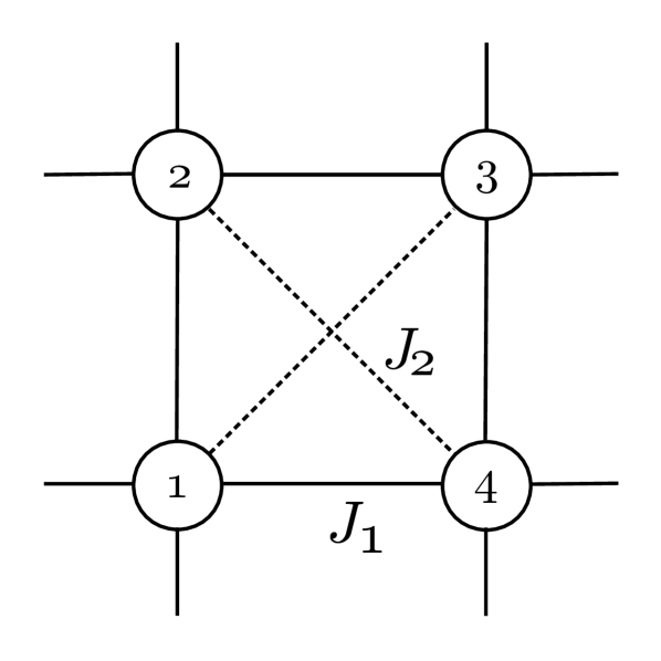
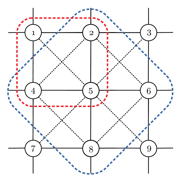
Where refers to the mean magnetization along the preferred direction of the system, of the site i, inside a given plaquette, following the convention showed in Fig.1.
While translational order parameters are enough to determine the presence of stripes, they are not suited to detect the breaking of the rotational symmetry of the lattice. They take the same values in a paramagnetic and a nematic phase, yet the nematic phase shows a structure of the correlations similar to that of the stripes. This is natural if we think about this phase as an intermediate one in between the completely symmetric paramagnetic phase and the ordered stripes phase. Therefore, to characterize the nematic behavior we introduced an orientational order parameter defined as
| (4) |
where represents the correlation between sites and in the plaquette. All the order parameters are defined in a way that .
III Mean Field Approximations and Quantum Cluster Variational Method
In order to compute the order parameters relevant for the - model it is fundamental to obtain a good approximation of at least local magnetizations and correlations of neighboring spins. These quantities can be found from a knowledge of the local density matrices describing the joint statistics of these spins.
With a cluster expansion the free energy is approximated as a sum of contributions of selected regions or groups of variables. Each term of the sum depends on the local density matrix of the corresponding variables (spins). These regions are typically chosen to balance the accuracy and the computational cost of the calculations. The resulting approximated expression is to be understood as variational in terms of the local densities. The quality of the final results depends directly on the choice of regions, their size in relation to the correlation length, and how much mean-field is put the treatment of effective interactions and correlation between regions.
Among the many cluster approximations appearing in the literature, the approach known as Cluster Variational Method or CVM is remarkable because of the systematic treatment of different levels of complexity Yedidia et al. (2005); Kikuchi (1951). In a natural way one can choose free energy expansions ranging from naive mean field, a Bethe approximation or more involved structures. A quantum extension of such ideas, QCVM, was developed in Morita (1994); Morita and Tanaka (1994); Tanaka et al. (1994) and more recently expanded in Domínguez and Mulet (2018). In particular we are interested in a construction called Kikuchi approximation. The Kikuchi free energy consists of a sum of local free energies of all the square unit cells (), the interacting pairs () formed by the overlap of neighbor cells111The diagonal interactions do not belong to any overlap region and therefore, according to the CVM, they do not appear explicitly as independent terms in the approximated free energy. and all the contributions from single spins ():
| (5) |
The local free energy terms are defined the usual way
| (6) |
where may label a plaquette, link or spin region. The numbers are weight factors that compensate the effect of overlap between regions. Due to overlaps, the contribution of some variables might be under or over represented if the weight factors were absent. For the case of interest here, .
The minimization of the functional should be done under certain constraints. In addition to the usual normalization conditions, , the consistency between different regions must be enforced explicitly. For all plaquettes and any of its forming links one could demand that the partial trace over spins and equals the link density :
| (7) |
Moreover, every link distribution could be forced to marginalize onto the corresponding spin densities and :
| (8) |
However, numerical resultsDomínguez and Mulet (2018) have shown that the above constraint scheme is too restrictive. It turns out that the minimization gives much more accurate results if consistency is enforced only in the direction of the spin-spin interactions. In this model, where interactions exist only in the OX direction, it amounts to relaxing (7) to the set of equations:
| (9) |
| (10) |
We are now in position to write a Lagrange function that includes the conditions (9) and (10) by means of suitable Lagrange multipliers , :
| (11) | |||||
| normalization conditions |
To conform to (9) and (10), it suffices to introduce the parametrization222Notice that and are actually operators on the Hilbert space of the pairs and the single spins , respectively.:
| (12) | |||||
| (13) |
It is enough to make all real to guarantee that and are Hermitian, and consequently, that is real. Moreover, this parametrization ensures that the operators that satisfy the stationary condition are all positive, which is the fundamental property of density matrices (in addition to an unit trace, of course).
We will say that the value of the Lagrange function is stationary with respect to a change in the density if the linear part of the expansion of , in powers of , is zero. The operator is arbitrary but should be Hermitian, traceless and small enough to keep as a valid density operator, The Lagrange function will be stationary with respect to the set of all densities , by definition, if it is stationary in each one of them. The stationarity condition can be summarized in the following formula:
| (14) |
As an example, let us work out the form of the density matrix of an arbitrary spin at the stationary point. The part of that depends on a given is
| (15) | |||||
In (15) the only term that is somewhat involved to expand to first order in , when evaluating , is the one with the logarithm. The trick is to use perturbation theory to write the eigenvalues of using the eigenvalues and eigenvectors of :
| (16) | |||||
| (17) |
The trace with the logarithm is therefore written as
| (18) | |||||
In (18) we used that has a null trace. From the results above it is not hard to deduce the linear expansion of :
| (19) |
The stationarity condition applied to (19) implies the following relation
| (20) |
Now we use that is an arbitrary traceless Hermitian operator to state that the part in parenthesis in (20) is at most a constant times the identity, and therefore, must have the form:
| (21) |
with . The condition determines the value of . The form of (21) resembles a Boltzmann distribution where an effective interaction given by the Lagrange multipliers is added to the original local Hamiltonian.
The same procedure that leads to (21) can be used to find expressions for the rest of the density operators, that is, for pair and plaquette densities. The general structure will be the same: a Boltzmann distribution where the local Hamiltonian is modified by a number of effective interactions. These appear due to the consistency relations between regions and via the corresponding Lagrange multipliers. We skip these derivations and only write the final expressions for the Kikuchi approximation:
| (22) |
In (22) we used a linear transformation to write and as a function of new parameters and , respectively. These changed variables will of course inherit the structure of the originals, see (12) and (13):
| (23) |
The form of (12), (13) and (23) suggests that the Lagrange multiplier can be interpreted as effective local fields and a contribution to the interaction constants between spins when their explicit form is put into the equations (22). The plaquette-to-pair is composed of a terms that adds to the part of the original local Hamiltonian, and two effective fields acting on the spins of the pair . On the other hand, the pair-to-spin is formed by an effective field on , for every spin that belongs to . The role of these extra fields is to guarantee the consistency between the distributions, according to the restrictions imposed to the variational function.
The nature of the constraints directly implies that no effective fields (or modification to interaction constants) act in the transverse (OZ) direction. The reason being that no consistency is demanded on this axis. As a consequence, moments and correlations in the OZ direction may differ if computed from different local densities. Since all the observables we study here are in OX, where consistency holds, this discrepancy is not a serious complication.
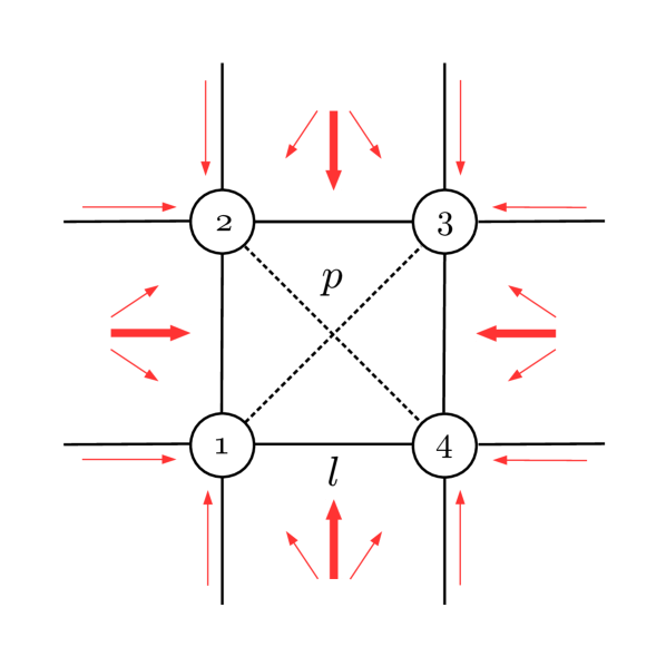
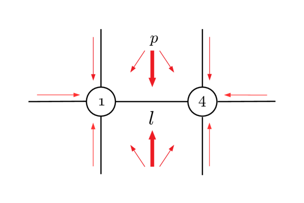
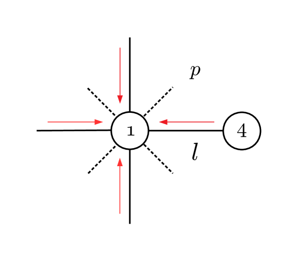
A graphical representation of the effective fields entering the formula (22) for the plaquette density operator is shown in Figure (2). Effective fields are drawn as arrows, placed according to the regions they are related to. For example, the arrows standing parallel to the edges of the lattice (NN interactions) correspond to terms. The arrows (triplet) pointing from the center of a square to a border pair picture the operators. In the same way, Figures (3) and (4) provide the representation for distributions and .
The final step to determine the local distributions is to find the value of the effective parameters. Their value is fixed by the solution of the set of equations imposed by the consistency relations (9) and (10). The numerical algorithm used to solve these coupled equations is very similar to the classical generalization of the well known Belief Propagation and is described in detail in Domínguez and Mulet (2018).
The basic scheme is the following. All effective fields are initialized in an arbitrary way (randomly, uniform, following a certain pattern, etc). Then, a series of update steps are performed until convergence is achieved333In certain cases the algorithm fails to converge. This will be discussed afterwards together with the numerical results.. We understand convergence as the situation where the values of the effective fields are such that all the consistency relations are satisfied simultaneously.
Let us describe a typical iteration for the field [upper triplet in Figure (3)]. First, compute using the current value of the fields depicted in Figure (2). Then, from determine the correlation and the magnetizations , . The crucial part is to use the consistency condition between and . We should find a value for the three components of (this parameter enters the formula for and not ) such that the observables computed from the pair distribution match the plaquette predictions:
| (24) | ||||
| (25) | ||||
| (26) |
The three equations above suffice to find the three parameters . The newly found value of is then updated in the lattice444Actually, what is usually stored is a weighted sum of the new and the old values. This procedure introduces a kind of damping that might help convergence..
Updating a pair-to-spin field, for example follows a similar recipe. First compute using the fields of Figure (3). Then compute the spin 1 magnetization using . Finally, find a value such that the same magnetization computed with matches the value computed with the pair distribution.
The algorithm described here assumes that we are using a given realization of the model, that is, that we are computing all the effective fields for every region defined in a square latice. The procedure is general and can handle situations where the external fields applied may not be homogeneous or the interactions change across the lattice. However, since the model in question is translationally invariant, it is reasonable to expect a simplification of the calculations; one would hope this structure is reflected in a translational symmetry of the effective fields. This is indeed the case. If the same values repeat all over the lattice, it is not necessary to solve equations but only a reduced set. The fields outside a certain region of the lattice can be taken as the same computed inside that region. In this case the numerical procedure looks like a self-consistent iteration. The idea, though, is not that every site in the lattice is equivalent to the rest, that is a too restrictive assumption that would allow only homogeneous states. The correct procedure is to consider the smallest possible structures that, by repetition, can create the patterns observed experimentally. In practice, to generate a pattern of stripes, or an anti-ferromagnetic checkerboard design, it is enough to consider a square plaquette as the elementary region. For the model studied here we followed both approaches, a specific realization of the lattice solving equations, and the more practical reduced version obtained equivalent results. For generality we will present only simulations results for the former method. On one hand it makes clearer the strength of QCVM for more general situations, on the other, makes more transparent when the algorithm does not converge.
To close this section we would like to make a few comments about our choice of the QCVM as the inference method used to compute the local observables of the - model. Mean field cluster approximations frequently found in the literature Kellermann et al. (2019); Balcerzak et al. (2018); Bobák et al. (2018) are often based on some kind of variational argument on single site spin magnetizations. In many cases the effect is equivalent to factoring out the correlations as products of single site moments. A more consistent treatment is expected to take into account more structure into the relevant correlations among the system variables. That is precisely the formal advantage of QCVM: by means of the effective interactions the correlations have extra parameters that can be used for tuning. This can lead to more precision in the prediction of system properties. A quick test, for example, shows that the Cluster Mean Field of Kellermann et al. (2019) applied to a classical Ising model on a square lattice returns predictions for the para-ferro transition temperature, that is closer to the naive MF prediction than to the real value . Bethe-Pierls approximation or Kikuchi give much more accurate estimates (2.89 and 2.41 respectively).
Mean field treatments usually replace real interactions by the interaction with the mean value of certain variables. For example, terms like might be roughly approximated by or something similar, which looks like an effective field acting on . QCVM effective fields can be understood in a similar way. With this in mind, we would like to point to what might be a caveat in the choice of regions used in the Kikuchi approximation. Since the overlap of elementary plaquettes corresponds only to NN pairs, the effective fields will only appear for those interactions. Notice for example the scheme for the single site distribution in Figure (4), where no diagonal effective fields are present. It would be desirable to have a setup where consistency is also forced for diagonal distributions which would then appear as diagonal effective fields. We believe this could be achieved if the elementary plaquettes are defined with a rhombic shape as shown in Figure (5).
IV Results and Discussion
IV.1 Summary of the classical model
We start this section presenting the phase diagram of the classical version of the model derived using the Cluster Variational MethodDomínguez et al. (2019). On one hand, it may help to understand better the effects of quantum fluctuations, on the other it serves as a checking point to probe that the approximation reproduces the known phenomenology of the model.
In short, as is shown in Fig.6, depending of the Temperature and the ratio the model may be in one of three phases, ferromagnetic, stripes or paramagnetic Jin et al. (2012). The lines are guides to the eyes, and the symbols represent the predicted order of the transition, continuous (closed), discontinuous (open).

The ground state in the low regime is Ferromagnetic, and the systems behaves essentially as an Ising ferromagnet with a continuous phase transition between the ferromagnetic and the paramagnetic phases. When the critical temperature predicted by the approximation is around , which is close to the exact critical value . In this branch of the phase diagram we notice also a grey zone separating the ferromagnetic and the paramagnetic phases for . This is a zone of non-convergence of the algorithm associated with oscillations due to the existence of the two symmetric solutions of the ferromagnetic phase. This zone will appear also in the presence of quantum fluctuations and is discussed in more detail in the Appendix A.
On the other branch of the diagram the system shows a high temperature paramagnetic phase and a low temperature phase of stripes. However the line dividing the two phases is characterized by different kind of phase transitions. Notice that Jin et al, Jin et al. (2012) predicted that below the transition is discontinuous and above continuous. QCVM provides a similar picture, but with a larger . Nevertheless we need to remark that the definition of this critical point from numerical simulations is highly non trivial. For example, in Fig.7, we show the behavior of the free energy when the parameter changes. At (Fig.7a), we find a very clear hysteresis loop, a signature of a first order transition. On the other hand, for (Fig.7b), the free energy dependence is flat, and there is not evidence of any hysteresis. In the rest of the work the order of the phase transitions was determined both by considering the occurrence of hysteresis loops in the free energy and by making an interpolation of the Free Energy and studying the continuity of its derivative close to the transition as discussed in the previous sections. Results from both methods are equivalent.


In Fig.8 we show the behavior of the orientational and positional order parameters around the transition. For (Fig.8a), it can be observed a wide hysteresis loop when increases or decreases and a sharp jump in the order parameter, both indications of a discontinuous transition. On the other hand, (Fig.8b) for there is a continuous change in the order parameter when increases, suggesting a continuous transition. However, there is also a small hysteresis loop suggesting a possible discontinuous transition. We checked that it is rather a consequence of the stability of the paramagnetic solution for this approximation, which is always a valid solution of the fixed point equations.


The richness of this model becomes more evident in the presence of a longitudinal field. In this case (see Figure 9) for proper values of the temperature and the field a nematic phase separates the paramagnetic phase and the phase of stripes Guerrero et al. (2015); Domínguez et al. (2019).

Summarizing, in the absence of external fields the classical - model presents (depending on the value of ) two low temperature phases, ferromagnetic and stripes. Increasing the ferromagnet behaves essentially like an Ising ferromagnet with a continuous transition to a paramagnetic phase. The phase of stripes may have, depending on a continuous or discontinuous transition to the paramagnetic phase. On the other hand, and depending on the temperature, in the presence of a longitudinal field the stripe and nematic phases may be separated by a novel nematic phase.
IV.2 The role of quantum fluctuations
With the previous understanding of the classical model we now concentrate our attention in the main motivation of our work: the role of quantum fluctuations.

We first explore the behavior of the QCVM at low values of the temperature, , and in the absence of the longitudinal field, . In this regime, and in the absence of quantum fluctuations the system is either in a ferromagnetic or in a stripe phase (see Fig. 6). Once the transverse external field is turned on and increased the system eventually turns paramagnetic with both, the orientational and positional order falling to zero as is shown in Fig.10.
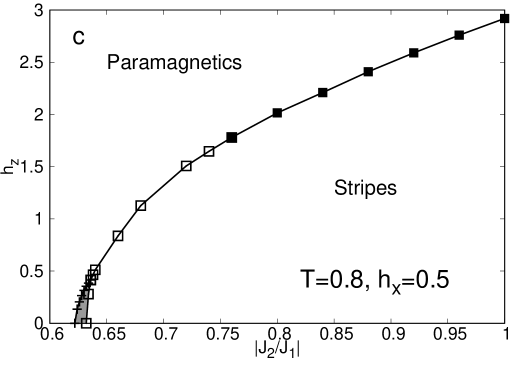
An extensive study of the parameters of the model at low temperatures allows the construction of the phase diagram (see Figure 11). Also in this case the ground state for is a ferromagnet, and the phase transition is continuous. Moreover, the predicted critical field at , corresponding to the quantum Ferromagnetic Ising Model is around Domínguez and Mulet (2018), which is close to the exact value Bikas K. Chakrabarti (1996). In the right branch of the diagram, the critical point, where the discontinuous transition between the phase of stripes and the paramagnetic phase becomes continuous is around , with . This value is also similar to the one reported by means of a Cluster Mean Field approach in Kellermann et al. (2019) (). On the other hand, QCVM for predicts a critical transverse field , much lower than the one reported in Kellermann et al. (2019), .
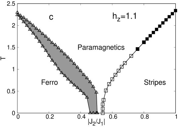
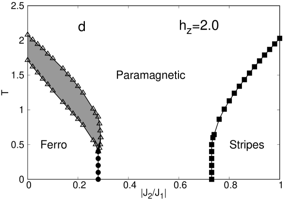
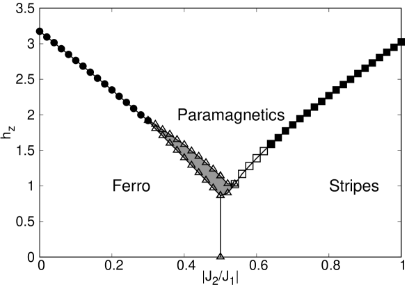
The effect of quantum fluctuations reshapes the classical phase diagram presented in Figure 6. This is shown in Fig. 12. At low values of , quantum fluctuations just extend the range of values of the ratio at which the paramagnetic to stripe transitions is continuous, i.e., in practice shifting to the left. On the other hand, when the transverse field is large enough (), quantum fluctuations induce a gap between the ferromagnetic and the phase of stripes that is ocupied by the paramagnetic phase. In this case, only when the frustration is very small or when it is very large the system exhibits actual order at low temperatures.

To summarize, we show in Fig.13 the vs phase diagrams for different values of the ratio . Three different scenarios are well characterized. For example, if , we find a full line of discontinuous phase transitions. In the other extreme, when , there is only continuous transitions, while at intermediate values of the frustration (for example, ), we can observe a line of mixing continuous and discontinuous phase transitions. In other words, in the presence of quantum fluctuations, the frustration favors the occurrence of continuous transitions.
IV.3 Quantum fluctuations in the presence of a longitudinal field
In this section we study the model in the presence of a longitudinal field, . As we already discussed, in the absence of the transverse field, the presence of a longitudinal field induces a nematic phase that separates the paramagnetic and the phase of stripes in a wide range of temperatures (see Figure 9). We will show that quantum fluctuations make this scenario more plausible with a nematic phase that may penetrate the phase of stripes.
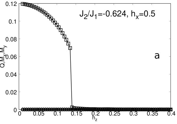
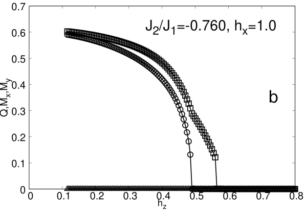
To have a glance on the effect of the longitudinal field in the picture discussed so far, in Fig.14 we show the behavior of the orientational and positional order parameters against the transverse field for different values of the ratio and the field . It can be observed that depending on the values of and the system may well have only orientational order but lack of translation order () if is small enough (panel a), or alternatively (panel b), a phase of stripes for low values of in which both and are different from zero. The first is a signature of the nematic phase and a transition from a nematic to a paramagnetic phase due to quantum fluctuations. In the second case, a scenario like that in panel b may take place in which, increasing , first the magnetizations structure homogenizes, continuously driving the system into a nematic phase, and only later when , the orientational order parameter (), drops abruptly to zero.
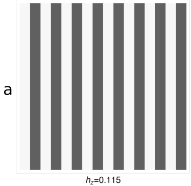
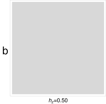
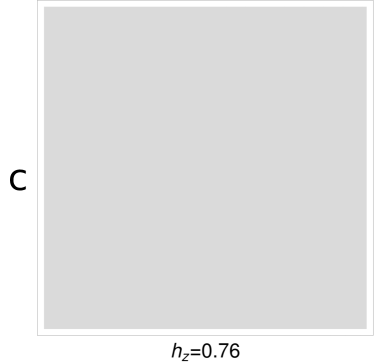
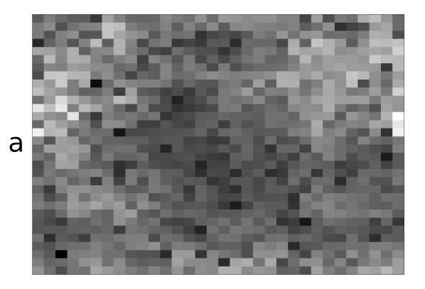
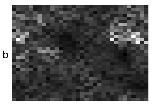
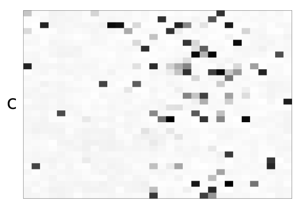
A clearer picture of the situation appears studying the evolution of the correlation and magnetization structure in the lattice as in Fig.15 for different values of . In this picture the correlation structure is represented using solid (dashed) lines to represent positive (negative) correlations, with a width proportional to their modulus. In Fig.15a, we can observe a clear structure of stripes, but with the subtle feature that the global magnetization is not zero, as the sites with positive magnetizations (white stripes) have a larger module than those pointing in the opposite direction. This is a consequence of the application of a field in a direction that breaks the symmetry between the two orientations, positive and negative. Another remarkable feature is that the correlation between different stripes (dashed lines) are lower compared to that between elements of the same stripes (solid lines). As the transverse field increases, we approach the nematic phase, represented in Fig.15b. There we can observe an homogeneous magnetization, yet a clear remainder of the stripes is observed in the correlation structure. Even when both correlations are positives we can clearly see that the line joining sites of the same column are represented with wider lines than those between different stripes. Lastly, in Fig.15c, we observed the paramagnetic phase corresponding to , slightly beyond the transition point. Clearly, this paramagnetic phase is “polarized”(i.e: no zero net magnetization), due to the external magnetic field.


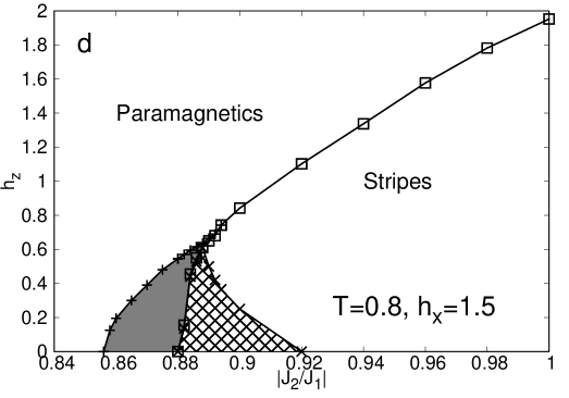
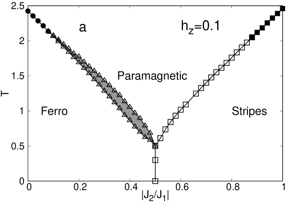
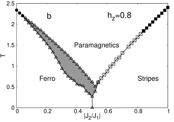
The behaviour of the order parameters can be condensed in the phase diagrams presented in Figure 16 for different values of and . At low temperatures (Figure 16a,b) it can be observed that the longitudinal field () changes the character of the transition. For example, in Figure 16(a), corresponding to a low longitudinal field, we have a line of continuous and discontinuous transitions, with a critical point separating the two behaviors while in panel b, (larger longitudinal field) all the transition line is discontinuous. So, we are tempted to associate the application of a larger longitudinal field with an increase in the discontinuous character of the phase transition. On the other hand, at higher temperatures, (Fig.16c and Fig.16d), a nematic phase shows up penetrating the phase of stripes. As can be easily observed, this region broadens as we increase the value of the longitudinal field. On the other side, we can check that as frustration increase (), the longitudinal field required for the occurrence of the nematic phase is larger. Notice also that in panel d, we have a non convergence region due to numerical issues in the implementation, which is quite demanding in this region of the phase diagram.

These results suggest that the nematic phase does not appear in a low temperature scenario in agreement with results previously observed Domínguez et al. (2019) in the classical model for . To further support this, in Fig.17, we show the behavior of the order parameters for . There we can clearly check that the nematic phase arises only after a certain threshold in .
Another feature of these phase diagrams that is worth mentioning is the effect of in the continuity of the phase transitions. The region in which first order transition occurs widens as increases. This effect goes in the opposite direction to the one we observe under the application of a transverse field. In Fig. 18, we show the phase diagram for , . The transition line is first order at low values of the transverse field, and large longitudinal one. In the other extreme case, a continuous transition occurs. The critical point is located around , .

V Conclusions
In this work we studied the quantum - model with nearest neighbor ferromagnetic interactions () and next nearest neighbour anti-ferromagnetic interactions () in the presence of a transverse field using the Quantum Cluster Variational Method. We study the model in an extensive lattice without particular assumptions about the symmetry of the problem. Our results show that quantum fluctuations change the order of the transition, the larger the quantum effects the wider is the range of parameters for which the transition is continuous. Moreover, quantum fluctuations may induce a gap between the ferromagnetic phase and the phase of stripes and in the presence of longitudinal fields also a pronounced nematic phase that penetrates the phase of stripes. This nematic phase is characterized by the presence of orientational order and the lack of translational order.
Appendix: On the convergence of QCVM near the continuous-discontinuous transition
Wide non convergence regions are observed in some of the - phases diagrams in Fig.12, as well as in the - in Fig.11. These non-convergence regions are characterized by an oscillatory behavior of the system, which can be observed in Fig.19. In this figure we show both the behavior of a single site’s magnetization as well as the global magnetization in a 32 x 32 lattice. Both values oscillate coherently, which is the signature of a global coordination rather than the result of single site isolated variations. An important thing to notice is that there is a decrease in the amplitude of the oscillations as we move from the ferromagnetic region to the paramagnetic one.

Fig.20 displays the magnetization structure of a 32 x 32 lattice inside the non convergence region. According to what was previously shown in Fig.19, there is a large coordination between most of the sites of the lattice.
For much larger regions, say , both the global and local magnetization keep oscillating coherently, yet the global magnetization does it with a shorter amplitude (Fig.21).

This effect can be linked to the formation of clusters. In order to further motivate this statement we first show in Fig.22 the oscillations of the magnetization of a site chosen randomly and some of its neighbors. We can observe what can be described as a local coordination.

Finally, in Fig.23, we show the 64 x 64 lattice structure for two different time steps. It can be directly observed in the two cases, the formation of clusters of sites pointing in the same direction, which visually show what we supposed was the reason for the apparent contradiction in the oscillation of the local and global magnetization.
References
- Sachdev (1999) S. Sachdev, Quantum Phase Transitions (Cambridge University Press, Cambridge, UK, 1999).
- Fradkin (2013) E. Fradkin, Field Theories of Condensed Matter Physics (Cambridge University Press, Cambridge, UK, 2013).
- Shankar (2017) R. Shankar, Quantum Field Theory and Condensed Matter Physics (Cambridge University Press, Cambridge, UK, 2017).
- Bobák et al. (2018) A. Bobák, E. Jurcisinová, M. Jurcisin, and M. Zukovic, Physical Review E 98, 022124 (2018).
- Jin et al. (2013) S. Jin, A. Sen, W. Guo, and A. W. Sandvik, Physical Review B 87, 144406 (2013).
- Ren et al. (2014) Y.-Z. Ren, N.-H. Tong, and X.-C. Xie, Journal of Physics: Condensed Matter 26, 115601 (2014).
- Yamamoto (2008) D. Yamamoto, arxiv:0812.4139 (2008).
- F.M. et al. (2016) Z. F.M., S. M., and M. J., arxiv:1604.03486 (2016).
- Singhania and Kumar (2018) A. Singhania and S. Kumar, Physical Review B 98, 104429 (2018).
- Domínguez and Mulet (2018) E. Domínguez and R. Mulet, Physical Review B 97, 064202 (2018).
- Mézard and Montanari (2009) M. Mézard and A. Montanari, Information, Physics and Computation (Oxford University Press, Cambridge, 2009).
- Morita (1994) T. Morita, Progress of Theoretical Physics 92, 1081 (1994).
- Morita and Tanaka (1994) T. Morita and T. Tanaka, Progress of Theoretical Physics 92, 1081 (1994).
- Tanaka et al. (1994) T. Tanaka, K. Hirose, and K. Kurati, Progress of Theoretical Physics Supplement 115, 41 (1994).
- Rizzo et al. (2010) T. Rizzo, A. Lage-Castellanos, R. Mulet, and F. Ricci-Tersenghi, J. Stat. Phys. 139, 375 (2010).
- Domínguez et al. (2011) E. Domínguez, A. Lage, R. Mulet, F. Ricci-Tersenghi, and T. Rizzo, J. Stat. Mech. , P12007 (2011).
- Lage-Castellanos et al. (2013) A. Lage-Castellanos, R. Mulet, F. Ricci-Tersenghi, and T. Rizzo, Journal of Physics A: Mathematical and Theoretical 46, 135001 (2013).
- Evans and Stephens (2008) Z. W. E. Evans and A. M. Stephens, Physical Review A 78, 062317 (2008).
- Leifer and Poulin (2008) M. Leifer and D. Poulin, Annals of Physics 323, 1899 (2008).
- Poulin and Bilgin (2008) D. Poulin and E. Bilgin, Physical Review A 77, 052318 (2008).
- Bilgin and Poulin (2009) E. Bilgin and D. Poulin, arxiv: 0910.2299 (2009).
- Poulin and Hastings (2011) D. Poulin and M. B. Hastings, Physical Review Letters 106, 080403 (2011).
- Jouneghani et al. (2014) F. G. Jouneghani, M. Babazadeh, D. Salami, and H. Movla, arxiv:1409.2048.v1 (2014).
- Biazzo and Ramezanpour (2013) I. Biazzo and A. Ramezanpour, Journal of Statistical Mechanics: Theory and Experiment 2013, P04011 (2013).
- Biazzo and Ramezanpour (2014) I. Biazzo and A. Ramezanpour, Physical Review E 89, 062137 (2014).
- De’ Bell et al. (2000) K. De’ Bell, A. B. MacIsaac, and J. P. Whitehead, Review of Modern Physics 72, 225 (2000).
- Díaz-Méndez and Mulet (2010) R. Díaz-Méndez and R. Mulet, Physical Review B 81, 184420 (2010).
- Fey and Schmidt (2016) S. Fey and K. Schmidt, Physical Review B 94, 075156 (2016).
- Fey et al. (2019) S. Fey, S. C. Kapfer, and K. P. Schmidt, Physical Review Letters 122, 017203 (2019).
- Mendoza-Coto et al. (2015) A. Mendoza-Coto, D. A. Stariolo, and L. Nicolao, Physical Review Letters 114, 116101 (2015).
- Mendoza-Coto et al. (2017) A. Mendoza-Coto, D. G. Barci, and D. A. Stariolo, Physical Review B 95, 144209 (2017).
- Mendoza-Coto et al. (2020) A. Mendoza-Coto, D. E. B. de Oliveira, L. Nicolao, and R. Díaz-Méndez, Physical Review B 101, 174438 (2020).
- Cannas et al. (2006) S. A. Cannas, M. F. Michelon, D. A. Stariolo, and F. A. Tamarit, Physical Review B 73, 184425 (2006).
- Nandkishore and Sondhi (2010) R. M. Nandkishore and S. Sondhi, Physical Review X 7, 041021 (2010).
- Oganesyan and Huse (2007) V. Oganesyan and D. A. Huse, Physical Review B 75, 155111 (2007).
- Bruun and Taylor (2008) G. Bruun and E. Taylor, Physical Review Letters 101, 245301 (2008).
- Parish and Marchetti (2012) M. Parish and F. Marchetti, Physical Review Letters 108, 145304 (2012).
- Morán-López et al. (1993) J. L. Morán-López, F. Aguilera-Granja, and J. M. Sanchez, Physical Review B 48, 3519 (1993).
- Moran-Lopez et al. (1994) J. L. Moran-Lopez, F. Aguilera-Granja, and J. M. Sanchez, Journal of Physics: Condensed Matter 6, 9759 (1994).
- Guerrero et al. (2015) A. I. Guerrero, D. A. Stariolo, and N. G. Almarza, Physical Review E 91, 052123 (2015).
- Domínguez et al. (2019) E. Domínguez, A. Lage-Castellanos, C. Lopetegui, and R. Mulet, Revista Cubana de Física 36, 20 (2019).
- dos Anjos et al. (2008) R. A. dos Anjos, J. R. Viana, and J. R. de Sousa, Physics Letters A 372, 1180 (2008).
- Kalz et al. (2009) A. Kalz, A. Honecker, S. Fuchs, and T. Pruschke, Journal of Physics: Conference Series 145, 012051 (2009).
- Kalz et al. (2011) A. Kalz, A. Honecker, and M. Moliner, Physical Review B 84, 174407 (2011).
- Jin et al. (2012) S. Jin, A. Sen, and A. W. Sandvik, Physical Review Letters 108, 045702 (2012).
- Kohama et al. (2019) Y. Kohama, H. Ishikawa, A. Matsuo, K. Kindo, N. Shannon, and Z. Hiroi, Proceedings of the National Academy of Sciences 116, 10686 (2019).
- Shannon et al. (2004) N. Shannon, B. Schmidt, K. Penc, and P. Thalmeier, The European Physical Journal B - Condensed Matter and Complex Systems 38, 599 (2004).
- Mezzacapo (2012) F. Mezzacapo, Phys. Rev. B 86, 045115 (2012).
- Jiang et al. (2012) H.-C. Jiang, H. Yao, and L. Balents, Physical Review B 86, 024424 (2012).
- Dagotto and Moreo (1989) E. Dagotto and A. Moreo, Physical Review Letters 63, 2148 (1989).
- Shindou et al. (2013) R. Shindou, S. Yunoki, and T. Momoi, Physical Review B 87, 054429 (2013).
- Cysne and Neto (2015) T. P. Cysne and M. B. S. Neto, EPL (Europhysics Letters) 112, 47002 (2015).
- Carretta et al. (2002) P. Carretta, N. Papinutto, C. B. Azzoni, M. C. Mozzati, E. Pavarini, S. Gonthier, and P. Millet, Physical Review B 66, 094420 (2002).
- Melzi et al. (2001) R. Melzi, S. Aldrovandi, F. Tedoldi, P. Carretta, P. Millet, and F. Mila, Physical Review B 64, 024409 (2001).
- Nath et al. (2008) R. Nath, A. A. Tsirlin, H. Rosner, and C. Geibel, Physical Review B 78, 064422 (2008).
- Orlova et al. (2017) A. Orlova, E. L. Green, J. M. Law, D. I. Gorbunov, G. Chanda, S. Krämer, M. Horvatić, R. K. Kremer, J. Wosnitza, and G. L. J. A. Rikken, Physical Review Letters 118, 247201 (2017).
- Yedidia et al. (2005) J. Yedidia, W. T. Freeman, and Y. Weiss, IT-IEEE 51, 2282 (2005).
- Kikuchi (1951) R. Kikuchi, Phys. Rev. 81, 988 (1951).
- Kellermann et al. (2019) N. Kellermann, M. Schmidt, and F. M. Zimmer, Physical Review E 99, 012134 (2019).
- Balcerzak et al. (2018) T. Balcerzak, K. Szałowski, A. Bobák, and M. Žukovič, Phys. Rev. E 98, 022123 (2018).
- Bikas K. Chakrabarti (1996) P. S. a. Bikas K. Chakrabarti, Amit Dutta, Quantum Ising Phases and Transitions in Transverse Ising Models, Lecture Notes in Physics Monographs 41 (Springer Berlin Heidelberg, 1996).