The Rate Loss of Single-Letter Characterization:
The “Dirty” Multiple Access Channel
Abstract
For general memoryless systems, the typical information theoretic solution - when exists - has a “single-letter” form. This reflects the fact that optimum performance can be approached by a random code (or a random binning scheme), generated using independent and identically distributed copies of some single-letter distribution. Is that the form of the solution of any (information theoretic) problem? In fact, some counter examples are known. The most famous is the “two help one” problem: Korner and Marton showed that if we want to decode the modulo-two sum of two binary sources from their independent encodings, then linear coding is better than random coding. In this paper we provide another counter example, the “doubly-dirty” multiple access channel (MAC). Like the Korner-Marton problem, this is a multi-terminal scenario where side information is distributed among several terminals; each transmitter knows part of the channel interference but the receiver is not aware of any part of it. We give an explicit solution for the capacity region of a binary version of the doubly-dirty MAC, demonstrate how the capacity region can be approached using a linear coding scheme, and prove that the “best known single-letter region” is strictly contained in it. We also state a conjecture regarding a similar rate loss of single letter characterization in the Gaussian case.
Index Terms:
Multi-user information theory, random binning, linear lattice binning, dirty paper coding, lattice strategies, Korner-Marton problem.I Introduction
Consider the two-user / double-state memoryless multiple access channel (MAC) with transition and state probability distributions
| (1) |
respectively, where the states and are known non-causally to user and user , respectively. A special case of (1) is the additive channel shown in Fig. 1. In this channel, called the doubly-dirty MAC (after Costa’s “writing on dirty paper” [1]), the total channel noise consists of three independent components: and , the interference signals, that are known to user and user , respectively, and , the unknown noise, which is known to neither. The channel inputs and may be subject to some average cost constraint.
Neither the capacity region of (1) nor that of the special case of Fig. 1 are known. In this paper we consider a particular binary version of the doubly-dirty MAC of Fig. 1, where all variables are in , i.e., , and the unknown noise . The channel output of the binary doubly-dirty MAC is given by
| (2) |
where denotes the addition (xor), and are and independent. Each of the codewords is a function of the message and the interference vector , and must satisfy the input constraint, , , where and is the Hamming weight. The coding rates and of the two users are given as usual by , where is the set of messages of user , and is the length of the codeword.
The double state MAC (1) generalizes the point to point channel with side information (SI) at the transmitter considered by Gel’fand and Pinsker [2]. They prove their direct coding theorem using the framework of random binning, which is widely used in the analysis of multi-terminal source and channel coding problems [3]. They obtain a general capacity expression which involves an auxiliary random variable :
| (3) |
where the maximization is over all the joint distributions of the form .
The channel in (1) with only one informed encoder (i.e., where ) was considered recently by Somekh-Baruch et al. [4] and Kotagiri and Laneman [5]. The common message () capacity of this channel is known [4], and it involves using random binning by the informed user. For the binary “one dirty user” case (i.e., (2) with ), we show that Somekh-Baruch’s common-message capacity becomes (see Appendix A)
| (4) |
where is the binary entropy function. Clearly, the doubly-dirty individual-message case is harder. Thus, it follows from (4) that the rate-sum in the setting of Fig. 1 is upper bounded by
| (5) |
In Theorem 1 we show that this upper bound is in fact tight.
One approach to find achievable rates for the doubly-dirty MAC, is to extend the Gel’fand and Pinsker solution [2] to the two-user / double-state case. As shown by Jafar [6], this extension leads to the following pentagonal inner bound for the capacity region of (1):
| (6) | ||||
for some . In fact, by a standard time-sharing argument [3], the closure of the convex hull of the set of all rate pairs satisfying (7),
| (7) |
is also achievable111 As in the Gel’fand and Pinsker solution, for a finite alphabet system it is enough to optimize over auxiliary variables and whose alphabet size is bounded in terms of the size of the input and state alphabets. . To the best of our knowledge, the set is the best currently known single-letter characterization for the rate region of the MAC with side information at the transmitters (1), and in particular, for the doubly-dirty MAC (2)222For the case where the users have also a common message to be transmitted jointly by both encoders, (7) can be improved by adding another auxiliary random variable which plays the role of the common auxiliary r.v. in Marton’s inner bound for the non-degraded broadcast channel [7]. In this case, the joint distribution of is given by , i.e, and are conditionally independent given .. The achievability of (7) can be proved, as usual, by an i.i.d random binning scheme [6].
A different method to cancel known interference is by “linear strategies”, i.e, binning based on the cosets of a linear code [8, 9, 10]. In the sequel, we show that the outer bound (5) can indeed be achieved by a linear coding scheme. Hence, the set of rate pairs satisfying (5) is the capacity region of the binary doubly-dirty MAC. In contrast, we show that the single-letter region (7) is strictly contained in this capacity region. Hence, a random binning scheme based on this extension of the Gel’fand-Pinsker solution [2] is not optimal for this problem.
A similar observation has been made by Korner-Marton [11] for the “two help one” source coding problem. For a specific binary version known as the “modulo-two sum” problem, they showed that the minimum possible rate sum is achieved by a linear coding scheme, while the best known single-letter expression for this problem is strictly higher. See the discussion in [11, Section IV] and in the end of Section III.
Although the “single-letter characterization” is a fundamental concept in information theory, it has not been generally defined [12, p.35]. Csiszar and Korner [13, p.259] suggested to define it through the notion of computability, i.e., a problem has a single-letter solution if there exists an algorithm which can decide if a point belongs to an -neighborhood of the achievable rate region with polynomial complexity in . Since we are not aware of any other computable solution to our problem, we shall refer to (7) as the “best known single-letter characterization”.
An extension of these observations to continuous channels would be of interest. Costa [1] considered the single-user case of the dirty channel problem , where the interference and the noise are assumed to be i.i.d. Gaussian with variances and , respectively, and the input is subject to a power constraint . He showed that in this case, the transmitter side-information capacity (3) coincides with the zero-interference capacity , where . Selecting the auxiliary random variable in (3) such that
| (8) |
where and are independent, and taking , the formula (3) and its associated random binning scheme are capacity achieving. The continuous (Gaussian) version of the doubly-dirty MAC of Fig. 1 was considered in [10]. It was shown that by using a linear structure, i.e., lattice strategies [8], the full capacity region is achieved in the limit of high SNR and high lattice dimension. In contrast, it was shown that for no positive rate is achievable by using the natural generalization of Costa’s strategy (8) to the two user case, while a (scalar) modulo addition version of (8) looses bit in the sum capacity. We shall further elaborate on this issue in Section IV.
Similar observations regarding the advantage of modulo-lattice modulation with respect to a separation based solution were made by Nazer and Gastpar [14], in the context of computation over linear Gaussian networks, and also by Krithivasan and Pradhan [15] for multi-terminal rate distortion problems.
The paper is organized as follows. In Section II the capacity region for the binary doubly-dirty MAC (2) is derived, and linear coding is shown to be optimal. Section III develops a closed form expression for the best known single-letter characterization (7) for this channel, and demonstrates that it is strictly contained in the the true capacity region. In Section IV we consider the Gaussian doubly-dirty MAC, and state a conjecture regarding the capacity loss of single-letter characterization in this case.
II The Capacity Region of the Binary Doubly-Dirty MAC
The following theorem characterizes the capacity region of the binary doubly-dirty MAC of Fig. 1.
Theorem 1.
The capacity region of the binary doubly-dirty MAC (2) is the set of all rate pairs satisfying
| (9) |
Proof.
The converse part: As explained in the Introduction (5), one way to derive an upper bound for the rate-sum is through the general one-dirty-user capacity formula [4], which we derive explicitly for the binary case in Appendix A. Here we show directly the converse part, which is similar to the proof of the outer bound for the Gaussian case in [16, 10]. We assume that user and user intend to transmit a common message . An upper bound on the rate of this message clearly upper bounds the sum rate in the individual messages case. Thus,
| (10) | ||||
| (11) | ||||
| (12) | ||||
| (13) | ||||
| (14) | ||||
| (15) |
where (10) follows from Fano’s inequality where as the error probability goes to zero for ; (11) follows since is fully known given , and ; (12) follows from the chain rule for entropy, and due to and since , and are mutually independent; (13) follows since and ; (14) follows since is a function of , finally (15) follows since .
In the same way we can show that . The converse part follows since for we have that , thus .
The direct part is based on the scheme for the point-to-point binary dirty paper channel [9]. We define . In view of the converse part, it is sufficient to show achievability of the point , since the outer bound may be achieved by time sharing with the symmetric point . The corner point corresponds to the “helper problem”, i.e., user tries to help user to transmit at its highest rate. The encoders and decoder are described using a binary linear code with parity check matrix . Let be a syndrome of the code , where we note that each syndrome represents a different coset of the linear code . Let denote the “leader” of (or the minimum weight vector in) the coset associated with the syndrome [17, Chap. 6], hence . For , we define the -dimensional modulo operation over the code as
which is the leader of the coset to which the vector belongs.
-
•
Encoder of user : Let the transmitted message be a syndrome in , and let be its coset leader. In particular . Transmit the modulo of the code with respect to the difference between and , i.e.,
-
•
Encoder of user : (functions as a “helper” for user ). Transmit
-
•
Decoder:
1. Reconstruct by .
2. Reconstruct the transmitted coset of user by .
In fact, the transmitted coset can be reconstructed directly as , where the last equality follows since and are in the same coset.
It follows that the decoder correctly decodes the message coset , since
where the third equality follows since and are in the same coset. It is left to relate the coding rate to the input constraint . Form [18], there exists a binary linear code with covering radius that satisfies where as . The achievability of the point follows by using , thus , while and , hence
This completes the proof of the direct part of the theorem. ∎
As stated above, the achievability for the capacity region follows by time sharing the corner points and where . It is also interesting to see how to achieve the rate sum for an arbitrary rate pair without time sharing. For that, let the message of user be and the message of user be where . We define the following syndromes in
Clearly, given the syndrome the syndromes and are fully known and the messages and as well. Let be the coset leader of for . In this case the transmission scheme is as follow:
-
•
Encoder of user : transmit .
-
•
Encoder of user : transmit .
-
•
Decoder: reconstruct .
Therefore, we have that
The sum capacity is achieved since where as which satisfies the input constraints.
III A Single-Letter Characterization for the Capacity Region
In this section we characterize the best known single-letter region (7) for the binary doubly-dirty MAC (2), and show that it is strictly contained in the capacity region (9). For simplicity, we shall assume identical input constraints, i.e., .
Definition 1.
In the following theorem we give a closed form expression for .
Theorem 2.
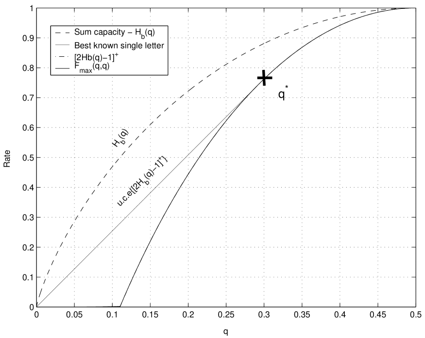
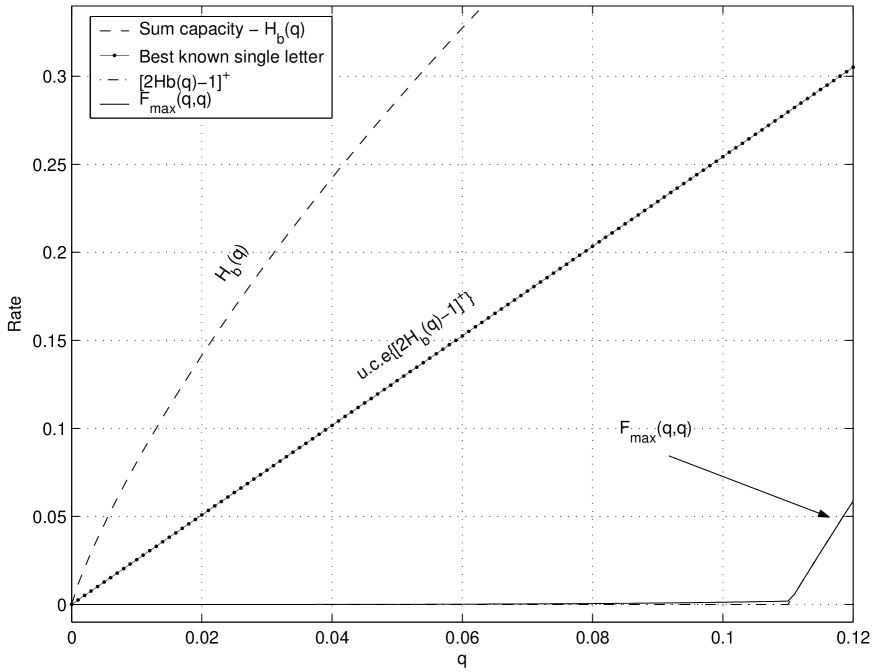
The best known single-letter rate region for the binary doubly-dirty MAC (2) is a triangular region given by
| (16) |
where is the upper convex envelope with respect to , and .
Fig. 2 shows the sum capacity of the binary doubly-dirty MAC (9) versus the best known single-letter rate sum (16) for equal input constraints. The latter is strictly contained in the capacity region which is achieved by a linear code. The quantity is not a convex - function with respect to . The upper convex envelope of is achieved by time-sharing between the points and , therefore it is given by
| (19) |
where .
Proof.
The direct part is shown by choosing in (6) and , where and are independent. From (6) the achievable rate sum is given by
| (20) | |||
| (21) | |||
| (22) | |||
| (23) |
where (20) follows since ; (21) follows from the chain rule for entropy; (22) follows since is fully known given thus ; (23) follows since and since are independent with thus .
The converse part of the proof is given in Appendix B. ∎
We see that the binary doubly-dirty MAC is a memoryless channel coding problem, where the capacity region is achievable by a linear code, while the best known single-letter rate region is strictly contained in the capacity region. This may be explained by the fact that each user has only partial side information, and distributed random binning is unable to capture the linear structure of the channel.
In order to understand the limitation of random binning versus a linear code, we consider these two schemes for high enough , that is . The random binning scheme uses where and are independent, therefore where for . Each transmitter maps the message (bin) into a codeword which is with high probability at a Hamming distance of from . Therefore, given the vectors , the available input space is approximately . Given the received vector , the residual ambiguity is given by , since and . As a result, the achievable rate sum is given by
The linear coding scheme shown in Theorem 1 has the same input space size as the random binning scheme, i.e., , since each user has cosets. However, given the received vector there are possible pairs of cosets, i.e., the residual ambiguity is only . Therefore, the linear code achieves rate sum of . The advantage of the linear coding scheme results from the “ordered structure” of the linear code, which decreases the residual ambiguity from bit in random coding to .
The following example illustrates the above arguments for the case that user is a “helper” for user , i.e, , and user transmits at his highest rate for each technique (random binning or linear coding). Table I summarizes the rates and codebooks sizes for each user for , that is bit.
| Random binning | Linear code | |
|---|---|---|
| Rate sum | bit | bit |
| Codewords per bin/coset | ||
| Helper (user ) - codebook size | ||
| User - codebook size | ||
| Number of possible codeword pairs |
Korner and Marton [11] observed a similar behavior for the “two help one” source coding problem shown in Fig. 3. In this problem, there are three binary sources , where , and the joint distribution of and is symmetric with . The goal is to encode the sources and separately such that can be reconstructed losslessly. Korner and Marton showed that the rate sum required is at least
| (24) |
and furthermore, this rate sum can be achieved by a linear code: each encoder transmits the syndrome of the observed source relative to a good linear binary code for a BSC with crossover probability .
In contrast, the “one help one” problem [19, 20] has a closed single-letter expression for the rate region, which corresponds to a random binning coding scheme. Korner and Marton [11] generalize the expression of [19, 20] to the “two help one” problem, and show that the minimal rate sum required using this expression is given by
| (25) |
The region (25) corresponds to Slepian-Wolf encoding of and , and it can also be derived from the Burger-Tung achievable region [21] for distributed coding for and with one reconstruction under the distortion measure . Clearly, the region (6) is strictly contained in the Korner-Marton region (24) (since for , where ). For further background on related source coding problems, see [15].
IV The Gaussian Doubly-Dirty MAC
In this section we introduce our conjecture regarding the rate loss of the best known single-letter characterization for the capacity region of the two-user Gaussian doubly-dirty MAC at high SNR. The Gaussian doubly-dirty MAC [10] is given by
| (26) |
where is independent of , and where user and user must satisfy the power constraints, and see Fig. 1. The interference signals and are known non-causally to the transmitters of user and user , respectively. We shall assume that and are independent Gaussian with variances going to infinity, i.e., where for . The signal to noise ratios for the two users are and .
The capacity region at high SNR, i.e., , is given by [10],
| (27) |
and it is achievable by a modulo lattice coding scheme of dimension going to infinity. In contrast, it was shown in [10] that at high SNR and strong independent Gaussian interferences, the natural generalization of Costa’s strategy (8) for the two users case, i.e., with auxiliary random variables and , is not able to achieve any positive rate. A better choice for and suggested in [10] is a modulo version of Costa’s strategy (8),
| (28) |
where , and where is independent of , for . In this case the rate loss with respect to (27) is .
The best known single-letter capacity region for the Gaussian doubly-dirty MAC (26) is defined as the set of all rate pairs satisfying (7), where and are restricted to the power constraints and . We believe that for high SNR and strong interference, the modulo- strategy (28) is an optimum choice for in (7) for the Gaussian doubly-dirty MAC. This implies the following conjecture about the rate loss of the best known single-letter characterization.
Conjecture 1.
Note that the right hand side of (29) is the well known “shaping loss” [22] (equivalent to a power loss).
A heuristic approach to attack the proof of this conjecture is to follow the steps of the proof of the converse part in the binary case (Theorem 2). First, in Lemma 6 we derive a simplified single-letter formula, , which is analogous to Lemma 1 in the binary case. The next step would be to optimize this expression. However, an optimal choice for the auxiliary random variables (provided in the binary case by Lemma 2 and Lemma 3) is unfortunately still missing for the Gaussian case. The expression in Lemma 6 is close in spirit to the point-to-point dirty tape capacity for high SNR and strong interference [8]. In [8] it is shown that optimizing the capacity is equivalent to minimum entropy-constrained scalar quantization in high resolution, which is achieved by a lattice quantizer. Clearly, if we could show a similar lemma for the two variable pairs in the maximization of Lemma 6, i.e., that it is achieved by a pair of lattice quantizers, then the conjecture would be an immediate consequence.
It should be noted that the above discussion is valid only for strong interferences and . For interference with finite power, it seems that cancelling the interference part of the time and staying silence the rest of the time (like in the time-sharing region in the binary case) may achieve better rates.
V Summary
A memoryless information theoretic problem is considered open as long as we are missing a general single-letter characterization for its information performance. This goes hand in hand with the optimality of the random coding approach for those problems which are currently solved. We examined this traditional view for the memoryless doubly-dirty MAC.
In the binary case, we showed that the best known single letter characterization is strictly contained in the region achievable by linear coding, and that the latter is in fact the full capacity region of the problem. In the Gaussian case, we conjectured that the best known single-letter characterization suffers an inherent rate loss (equal to the well known “shaping loss” ), and we provide a partial proof. This is in contrast to the asymptotic optimality (dimension ) of lattice strategies, as recently shown in [10].
The underlying reason for these performance gaps is that random binning is in general not optimal when side information is distributed among more than one terminal in the network. In the specific case of the doubly-dirty MAC (like in Korner-Marton’s modulo-two sum problem [11] and similar settings [14, 15]), the linear structure of the network allows to show that linear binning is not only better, but it is capacity achieving.
Appendix A A Closed Form Expression for the Capacity of the Binary MAC with One Dirty User
We consider the binary dirty MAC (2) with ,
| (30) |
where is known non-causally at the encoder of user with the input constraints for . We show that the common message () capacity of this channel is given by
| (31) |
To prove (31), consider the general expression for the common message capacity of the MAC with one informed user [4], given by
| (32) |
where the maximization is over al the joint distributions
The converse part of (31) follows since for any , the common message rate can be upper bounded by
| (33) | ||||
| (34) | ||||
| (35) | ||||
| (36) | ||||
| (37) |
where (33) follows since and ; (34) follows since ; (35) follows the definition ; (36) follows from the definition of the conditional entropy; (37) follows from the following definitions and for any . We also define , therefore the input constraint of user can be written as
| (38) |
Without loss of generality, we can only consider in (37) for any . Thus,
| (39) | ||||
| (40) | ||||
| (41) | ||||
| (42) |
where (39) follows from (37) and since , where ; (40) follows since is increasing in for and decreasing in for , thus the maximum is for ; (41) follows from Jensen’s inequality since is convex-; (42) follows from the input constraint for user (38). The converse part follows since the outer bound is valid for any and that satisfy the input constraints.
The direct part is shown by using where and are independent with , thus . Furthermore, which is independent of . In this case , hence . Using this choice for , the achievable common message rate is given by
| (43) | ||||
where (43) follows since , , and .
Appendix B Proof of the Converse Part of Theorem 2
The proof of the converse part follows from Lemma 1, Lemma 2 and Lemma 3, whereas Lemma 5 and Lemma 4 are technical results which assist in the derivation of Lemma 3.
Let us define the following functions:
| (44) |
where ; its -constrained maximization with respect to where and are independent, i.e.,
| (45) | ||||
and the upper convex envelope of with respect to
| (46) |
In the following lemma we give an outer bound for the single-letter region (7) of the binary doubly-dirty MAC in the spirit of [23, Lemma 3] and [8, Proposition 1].
Lemma 1.
Proof.
An outer bound on the best known single-letter region (7) is given by
| (48) | ||||
| (49) | ||||
| (50) | ||||
| (51) | ||||
| (52) | ||||
| (53) | ||||
| (54) | ||||
| (55) | ||||
| (56) |
where (50) follows since and ; (51) follows from the definition of the conditional entropy; (52) follows since ; (53) follows from the definition of the function (44), likewise (54) follows from the definition of the function (46), and from the definition
(55) follows from Jensen’s inequality since is a concave function; (56) follows from the input constraints where
| (57) |
The lemma now follows since the upper bound (56) for the rate sum is independent of and , hence it also bounds the single-letter region . ∎
A simplified expression for the function of (45) is shown in the following lemma.
Lemma 2.
Proof.
The function is defined in (44) and (45) where are binary random variables. Let us define the following probabilities:
for . We thus have
for . The maximization (45) can be written as
| (59) |
This maximization has two equivalent solutions and where , since any other can only increase the inner minimization in (59) which results in a lower . Therefore, without loss of generality we may assume that .
To prove the lemma we need to show that for any the inner minimization is achieved by
In other words, has the smallest possible probability for under the constraint that , implying that the transition from to is a “Z channel”. The inner minimization requires that will be minimized restricted to the constraint , therefore it is equivalent to the following minimization
For , the solution is and since in this case and the constraint is satisfied. For , in order to minimize , it is required that will be minimal and will be maximal such that the constraint is satisfied. Clearly, the best choice is for and , in this case the constraint is satisfies and . ∎
The next lemma gives an explicit upper bound for (45) for the case that . Let
| (60) |
and let
| (61) |
Since is differentiable, we can characterize by differentiating with respect to and equating to zero, thus we get that
This fourth order polynomial has two complex roots and two real roots, where one of its real roots is a local minimum and the other root is a local maximum. Specifically, this local maximum maximizes for the interval and it achieves which occurs at .
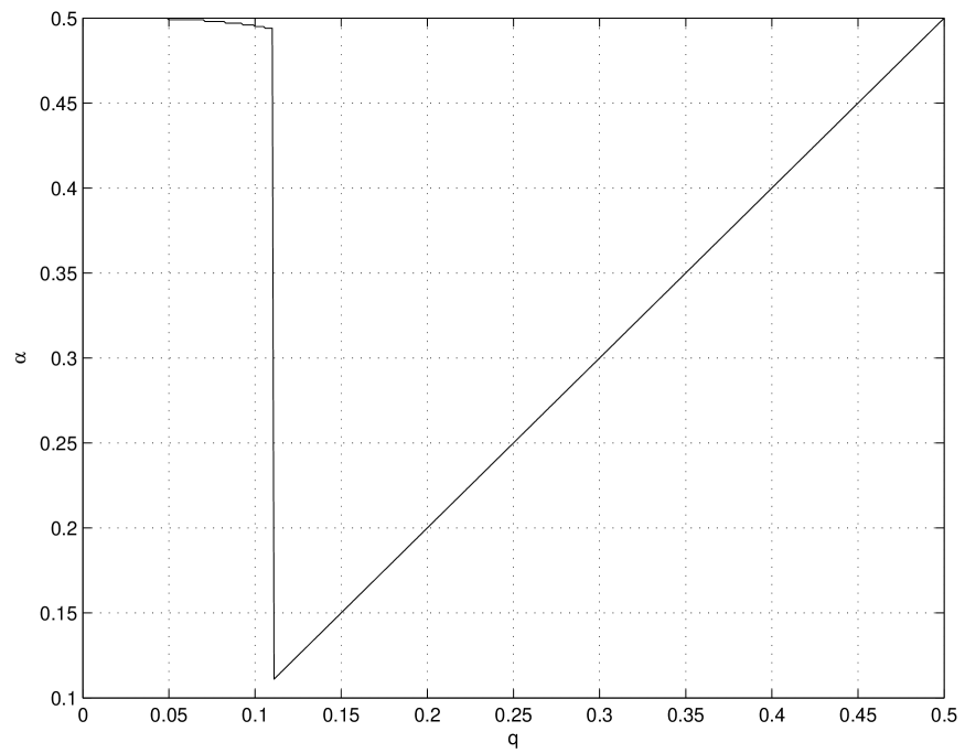
Note that in the first case () in (58) is achieved by , while in the third case () (58) is achieved by as shown in Fig. 5. Although, we do not have an explicit expression for in the range , the bound is sufficient for the purpose of proving Theorem 2 because . In Fig. 4 a numerical characterization of is plotted.
Proof.
Define
From the discussion above about the cases of equality in (65), Lemma 3 will follow by showing that is otherwise smaller, i.e.,
| (68) |
for all . It is easy to see that for the function is monotonically increasing with , and thus . For and , is increasing with and decreasing with , and thus . Clearly, from symmetry, also for and , . As a consequence, we have to show that (68) is satisfied only for . Likewise, in the sequel we may assume without loss of generality that .
The bound for the interval : in this case (68) is equivalent to the following bound
| (69) |
The LHS is lower bounded by
| (70) | |||
| (71) | |||
| (72) |
where (70) follows since ; (71) follows since ; (72) follows from Lemma 4 below.
The bound for the interval : in this case (68) is equivalent to the following bound
| (73) |
For fixed and , let us denote the RHS and the LHS of (73) as
The function is convex- in , since it is a composition of the function which is non-decreasing convex- in the range and the function which is convex- in [24]. Since is linear function in and is convex- function in , the bound (73) is satisfied if the interval edges ( and ) satisfy this bound. For , (73) holds since
For where , the bound (73) is satisfied since
| (74) | ||||
| (75) | ||||
| (76) | ||||
| (77) | ||||
| (78) | ||||
| (79) |
where (75) follows from Lemma 5 since , and since ;(76) follows since for and defined in (61), we have ; (77) follows since , thus ; (78) follows since is decreing in , thus for . Therefore, the bound (73) follows which completes the proof. ∎
Lemma 4.
For , the following inequality is satisfied
| (80) |
Proof.
Since , it is sufficient to show that is non-decreasing function in , i.e., for , therefore
| (81) |
Due to monotonicity of the log function (81) is equivalent to
| (82) |
where was defined in (60). Since by the definition of (61) , it follows that if , and in particular for , which implies (82) as desired. ∎
Lemma 5.
Let
| (83) |
where , and where . The maximum of is achieved by
| (84) |
Proof.
By differentiating with respect to and comparing to zero, we get that
| (85) |
thus maximizes since the second derivative is negative, i.e., . The lemma is followed since . ∎
We are now in a position to summarize the proof of Theorem 2.
Appendix C A simplified Outer Bound for the Sum Capacity in the Strong Interference Gaussian Case
Lemma 6.
The best known single-letter sum capacity (7) of the Gaussian doubly-dirty MAC (26) with power constraints , , and strong interferences () is upper bounded by
| (91) |
where is the upper convex envelope operation with respect to and , and . The supremum is over all such that is independent of , and
for .
Proof.
Let us define the following functions (corresponds to of (44))
| (92) |
The second function is the following maximization of (92) with respect to .
| (93) | ||||
Finally, we define the upper convex envelope of with respect to and :
| (94) |
Clearly if we take only the rate sum equation in (6) we get an outer bound on the best known single-letter region,
| (95) | |||
| (96) | |||
| (97) | |||
| (98) | |||
| (99) | |||
| (100) | |||
| (101) | |||
| (102) | |||
| (103) |
where (97) follows since where as ; (98) follows from the definition of the conditional entropy; (99) follows since and since ; (100) follows from the definition of the function (92), likewise (101) follows from the definition of the function (94), and since and from the definition
(102) follows from Jensen’s inequality since is a concave function; (103) follows from the input constraints where
| (104) |
The lemma follows since the upper bound (103) for the rate sum is now independent of and , hence it also bound the single-letter region . ∎
Acknowledgment
The authors wish to thank Ashish Khisti for earlier discussions on the binary case. The authors also would like to thank Uri Erez for helpful comments.
References
- [1] M. Costa, “Writing on dirty paper,” IEEE Trans. Information Theory, vol. IT-29, pp. 439–441, May 1983.
- [2] S. Gelfand and M. S. Pinsker, “Coding for channel with random parameters,” Problemy Pered. Inform. (Problems of Inform. Trans.), vol. 9, No. 1, pp. 19–31, 1980.
- [3] T. M. Cover and J. A. Thomas, Elements of Information Theory. New York: Wiley, 1991.
- [4] A. Somekh-Baruch, S. Shamai, and S. Verdu, “Cooperative encoding with asymmetric state information at the transmitters,” in Proceedings 44th Annual Allerton Conference on Communication, Control, and Computing, Univ. of Illinois, Urbana, IL, USA, Sep. 2006.
- [5] S. Kotagiri and J. N. Laneman, “Multiple access channels with state information known at some encoders,” IEEE Trans. Information Theory, July 2006, submitted for publication.
- [6] S. A. Jafar, “Capacity with causal and non-causal side information - a unified view,” IEEE Trans. Information Theory, vol. IT-52, pp. 5468–5475, Dec. 2006.
- [7] K. Marton, “A coding theorem for the discrete memoryless broadcast channel,” IEEE Trans. Information Theory, vol. IT–22, pp. 374–377, May 1979.
- [8] U. Erez, S. Shamai, and R. Zamir, “Capacity and lattice strategies for canceling known interference,” IEEE Trans. Information Theory, vol. IT-51, pp. 3820–3833, Nov. 2005.
- [9] R. Zamir, S. Shamai, and U. Erez, “Nested linear/lattice codes for structured multiterminal binning,” IEEE Trans. Information Theory, vol. IT-48, pp. 1250–1276, June 2002.
- [10] T. Philosof, A. Khisti, U. Erez, and R. Zamir, “Lattice strategies for the dirty multiple access channel,” in Proceedings of IEEE International Symposium on Information Theory, Nice, France, June 2007.
- [11] J. Korner and K. Marton, “How to encode the modulo-two sum of binary sources,” IEEE Trans. Information Theory, vol. IT-25, pp. 219–221, March 1979.
- [12] T. M. Cover and B. Gopinath, Open Problems in Communication and Computation. New York: Springer-Verlag, 1987.
- [13] I. Csiszar and J. Korner, Information Theory - Coding Theorems for Discrete Memoryless Systems. New York: Academic Press, 1981.
- [14] B. Nazer and M. Gastpar, “Computation over multiple-access channels,” IEEE Trans. Information Theory, vol. IT-53, pp. 3498–3516, Oct. 2007.
- [15] D. Krithivasan and S. S. Pradhan, “Lattices for distributed source coding: Jointly Gaussian sources and reconstruction of a linear function,” arXiv:cs.IT/0707.3461V1.
- [16] A. Khisti, “Private communication.”
- [17] R. G. Gallager, Information Theory and Reliable Communication. New York, N.Y.: Wiley, 1968.
- [18] G. Cohen, I. Honkala, S. Litsyn, and A. Lobstein, Covering Codes. Amsterdam, The Netherlands: North Holland Publishing, 1997.
- [19] R. Ahlswede and J. Korner, “Source coding with side information and a converse for the degraded broadcast channel,” IEEE Trans. Information Theory, vol. 21, pp. 629–637, 1975.
- [20] A. Wyner, “On source coding with side information at the decoder,” IEEE Trans. Information Theory, vol. IT-21, pp. 294–300, 1975.
- [21] T. Berger, Multiterminal Source Coding. New York: In G.Longo, editor, the Information Theory Approach to Communications, Springer-Verlag, 1977.
- [22] L. F. Wei and G. D. Forney, “Multidimensional constellation - part I: Introduction, figures of merit, and generalized cross constellations,” vol. 7, pp. 877–892, Aug. 1989.
- [23] A. Cohen and R. Zamir, “Entropy amplification property and the loss for writing on dirty paper,” IEEE Trans. Information Theory, To appear, April 2008.
- [24] S. Boyd and L. Vandenberghe, Convex Optimization. Cambridge: Cambridge University Press, 2004.