The role of time integration in energy conservation in Smoothed Particle Hydrodynamics fluid dynamics simulations
Abstract
The choice of a time integration scheme is a crucial aspect of any transient fluid simulation, and Smoothed-Particle Hydrodynamics (SPH) is no exception. The influence of the time integration scheme on energy balance is here addressed. To do so, explicit expressions allowing to compute the deviations from the energy balance, induced by the time integration scheme, are provided. These expressions, computed a posteriori, are valid for different integration methods. Besides, a new formulation that improves energy conservation by enhancing stability, based on an implicit integration scheme, is proposed. Such formulation is tested with the simulation of a two-dimensional non-viscous impact of two jets, with no artificial dissipation terms. To the best of our knowledge, this is the first stable simulation of a non-dissipative system with a weakly-compressible SPH method. A viscous case, the Taylor-Green vortex, has also been simulated. Results show that an implicit time integration scheme also behaves better in a viscous context.
keywords:
stability, time integration scheme, energy balance, SPH1 Introduction
Smoothed-Particle Hydrodynamics (SPH) is a meshfree numerical method in which continuum media are discretized as a set of particles, which move in a Lagrangian manner [1]. There is no doubt that its meshless nature is the feature which has drawn more attention to the model, that is indeed well suited to problems dominated by complex geometries, such as simulations involving free surface flow, or flows driven by large boundary displacements.
In addition to that, SPH is built starting from a relatively simple formulation that can be applied to a wide variety of physical phenomena. Indeed, even though the model was initially developed in astrophysics [2, 3], it quickly spread to other disciplines, including free surface flows [4], solid mechanics [5, 6] and geomaterial mechanics [7].
An interesting feature of SPH which has been traditionally considered one of its main benefits is the conservation of both momentum and energy. The claim that the method features exact energy conservation has been made several times in the past [8, 9, 10], although literature may also be found (e.g. [11]) where such conservation is shown to be linked to the accuracy of the time integration algorithm. Therefore, a clear line of investigation to improve the stability of the model comes from the analysis of the time integration scheme. Previous research on this topic has already shown promising results [12, 13, 14, 15, 16].
Indeed SPH has been widely criticized for characteristic instabilities, particularly in its weakly-compressible SPH (WC-SPH) incarnation, which is by far the most popular one. One of the most aggressive solutions to avoid stability issues of WC-SPH is to implement it within a rigorous incompressible formulation, leading to Incompressible-SPH (I-SPH) [17], a method that inherits some good stability features of more conventional CFD methods [18], at the expense of increased algorithm complexity.
Within the WC-SPH formulation, and probably motivated by the excellent energy conservation properties, some authors attributed the instabilities to spurious zero-energy modes [19, 20]. Lately, the focus has been set on tensile instability [21, 22, 23]. The first formulation designed to mitigate the pernicious effects of this instability was X-SPH, in which the velocity field is smoothed at each particle using information from its neighbors [21]. Along this line, some authors [22] analyzed the convolution kernel, culminating in the work by Dehnen and Aly [23], where it was demonstrated that Wendland kernels benefit particle packing.
Another methodology to deal with the tensile instability which is gaining popularity is the Particle Shifting Technique (PST), in which the particles’ positions are slightly modified at the end of each time step in order to preserve particle packing [18, 24, 25, 26, 27, 28]. Some authors who have dealt with tensile instabilities are moving to the so-called Total Lagrangian formalism [29], specially in solid dynamics [30, 31, 32].
A different line of investigation to improve stability has been the application of extra energy dissipation terms, the most straightforward one being artificial viscosity [1]. However, research quickly targeted mass conservation as well, by means of Shepard filtering. Afterwards, the addition of dissipation terms to the mass conservation equation has been investigated, resulting in the -SPH [33], and Riemann solvers-based schemes [34]. The relation between both formulations has been addressed in the past [35, 36].
In many of the research targeted at intrinsic instabilities just described, it is not yet clear how novel algorithms and formulations may affect the conservation properties of the method. It is not unreasonable to suggest that these studies have been circumvented due to the fact that the SPH community has traditionally regarded SPH as an exact energy conservation model, and the efforts have been accordingly directed towards solutions to known drawbacks of the method. For instance, an energy analysis of the -SPH term was conducted in Antuono et al. [37], demonstrating that it is intrinsically dissipating energy far from the boundaries. However, such energy dissipation is presented as a pernicious side effect of the model, a point which is not obvious, as discussed below. Similarly, Green and Peiró [38] examine energy conservation and partition between kinetic, potential, and compressible energies at the post-processing stage, in order to assess different models, for a long-duration simulation.
In Cercos-Pita et al. [39], violations of exact energy conservation were formally demonstrated for the first time. In such work, fluid extensions are considered, and extra energy terms are shown to appear due to interactions with the boundary. The investigation was also extended to other boundary formulations [40].
Surprisingly, although both the influence of the time integration scheme in the stability and the benefits of eventual extra energy dissipation have been already demonstrated, the role of the time integration scheme in the energy conservation has not been addressed in the literature yet. This paper is therefore devoted to this topic. For the sake of simplicity, we focus on the WC-SPH formulation for non-viscous fluids.
In order to analyze energy balance, spatial and time discretization are independently considered: the former will be presented in Section 2 and the latter in Section 3. They are combined afterwards in a total energy balance in Section 3.2. In Section 4 an implicit time integration scheme is proposed in order to improve energy conservation. Then, numerical experiments are carried out in Section 5, in order to support the theoretical findings. One of the simulations presented in this Section would be the first stable simulation of a non-dissipative system with a weakly-compressible SPH method (to the best of our knowledge.) The other is an application of this methodology to a viscous benchmark case. Finally, conclusions are presented in Section 6.
2 Spatial discretization
This section deals chiefly with spatial discretization. The SPH governing equations are introduced in Section 2.1. Power balance is discussed in Section 2.2, where contributions to energy variation are identified and separated.
2.1 SPH numerical model
Herein we focus on weakly compressible flows, even though similar analyses can be carried out for incompressible flows, or even for different physical phenomena. Hence, the governing equation for the evolution of density is the conservation equation:
| (1) |
where denotes SPH operators, and abusing the notation, any magnitude resulting from the application of the SPH methodology. In the equation above is the density of an arbitrary -th particle, and , its velocity.
The evolution of the velocity field is a discrete version of the Navier-Stokes momentum equation,
| (2) |
where is the pressure, the viscosity coefficient, the acceleration due to external forces, and the Shepard renormalization factor (see, for instance [41]). The extra term with the coefficient , which appears in this discrete version and is absent in the continuum, is explained below.
In WC-SPH, these equations are closed by an equation of state (EOS) relating pressure and density:
| (3) |
where is the background pressure, is the reference density, and the speed of sound in the fluid. The latter is customarily set to a value high enough that the fluid behaves almost as if incompressible.
Incidentally, it may be highlighted that every single SPH related operator can be split in 2 terms,
| (4) |
i.e., all SPH operators can be split in the effect of the interactions with other fluid particles and the interactions with the boundary. The latter may adopt a number of forms [40]. For the sake of simplicity, only the first, “bulk”, part of the operators is considered in the main body of this article, and boundary effects are deferred to A.
Regarding the viscous term , it may take several forms [42, 43], and may even include bulk viscosity [44]. As with boundary effects, we leave this term undefined, for the sake of simplicity and generality.
The momentum equation (2) differs from the traditional SPH formalism (as e.g. in the works of Monaghan [1] and Violeau [45]), by an extra term involving , whose form is:
| (5) |
where the mass of an arbitrary -th particle, is the value of kernel function for particles and , and . This term consistently vanishes in the continuum, but not in the discrete formulation of the equations, except for highly ordered particle distributions, such as those often set up at the beginning of a simulation. This form of momentum equation is introduced by Colagrossi et al. [26], where the consequences of such a term are thoroughly discussed.
Equations (1) and (2) feature discrete divergence and gradient operators. For these, anti-symmetric SPH operators and may be considered, of the form:
| (6) | ||||
| (7) |
which are consistent with an error.
If the value is set to in Eq. (2), the resulting equation is effectively equivalent to using the popular symmetric pressure gradient operator [1, 45]
| (8) |
This formulation has been already considered by Colagrossi et al. [26] in the context of setting an optimal initial particle distribution. A symmetric pressure gradient operator grants immediate linear and angular momentum conservation, as well as power conservation [46]. However, we prefer to keep this term and the anti-symmetric gradient operator as two distinct terms, since the interplay between the two will be crucial, as further discussed below. The symmetry properties of these operators also play a main role in multiphase flow simulations and free-surface modelling, as discussed by Colagrossi et al. [47].
Finally, even if a linear EOS is suggested in Eq. (3), other expressions have been traditionally accepted in SPH, provided this more general relationship holds:
| (9) |
2.2 SPH Power balance
Analyses of power balance in SPH have been carried out several times in the past, e.g.: [37, 40, 39]. Every time that the balance is revisited, new terms are included, and a better arrangement of the existing ones is proposed. In this work, power balance is critical, so its development is carried out from the basics in this section. Incidentally, it should be highlighted that in this work “power balance” refers to the instantaneous balance, which only depends on the spatial SPH operators, while “energy balance” involves the time integration scheme.
Thus, temporarily accepting the acceleration term computed in Eq. (2) as the actual rate of variation of the particle velocity, the following kinetic power term can be defined,
| (10) |
which is indeed the discrete version of the continuous kinetic power. This kinetic power can be conveniently split in several terms applying Eqs. (2) and (4),
| (11) | ||||
| (12) | ||||
| (13) | ||||
| (14) | ||||
| (15) |
The first three terms above, Eqs. (12-14), are just discrete versions of well known terms in fluid dynamics. To be precise: corresponds to the work due to pressure, , to the power due to the viscous forces, and to power from conservative external forces.
The extra term (15) is due to the operator, and obviously vanishes if . Paradoxically, the vanishing of this term is not beneficial for the numerical scheme [46]. This can be easily checked out by rearranging the work due to pressure, , as the power due to compressibility, as it is usually done in fluid dynamics. To this end, the following identity, which is often used in order to prove that the anti-symmetric divergence (6) and the symmetric gradient (8) operators are skew-adjoint [48, 37] can be invoked:
| (16) |
See B for a straightforward calculation that shows that any pair of gradient and divergence operators that satisfy this identity will lead to the conservation of mechanical energy.
Eq. (16) can be written in terms of the anti-symmetric gradient (5) as
| (17) |
Using the identity of Eq. (17) in the work due to pressure, Eq. (12), and applying mass conservation, Eq. (1), the work due to pressure can be subsequently rearranged as
| (18) | ||||
| (19) |
where is the power due to the compressibility.
Finally, all these terms may be introduced in the power balance, Eq. (18), which can then be rewritten
| (20) |
The term at the right hand side is an extra term, whose presence causes a lack of energy conservation (in addition to the term due to viscosity, which has a physical basis). Hence, it is possible to automatically ensure exact power balance if a symmetric pressure gradient operator () is chosen. In other words: the symmetric pressure gradient operator enables the model to non-physically exchange kinetic and compressibility energies, for the sake of total power conservation. Consistently, the same calculation for the conservation of mechanical energy referred to above will arrive at an expression that is not constant in general, unless . Such power conservation feature of the symmetric pressure gradient operator was already discussed by Monaghan [46].
3 Time discretization
After time discretization, the semi-discrete magnitudes, (discrete in space but continuous in time) lead to fully discretized magnitudes, , where the superindex indicates evaluation at the n-th time step. This may be achieved by a number of different time integration schemes. In particular, several ones have been implemented in the most popular codes, e.g. improved Euler [51], Verlet [52], and second-order Runge-Kutta [53]. The benefits and drawbacks of some of these integration schemes have been addressed in the past, mainly from the point of view of stability and time step size [12, 13, 14, 16].
The fact that the integration in time is numerically performed, naturally implies an error. The presence of such a deviation term has already been introduced in the past (see, among others, Monaghan [46] and Price [11]), although its analysis has always been left aside.
The purpose of this section is to provide analytical expressions to evaluate these residuals in the most general case.
3.1 Equivalent Euler time scheme
In order to analyze a general integration scheme, the actual variation rates are computed a posteriori. These variation rates are defined, within a time step, as
| (21) |
where is the time step.
According to this, we define
| (22) | ||||
| (23) |
Let us remark that the variation rates defined by (21), (22) and (23) can only be computed a posteriori, that is, after the flow fields at time are obtained by the actual time integration algorithm. Let us also point out that these variation rates serve as an analysis tool to asses the effect of the time integration scheme, but are not involved in the time integration itself.
With this in mind, an “equivalent Euler integration scheme” can be defined a posteriori. This “equivalent scheme” gives, within the n-th time step and using the rates defined by (21), the same result as the considered time integration scheme using the actual variation rates, given by the SPH equations, and applying the corresponding algorithm.
3.2 SPH total energy balance
Considering the total kinetic energy of the discrete system, at any time step,
| (24) |
we can write the rate of total kinetic energy variation during consecutive time steps as
| (25) |
Developing this term one gets
| (26) |
Substituting by its value, according to the equivalent Euler scheme, gives
| (27) |
Let us now compute the deviation of this power away from that of Eq. (10), caused by the errors in the velocity field due to the time integration scheme:
| (28) |
for any time . Substituting (27) and (10) in (28) we get
| (29) |
On the other hand, the velocities computed with the fully discretized SPH scheme do not agree with the ones resulting from solving the semidiscrete scheme, as the time integrations involve an error.
Furthermore, the SPH approximation of the derivative, for can be split into two terms:
| (30) |
where is the vector difference, at time , between the SPH and the Equivalent Euler a posteriori variation rates. According to this, (29) can be rewritten as
| (31) |
The two terms in the sum above represent, respectively:
-
1.
The error due to approximating by , due to considering each as the variation rate of during the time step.
-
2.
The error committed in the variation rate, as expressed by (30).
Let us now return to equation (20). It should be noticed that this energy balance is only valid if all the magnitudes involved are considered at the same time instant.
In order to evaluate the error using equation (29), we need to evaluate at some This is therefore, computationally, a suboptimal approach. On the other hand, this methodology can be applied to any time integration scheme.
In order to close the balance after applying Eq. (20), similar error terms should be defined for the power due to the compressibility. To that aim, let us examine the nature of equation (27). The variation rate of the kinetic Energy defined by that expression can be seen as an extended kinetic power, built from the discrete velocity field. In effect, that equation represents an exact evaluation of the kinetic power if we consider a linearly extended velocity field. Using the variation rate for the velocity defined by (23), we define:
| (32) |
with . In effect, equation (27) corresponds to the exact kinetic power of a set of particles, moving in the way described by the field (32), evaluated at .
Therefore, a way of building an error term for the power due to compressibility, , is to assume linearly extended fluid fields evaluated at . With that in mind, consider the following extended fields according to the variation rates defined by (22) (23):
| (33) | ||||
| (34) |
Therefore, defining
| (35) |
and inserting our definition for ,
| (36) |
finally yields
| (37) |
This allows to introduce a final balance:
| (38) |
where is a combined deviation term:
| (39) |
Again, all terms at right hand side of Eq. (38) have to be considered as extra terms that cause a deviation from constant energy. It is therefore patent that enters as an additional deviation term, whose expression depends on the particular time integration scheme.
4 Implicit time step to improve the energy conservation
As discussed, in order to achieve exact energy conservation it is mandatory that the term vanishes. The most straightforward approach would consist on making the separate sub-terms, , and , identically vanish particle-wise for some :
| (40) | ||||
| (41) |
Diferent strategies may be used in order to satisfy (40) and (41) or, at least, reduce the difference between the actual and the SPH variation rates. In [54], an interesting perspective, consisting on adapting the force computation accordingly to the time integration scheme, is proposed. Another approach would be to act over the integrator. Along that line, implicit methods may be proposed. It is a well known fact that implicit methots improve the stability of numerical integration of ODEs. Here, an implicit midpoint method is proposed These methods, as will be discussed below, start from a guess for a mid-point position, which is iteratively refined until some condition (in our case, the previous equations) is satisfied within some tolerance. On the other hand, larger time steps could be employed, thereby perhaps compensating the extra computational cost per time step, since implicit methods are known to have better stability features [55]. These aspects will be further discussed in the next section.
4.1 An implicit midpoint method
Regarding the time discretization, several schemes have been considered in this work:
-
1.
Explicit Euler scheme: it is the simplest integration scheme, in which values of the derivative at some time step are used to evaluate values at the next step. The scheme is first order and not A-stable. A-stability is a category of ODE solvers for which the solution is always stable, see [56].
- 2.
-
3.
Implicit midpoint method: a predictor-corrector scheme in which the mid point is guessed, and then iteratively refined. It is second order and A-stable.
In the particular case of the implicit midpoint method, the time in which the fields are evaluated is . In order to solve the implicit equation at every time step, a solution strategy must be defined, such as an iteration to find a fixed solution. To this end, initial guesses and for the velocity and density variation rates, respectively, are (we use superscripts as iteration indices):
| (42) | |||
| (43) |
which start an iterative process. The values of the extended velocity and density fields at each iteration are noted by and , respectively. The SPH approximations to these fields at each iterations are noted and . With this in mind, one has
| (44) | ||||
| (45) | ||||
| (46) | ||||
| (47) |
In the expressions above is the relaxation factor at iteration , which has been set to
| (48) |
where is the maximum number of iterations (either or , in this practical application), and a value tuned to get a small initial and final relaxation factor, .
5 Numerical verification
In order to focus only on compressibility and kinetic energies, a practical application based on the frontal impact of two jets has been selected. Results are described next, in Section 5.1. However, legitimate concerns may arise regarding the role of the implicit time-integration scheme on a viscous simulation. Thus, a simulation of the Taylor-Green Vortex has also been carried out, with results in Section 5.2.
5.1 Frontal jet impact
This practical application has already been considered in order to assess energy conservation in SPH by Marrone et al. [58].
The initial condition is schematically depicted in Fig. 1.

Two identical water jets of dimensions each, with the same constant velocity , but opposite directions, collide along the plane at the initial time instant, . Inviscid flow with a initially constant density field, , is considered for both jets. Also, no background pressure, , or volumetric forces, are considered. Thus, the whole phenomenon is characterized by the Mach number, .
When incompressible flow is considered, the impact causes a sudden loss of a fraction of the initial energy dependent on the parameters chosen [59]. Along this line, Marrone et al. [58] demonstrated that applying -SPH the simulation converges to the expected energy loss, while however not being an instantaneous process anymore. In contrast, in this paper an energy conserving impact is sought, in such a way that kinetic and compressibility energies are exchanged without any net loss, due to the lack of dissipative terms.
5.1.1 Numerical scheme
To carry out the simulations, dimensions are chosen, as well as reference density and initial velocity magnitude. No background pressure or volumetric forces are included: , . No extra dissipation is considered, either artificial viscosity or -SPH. The speed of sound is set at , as in Ref. [58], in order , so that the system is close to incompressible. Results are largely independent of this value as long as it is large enough. A parameter is set for all the simulations. Finally, the free-surface is modeled by straight compact support truncation [47].
The term has been dropped from the energy balance due to the parameter selection. However, is not vanishing by any means: indeed, that term is still able to trade kinetic and internal energy for the sake of exact total energy conservation, as discussed in Sec. 2.2.
The terms , Eq. (15), and , Eq. (39), do not have a clear sign. Thus, the corresponding residual are defined with absolute values:
| (50) | ||||
| (51) |
such that the total non-physical energy exchange may be quantified.
In a similar fashion, the following specific energy is defined as well,
| (52) |
The fluid domain is discretized in a lattice of particles with the same mass , resulting in an initial inter-particle spacing of . A quintic Wendland kernel [23] is applied, and its smoothing length is chosen so that .
5.1.2 Results
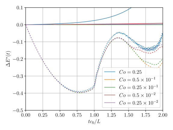
Pipelines with the numerical schemes described above have been implemented in the numerical package AQUAgpusph [51, 60, 61]. In Fig. 2 the energy evolution of the system is depicted for the explicit Euler scheme at different Courant numbers. This is defined as usual, Co=, where is the spatial spacing, which unless otherwise indicated is , with the total number of particles set to . The variation in energy is quantified by its relative change about its initial value
| (53) |
an expression used both for the total energy and the kinetic energy.
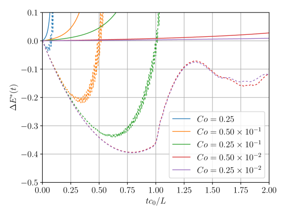
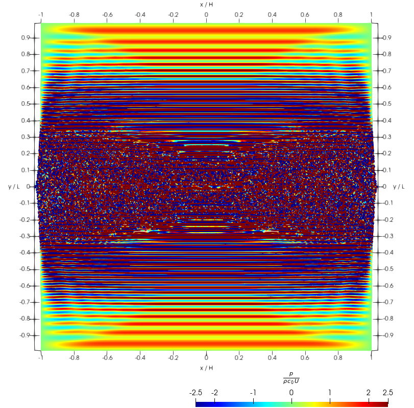
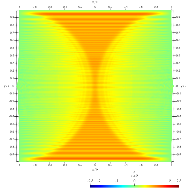
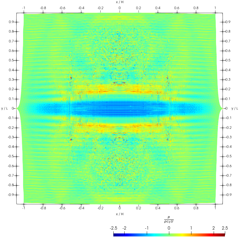
As can be appreciated, the simulation quickly turns unstable for large Courant numbers, . This is also seen in the simulation snapshots shown in Fig. 3, for the “impact time” . This particular time is important, since at this time the pressure shock-wave reaches the top and bottom boundaries. This shock-wave is then reflected as a second shock-wave traveling into the fluid domain, imploding at a time around , a time which will also be featured in our snapshots, and will be called “the second impact.”
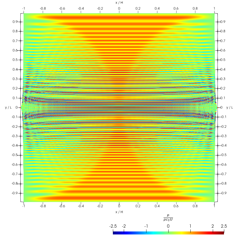
For smaller Courant numbers the total energy is much better conserved. Some energy is seen in Fig. 2 to be artificially pumped into the system anyway, and therefore, the stability of the simulation cannot be granted in the long run. Moreover, stability is compromised by early spatial instabilities, which resemble the well-known tensile instability. This is indicated by the kinetic energy behavior around the second impact (reduced time around ) in same Fig. 2, as well as in the snapshots shown in Fig. 4 for this time.
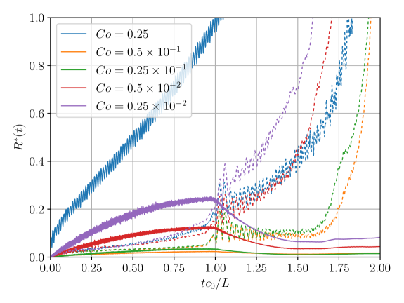
The effect of these instabilities is also highlighted in Fig. 5, where the residuals, , Eq. (50), and , , Eq. (51), are depicted along the simulation. For convenience, these are plotted in non-dimensional form,
| (54) |
since the residuals have dimensions of power.
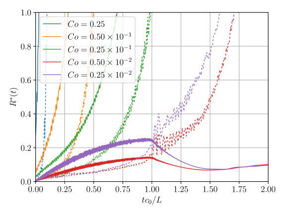
Indeed, for the three largest time steps the term quickly diverges, driving the instability. Even when the time step is low enough to avoid exponential total energy grow, the phenomenon seems to be dominated by at the early stages of the simulation. This trend changes after the shockwave reaches the top and bottom boundaries, at the impact time , when the residual term becomes the leading one. As the shockwave is reflected back into the fluid domain, negative pressure values appear, which have been widely associated with tensile instability in the past.
If the explicit Heun method is employed for these simulations, energy conservation is significantly improved, as can be seen in Fig. 6. Only the largest time step causes a significant amount of energy artificially pumped into the system.
Nevertheless, the simulation features trends similar to the explicit Euler method, as shown by the residuals plotted in Fig. 7. The simulations again are dominated by tensile instabilities after the shockwave reaches the top and bottom boundaries.
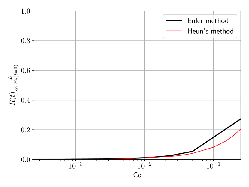
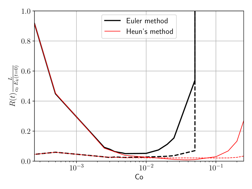
Both explicit time schemes have exposed consistency issues as the time step is decreased. In fact, in Figs. 5 and 7 residues do not seem vanish as the time step is made smaller. This is made clear in Fig. 8, where the residues at and are depicted for different Courant numbers. Indeed, at the first time step both residues vanish as the time step is diminished, which is not however the case after a short time lapse. The minima in the residues clearly shows an optimal value for the time step, for each time integration scheme. Further reductions of the time step size inexorably lead to worse energy conservation. Consistently, the difference between both integration schemes is negligible for the smallest Courant numbers.
Employing the implicit midpoint method, the energy and residues evolution depicted in Figs. 9 and 10 are obtained.
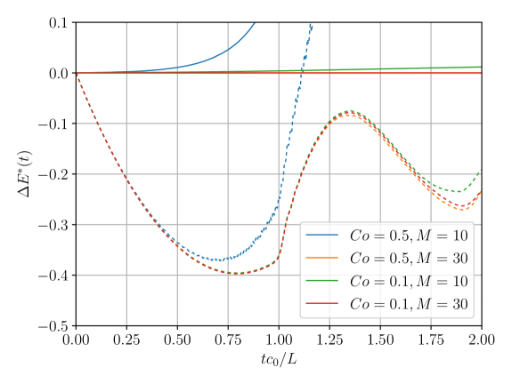
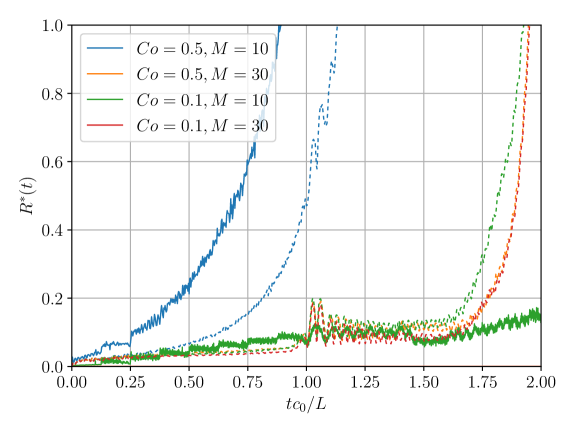
Even for the largest time step, good total energy conservation can be achieved when iterations are considered to solve the fixed point problems. Furthermore, it can be appreciated that an increase in the number of iterations computationally outperforms a reduction of the Courant number.
A more quantitative approach is to describe the number of numerical iterations, #s, needed in order to evolve the simulation to a given time. The main point is that each iteration has nearly the same computational cost for the explicit and implicit methods, and, while the actual running time will depend on the architecture used, the number of iterations will not. Some estimates of these numbers are now discussed, since we think that an in-deep analysis of computational cost is not so useful for the idealized test cases in this work.
In general, , which in terms of the Courant number can be written as .
In most of the simulations of the frontal jet impact of Sec. 5.1, the number of particles is , and since , we simply have , where is the physical time, and the number of inner iterations ( for explicit methods). This way, results for the explicit Euler scheme in Figs. 2 and 5 show that about iterations are needed in order to obtain acceptable results at the impact time (.) This number is greatly reduced, to about , in the Heun method, as seen in Figs. 6 and 7. These two values are actually close to the optimum ones at in Fig. 8 (b), namely for the explicit Euler scheme, and for Heun method.
The implicit midpoint method, with results in Figs. 9, 10, and 11, seem to require about iterations. According to this metrics, it would then seem that certain explicit methods are actually preferable to our implicit proposal.This is not the case in the next simulation case, the Taylor-Green vortex, as will be discussed in section 5.2.
Despite the significantly better energy conservation, the residue associated with a spatial instability, , is inconsistently converging to a non-zero value when either the time step is decreased or the number of iterations is increased. A large amount of internal and kinetic energy is artificially exchanged by this term at the second impact, for all considered Courant numbers and number of iterations. Such non-physical energy exchange can be however diminished by including more particles, as can be seen in Fig. 11, where the residues are plotted for a varying number of particles, , at constant Courant number , and iterations. Negligible total energy residues, , are consistently obtained for all the simulations. This permits these simulations to run for long times, without breaking down at the early stages. The figure also features preliminary results from a Particle Shifting Technique which will be briefly described in Sec. 7, and show an even better evolution of the residues.
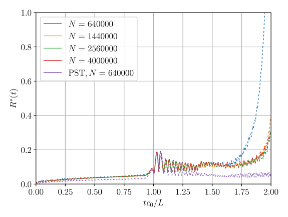
Nevertheless, the term is not converging to zero, either in time or in space. This, is in fact, expected due to the inconsistencies related to the free-surface, as already described by Colagrossi et al. [47].
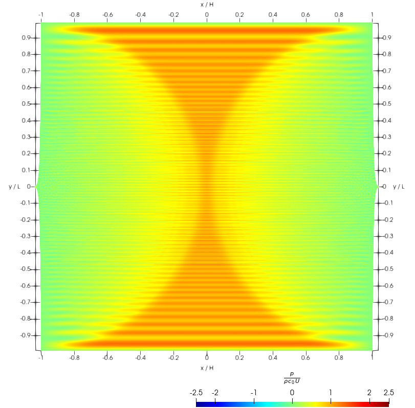
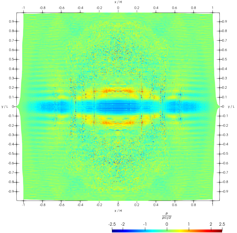
In Fig. 12 the specific internal and kinetic energy artificially traded is depicted for each particle, at the second impact time .
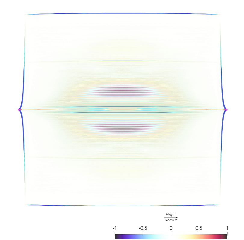
A significant amount of kinetic energy is indeed non-physically transformed into internal energy close to the free-surface. However, artificially exchanged energy can also be found far away from the free-surface, specially close to the impact line, where largest negative pressure values occur.
5.2 Taylor-Green vortex
The Taylor-Green Vortex [62] is a popular practical application in which vortices are simulated in a periodic domain. The initial condition is schematically depicted in Fig. 13.

A square domain of size contains four counter-rotating vortices, described by the initial velocity field
| (55) | ||||
where is the characteristic velocity. Periodic boundary conditions are considered.
The corresponding pressure field is
| (56) |
with areplacednd the reference density and background pressure. The time evolution is analytically solvable, with the same expressions as above, but with replaced by , where is the kinematic viscosity coefficient.
In this particular case a Reynolds number, , is chosen. As discussed below, larger Reynolds numbers can safely be considered when the implicit time integrator is applied. However, increasing the Reynolds number for the Euler explicit time scheme would require a extremely large number of particles, as well as an extremely small time step.
5.2.1 Numerical scheme
To carry out the simulations, , and parameters are selected. No volumetric forces are included, . However, in contrast to the previous practical application, a non-null background pressure is considered, . The speed of sound is set at , resulting in a .
The particles are distributed in a lattice grid, with particles along both the and direction. That makes a total of particles, with initial inter-particle spacing . At the beginning of the simulation, the particles in the spaces between vortices will compress in one direction and expand in the other. Therefore, an anisotropic distribution of particles will be obtained, which will make the simulation unstable unless the kernel length is large enough. With the choice of the inter-particle distance over smoothing length ratio made in this particular example, , it follows that the value representing the artificial viscosity, see [1, 46], is
| (57) |
a value usually considered low enough to get stable simulations.
For the sake of simplicity, during this practical simulation only the explicit Euler scheme and the implicit midpoint method are discussed. Indeed, due to the required small time steps, the differences between the explicit Heun method and the Euler one have been seen to be negligible.
5.2.2 Results
Simulations are again carried out by the numerical package AQUAgpusph [61, 51, 60]. In Fig. 14 the energy evolution of the system is depicted for the explicit Euler scheme at different Courant numbers, as well as the implicit time integrator in a unique configuration. The variation in energy is again quantified by its relative change about its initial value. The total energy includes the kinetic and potential energies, plus the energy dissipated by viscosity (in absolute value), hence its value should remain constant.
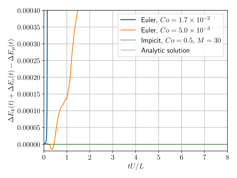
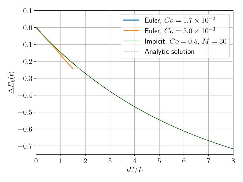
As can be appreciated, the implicit midpoint method is able to conserve the total energy of the system for a long time, while capturing the kinetic energy decay phenomena predicted by the analytic solution [62]. Conversely, when the explicit Euler scheme is considered, a Courant number would quickly result in an unstable simulation, with poor energy conservation and an overestimated viscous dissipation. Therefore it can be asserted that the implicit midpoint method is able to outperform the explicit schemes.
As analyzed for the previous case, if we compare results for numerical iterations at (see Fig. 14), we find the following: the explicit scheme needs about steps for the higher Courant number, and for the lower one, while the implicit scheme needs , i.e. with a number of iterations similar to the coarser explicit scheme, the implicit methods provide much better results. For greater times, the explicit results become much less accurate. For these simulations, particles are used, , and , so
The simulation is stable for slightly longer if a extremely small Courant number is considered, . In such case, the explicit Euler scheme is able to keep the energy well conserved for the first half of spin. Unfortunately it is not able to keep it up, so at the end of the first spin the scheme is already pumping spurious energy in a constant basis. Those energy conservation flaws induce instabilities, as can be appreciated in Fig. 15.
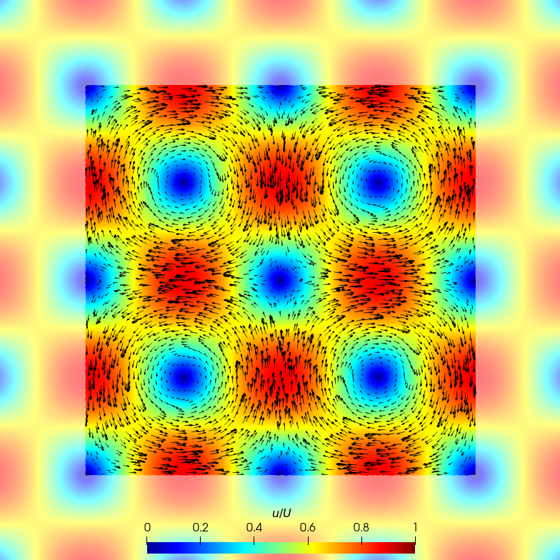
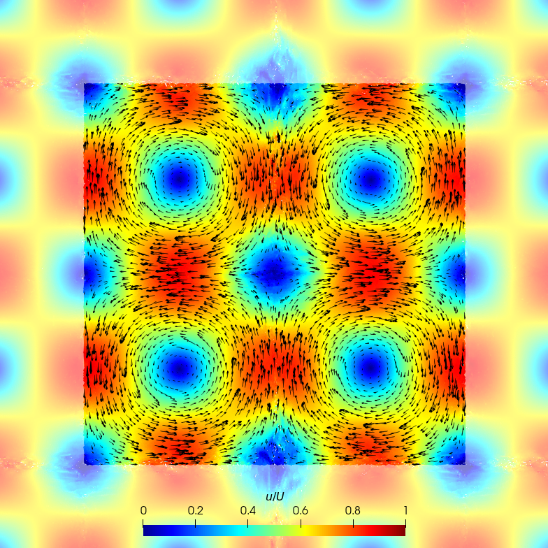
These noisy fields consequently result in larger kinetic energy dissipation that can be appreciated in Fig. 14.
Thus, it can be asserted that the implicit midpoint method does not play a role in the viscous term itself, either implying extra numerical dissipation or the inverse. However, the time integration scheme is indirectly related to viscous dissipation through the noise on the resulting fields. Along this line, an explicit scheme artificially pumping energy in the system will inexorably result in larger viscous dissipation.
6 Conclusions
The instantaneous SPH power balance for fluid dynamics has been revisited. A new power term, associated to spatial instabilities, has been added to the balance. It has been demonstrated that such term, which was formerly considered as part of the work flow term, can trade kinetic and internal energy, in a non-physical fashion, for the sake of total instantaneous power conservation.
In addition to the improvements on instantaneous power balance, the role of the time integration scheme on the energy balance has also been investigated. It is demonstrated that energy conservation cannot be granted with explicit time integration schemes, while an implicit midpoint method produces good results (it is likely that other implicit methods are successful in this regard.) A framework to track the errors on the energy conservation has been discussed, which may be applied to assessing the quality of simulation results, and to tuning extra dissipation models, like artificial viscosity or -SPH.
Simulations of the frontal impact of non-viscous 2-D jets have been carried out. Non-negligible total energy conservation errors are obtained for all the simulations when either Euler or Heun explicit time integration schemes are considered. For these, reducing the time step will not monotonically reduce total energy conservation errors, but a minimum error is obtained, for an optimal time step, which depends on the specific scheme. On the other hand, when the implicit midpoint method is considered, with inner iterations, negligible total energy conservation errors are obtained, even for large Courant numbers.
Having a look at the number of numerical iterations needed to evolve a simulation to a certain time, the performance of explicit and implicit methods depends on the simulated case. For the inviscid impact test done in the present work, some explicit methods need a smaller number of iterations than the proposed implicit scheme. However, for a case including viscosity, such as the Taylor-Green vortex tested here, the implicit method shows a better performance.
Regarding stability, all methods considered fail for the frontal jet impact, the explicit ones around the time of the second impact, and the implicit one around the third one. Preliminary results with a PST show long-term stability for the latter method. For the Taylor-Green vortex, the explicit schemes fail rather quickly, whereas the implicit method is stable throughout the simulation.
From a point of view purely centered in practical applications, this is (in our opinion) an important step towards stable WC-SPH simulations, in systems with no extra energy dissipation. In contrast with previous simulations, in this work kinetic and internal energy are continuously traded as the shockwave travels from the impact front to the fluid edges and back. This leads to simulations that can run for a long time.
The pipelines implemented to carry out the simulations in the SPH solver AQUAgpusph can be found at the project’s website [61].
7 Future work
Although the theoretical analysis may be extended in a straightforward way in order to include energy exchange through the boundaries (see A), a practical application in which all those terms are vanishing has been selected. This is because a wide variety of boundary conditions and formulations should have been otherwise considered. In addition to that, this energy exchange has already been covered in the literature, with the exception of the term , Eq. (60), an artificial energy exchanged with the boundary which deserves further analysis.
A framework to compute deviations away from total energy conservation has been presented, and applied in our simulations. However, such framework can be potentially considered to tune extra dissipation terms, like artificial viscosity or -SPH, while still applying explicit time integration schemes. The performance of such approach may be further analyzed in future works.
The simulations show that energy conservation is not converging as the Courant number is reduced, for the explicit time integration schemes. The roots of that counter-intuitive trend has not been addressed in detail, and should therefore be analyzed in future publications.
A clear avenue for improvement would the alleviation of spatial instabilities, obvious e.g. in Fig. 3, perhaps through some particle-shifting technique (PST). In this regard, Fig. 11 includes (PST) preliminary results that show a great reduction in the residues, that persists for long simulation times. Details of this PST will shortly be published in a separate article.
Acknowledgments
This work has been partially supported by the Swedish Research Council, under grant 2018-02438, and the Ministry of Science, Innovation, and Universities, under research project RTI2018-096791-B-C21, Hydrodynamics of Motion Damping Devices for Floating Offshore Wind Turbines (FOWT-DAMP). P.E. Merino is supported during the completion of his Ph.D. thesis by MEyFP grant FPU17/05433 and thanks MEyFP for its support.
Data availability
The data that support the findings of this study are available from the corresponding author upon reasonable request.
Appendix A Boundaries
As mentioned in Eq. (4), every single SPH related operator can be split in a bulk term and a boundary term.
As a consequence, Eq. (11) would read, in general,
| (58) |
where the bulk terms are now explicitly marked with an superscript, and two new boundary terms appear. One corresponds to the discrete version of the mechanical work done by the boundaries upon the fluid:
| (59) |
while the other is due to the operator:
| (60) |
Eq. (18) likewise has an extra term:
| (61) |
where
| (62) |
is the work exerted by the boundaries on the fluid due to compressibility, already discussed in Cercos-Pita et al. [39].
Finally, Eq. (20), now reads
| (63) | ||||
| (64) |
Again, all the terms at the right hand side this equation are extra terms, whose presence causes a lack of energy conservation. Conservation is enforced in this work by setting , and by considering no boundaries.
The extra work term, , has been already analyzed in previous works [40, 39]. On the other hand, the extra work term is new, as it has been traditionally considered part of . However, the latter term has a purely numerical nature, and should be therefore split, yielding such an extra term.
It is interesting now to recall the work of Mayrhofer et al. [48], where the possibility of getting and skew-adjoint operators was analyzed within the boundary integrals formulation. A methodology to achieve that was even proposed therein, but never tested. It would be therefore interesting to revisit that work to further analyze the relation between the terms and . This is however not pursued in this paper, as that will exceed its scope and make it too lengthy.
Appendix B Conservation of energy
We briefly show that any two gradient and divergence operators satisfying skew-adjointness property (Eq. (16)) will lead to the mechanical energy being conserved in the absence of viscosity. In Colagrossi et al. [47] an application of this property within a continuum SPH context can be found.
Euler’s momentum equation is (2), neglecting and (the latter, for the sake of simplicity). Considering first , it reads
Applying , and summing over all particles,
This may be written as
where is the total kinetic energy. (In this derivation, time derivatives are supposed to satisfy the usual rules of calculus. This is a subtle point on which we do not have space to dwell here.)
Thanks to skew-adjointness,
Now the appearance of the divergence reminds us of continuity, Eq. (1), from which
Therefore,
Then, defining the total internal energy
We find
expressing the fact that the mechanical energy, , does not change. If value different than is considered, the final expression is not seen to conserve energy in general. For reference, the final expression using our antisymmetric operators is
If , the term inside the square brackets simplifies
and the continuity equation may be used in order to deduce energy conservation.
Appendix C Consequences of a -SPH model
We briefly discuss, for convenience to interested readers, the modifications that a -SPH formulation would bring about.
In this framework, the conservation Eq. (1) has an extra term:
| (66) |
whose specific shape we leave unspecified, for the sake of generality.
Eq. (58) does not change, but Eq. (63) does:
| (67) |
where the dots represent, again for simplicity, the part of Eq. (63) that has not changed, and:
| (68) |
I.e. the -SPH term gives rise to the first, bulk power, term, [37] and the second term, related to the energy exchanged through the boundaries.
Antuono et al. [37] previously merged and into a single term, but we propose it should be split. This allows to relax the conditions imposed on , in such a way that the theoretical analysis in that work becomes valid — in particular, the fact that the term leads to energy dissipation, therefore contributing to the stability of the model. They also analyzed numerically the overall contribution from both terms, checking that they were not pumping energy in the system, so it can be expected that the effect of the term is negligible. A formal analysis is still required though.
References
- Monaghan [2012] J. J. Monaghan, Smoothed Particle Hydrodynamics and Its Diverse Applications, Annual Review of Fluid Mechanics 44 (2012) 323–346.
- Lucy [1977] L. Lucy, A numerical approach to the testing of the fission hypothesis, Astronomical Journal 82 (1977) 1013–1024.
- Gingold and Monaghan [1977] R. Gingold, J. J. Monaghan, Smoothed Particle Hydrodynamics: theory and application to non-spherical stars, Mon. Not. Roy. Astron. Soc. (MNRAS) 181 (1977) 375–389.
- Monaghan [1994] J. J. Monaghan, Simulating Free Surface Flows with SPH, J. Comp. Phys. 110 (1994) 39–406.
- Rabczuk and Eibl [2003] T. Rabczuk, J. Eibl, Simulation of high velocity concrete fragmentation using SPH/MLSPH, International Journal for Numerical Methods in Engineering 56 (2003) 1421–1444.
- Bonet et al. [2004] J. Bonet, S. Kulasegaram, M. Rodriguez-Paz, M. Profit, Variational formulation for the smooth particle hydrodynamics (SPH) simulation of fluid and solid problems, Computer Methods in Applied Mechanics and Engineering 193 (2004) 1245–1256.
- Bui et al. [2008] H. H. Bui, R. Fukagawa, K. Sako, S. Ohno, Lagrangian meshfree particles method (SPH) for large deformation and failure flows of geomaterial using elastic–plastic soil constitutive model, International Journal for Numerical and Analytical Methods in Geomechanics 32 (2008) 1537–1570.
- Monaghan and Gingold [1983] J. J. Monaghan, R. A. Gingold, Shock simulation by the particle method SPH, Journal of computational physics 52 (1983) 374–389.
- Couchman and Thomas [1995] H. Couchman, P. Thomas, Hydra: An adaptative-mesh implementation of (1995).
- Vaughan et al. [2008] G. Vaughan, T. R. Healy, K. R. Bryan, A. D. Sneyd, R. Gorman, Completeness, conservation and error in SPH for fluids, International journal for numerical methods in fluids 56 (2008) 37–62.
- Price [2008] D. J. Price, Modelling discontinuities and Kelvin–Helmholtz instabilities in SPH, Journal of Computational Physics 227 (2008) 10040–10057.
- Dyka et al. [1997] C. Dyka, P. Randles, R. Ingel, Stress points for tension instability in SPH, International Journal for Numerical Methods in Engineering 40 (1997) 2325–2341.
- Rook et al. [2007] R. Rook, M. Yildiz, S. Dost, Modeling transient heat transfer using SPH and implicit time integration, Numerical Heat Transfer, Part B: Fundamentals 51 (2007) 1–23.
- Colagrossi et al. [2010] A. Colagrossi, C. Lugni, M. Brocchini, A study of violent sloshing wave impacts using an improved SPH method, Journal of hydraulic research 48 (2010) 94–104.
- Blanc and Pastor [2012] T. Blanc, M. Pastor, A stabilized fractional step, Runge-Kutta Taylor SPH algorithm for coupled problems in geomechanics, Computer Methods in Applied Mechanics and Engineering 221-222 (2012) 41 – 53.
- Mabssout and Herreros [2013] M. Mabssout, M. Herreros, Runge–Kutta vs Taylor-SPH: Two time integration schemes for SPH with application to Soil Dynamics, Applied Mathematical Modelling 37 (2013) 3541–3563.
- Cummins and Rudman [1999] S. J. Cummins, M. Rudman, An SPH Projection Method, Journal of Computational Physics 152 (1999) 584–607.
- Xu et al. [2009] R. Xu, P. Stansby, D. Laurence, Accuracy and stability in incompressible SPH (ISPH) based on the projection method and a new approach, Journal of Computational Physics 228 (2009) 6703–6725.
- Vignjevic et al. [2000] R. Vignjevic, J. Campbell, L. Libersky, A treatment of zero-energy modes in the smoothed particle hydrodynamics method, Computer methods in Applied mechanics and Engineering 184 (2000) 67–85.
- Vidal et al. [2007] Y. Vidal, J. Bonet, A. Huerta, Stabilized updated Lagrangian corrected SPH for explicit dynamic problems, International journal for numerical methods in engineering 69 (2007) 2687–2710.
- Monaghan [2000] J. J. Monaghan, SPH without a tensile instability, J. Comp. Phys. 159 (2000) 290–311.
- Swegle et al. [1995] J. W. Swegle, D. L. Hicks, S. W. Attaway, Smoothed Particle Hydrodynamics Stability Analysis, Journal of Computational Physics 116 (1995) 123–134.
- Dehnen and Aly [2012] W. Dehnen, H. Aly, Improving convergence in smoothed particle hydrodynamics simulations without pairing instability, Monthly Notices of the Royal Astronomical Society 425 (2012) 1068–1082.
- Lind et al. [2012] S. J. Lind, R. Xu, P. K. Stansby, B. D. Rogers, Incompressible smoothed particle hydrodynamics for free-surface flows: A generalised diffusion-based algorithm for stability and validations for impulsive flows and propagating waves, Journal of Computational Physics 231 (2012) 1499–1523.
- Vacondio et al. [2013] R. Vacondio, B. Rogers, P. Stansby, P. Mignosa, J. Feldman, Variable resolution for SPH: a dynamic particle coalescing and splitting scheme, Computer Methods in Applied Mechanics and Engineering (2013).
- Colagrossi et al. [2012] A. Colagrossi, B. Bouscasse, M. Antuono, S. Marrone, Particle packing algorithm for SPH schemes, Computer Physics Communications 183 (2012) 1641–1683.
- Oger et al. [2016] G. Oger, S. Marrone, D. Le Touzé, M. De Leffe, Sph accuracy improvement through the combination of a quasi-lagrangian shifting transport velocity and consistent ale formalisms, Journal of Computational Physics 313 (2016) 76–98.
- Sun et al. [2019] P. Sun, A. Colagrossi, S. Marrone, M. Antuono, A.-M. Zhang, A consistent approach to particle shifting in the -Plus-SPH model, Computer Methods in Applied Mechanics and Engineering 348 (2019) 912–934.
- Vignjevic et al. [2006] R. Vignjevic, J. R. Reveles, J. Campbell, SPH in a total lagrangian formalism, CMC-Tech Science Press- 4 (2006) 181.
- Bonet and Kulasegaram [2002] J. Bonet, S. Kulasegaram, Alternative total lagrangian formulations for corrected smooth particle hydrodynamics (CSPH) methods in large strain dynamic problems, Revue Européenne des Éléments Finis 11 (2002) 893–912.
- Zhang et al. [2014] A. Zhang, F. Ming, X. Cao, Total Lagrangian particle method for the large-deformation analyses of solids and curved shells, Acta Mechanica 225 (2014) 253–275.
- Islam and Peng [2019] M. R. I. Islam, C. Peng, A Total Lagrangian SPH method for modelling damage and failure in solids, International Journal of Mechanical Sciences 157 (2019) 498–511.
- Antuono et al. [2012] M. Antuono, A. Colagrossi, S. Marrone, Numerical diffusive terms in weakly-compressible SPH schemes, Computer Physics Communications 183 (2012) 2570–2580.
- Vila [1999] J. Vila, On particle weighted methods and Smooth Particle Hydrodynamics, Mathematical Models & Methods in Applied Sciences 9 (1999) 161–209.
- Cercos-Pita et al. [2016] J. Cercos-Pita, R. Dalrymple, A. Herault, Diffusive terms for the conservation of mass equation in SPH, Applied Mathematical Modelling 40 (2016) 8722 – 8736.
- Green et al. [2019] M. D. Green, R. Vacondio, J. Peiró, A smoothed particle hydrodynamics numerical scheme with a consistent diffusion term for the continuity equation, Computers & Fluids 179 (2019) 632–644.
- Antuono et al. [2015] M. Antuono, S. Marrone, A. Colagrossi, B. Bouscasse, Energy balance in the -SPH scheme, Computer Methods in Applied Mechanics and Engineering 289 (2015) 209–226.
- Green and Peiró [2018] M. D. Green, J. Peiró, Long duration SPH simulations of sloshing in tanks with a low fill ratio and high stretching, Computers & Fluids 174 (2018) 179–199.
- Cercos-Pita et al. [2017] J. Cercos-Pita, M. Antuono, A. Colagrossi, A. Souto-Iglesias, SPH energy conservation for fluid–solid interactions, Computer Methods in Applied Mechanics and Engineering 317 (2017) 771–791.
- Cercos-Pita [2016] J. L. Cercos-Pita, A novel generalized diffusive SPH model: Theoretical analysis and 3D HPC implementation, Ph.D. thesis, Technical University of Madrid (UPM), 2016.
- Calderon-Sanchez et al. [2019] J. Calderon-Sanchez, J. Cercos-Pita, D. Duque, A geometric formulation of the shepard renormalization factor, Computers & Fluids 183 (2019) 16–27.
- Monaghan [1992] J. J. Monaghan, Smoothed Particle Hydrodynamics, Annual Review of Astronomy and astrophysics 30 (1992) 543–574.
- Morris and Monaghan [1997] J. Morris, J. J. Monaghan, A switch to reduce SPH viscosity, J. Comp. Phys. 136 (1997) 41–50.
- Avalos et al. [2020] J. B. Avalos, M. Antuono, A. Colagrossi, A. Souto-Iglesias, Shear-viscosity-independent bulk-viscosity term in smoothed particle hydrodynamics, Phys. Rev. E 101 (2020) 013302.
- Violeau [2012] D. Violeau, Fluid Mechanics and the SPH Method, Oxford University Press, 2012.
- Monaghan [2005] J. J. Monaghan, Smoothed particle hydrodynamics, Reports on Progress in Physics 68 (2005) 1703–1759.
- Colagrossi et al. [2009] A. Colagrossi, M. Antuono, D. Le Touzé, Theoretical considerations on the free-surface role in the smoothed-particle-hydrodynamics model, Physical Review E 79 (2009) 056701.
- Mayrhofer et al. [2013] A. Mayrhofer, B. D. Rogers, D. Violeau, M. Ferrand, Investigation of wall bounded flows using SPH and the unified semi-analytical wall boundary conditions, Computer Physics Communications 184 (2013) 2515–2527.
- Bonet and Lok [1999] J. Bonet, T.-S. Lok, Variational and momentum preservation aspects of smooth particle hydrodynamic formulations, Computer Methods in Applied Mechanics and Engineering 180 (1999) 97–115.
- Sun et al. [2018] P. Sun, A. Colagrossi, S. Marrone, A. Zhang, Multi-resolution -plus-SPH with tensile instability control: Towards high reynolds number flows, Computer Physics Communications 224 (2018) 63–80.
- Cercos-Pita [2015] J. Cercos-Pita, AQUAgpusph, a new free 3D SPH solver accelerated with OpenCL, Computer Physics Communications 192 (2015) 295–312.
- Crespo et al. [2015] A. Crespo, J. Dominguez, B. Rogers, M. Gomez-Gesteira, S. Longshaw, R. Canelas, R. Vacondio, A. Barreiro, O. Garcia-Feal, DualSPHysics: Open-source parallel CFD solver based on Smoothed Particle Hydrodynamics (SPH), Computer Physics Communications 187 (2015) 204–216.
- Herault et al. [2010] A. Herault, G. Bilotta, R. A. Dalrymple, SPH on GPU with CUDA, Journal of Hydraulic Research 48 (2010) 74–79.
- LaBudde and Greenspan [1974] R. A. LaBudde, D. Greenspan, Discrete mechanics—a general treatment, Journal of Computational Physics 15 (1974) 134–167.
- Leimkuhler and Reich [2005] B. Leimkuhler, S. Reich, Simulating Hamiltonian Dynamics, Cambridge Monographs on Applied and Computational Mathematics, Cambridge University Press, 2005. doi:10.1017/CBO9780511614118.
- Süli and Mayers [2003] E. Süli, D. Mayers, An Introduction to Numerical Analysis, Cambridge University Press, 2003. URL: https://books.google.es/books?id=hj9weaqJTbQC.
- Burden et al. [2015] R. Burden, J. Faires, A. Burden, Numerical Analysis, Cengage Learning, 2015. URL: https://books.google.es/books?id=9DV-BAAAQBAJ.
- Marrone et al. [2015] S. Marrone, A. Colagrossi, A. Di Mascio, D. Le Touzé, Prediction of energy losses in water impacts using incompressible and weakly compressible models, Journal of Fluids and Structures 54 (2015) 802–822.
- Szymczak [1994] W. Szymczak, Energy losses in non-classical free surface flows, in: J. Blake, J. Boulton-Stone, N. Thomas (Eds.), Bubble Dynamics and Interface Phenomena, volume 23 of Fluid Mechanics and Its Applications, Springer Netherlands, 1994, pp. 413–420. doi:10.1007/978-94-011-0938-3.
- Cercos-Pita et al. [2019] J. L. Cercos-Pita, J. Calderon-Sanchez, D. Duque, A Visual Block-Based SPH programming editor, in: 13th International SPHERIC SPH Workshop, 2019.
- AQU [2022] AQUAgpusph web site, http://canal.etsin.upm.es/aquagpusph, 2022.
- Taylor and Green [1937] G. I. Taylor, A. E. Green, Mechanism of the production of small eddies from large ones, Proceedings of the Royal Society of London. Series A-Mathematical and Physical Sciences 158 (1937) 499–521.