The shock formation and optimal regularities of the resulting shock curves for 1-D scalar conservation laws

Yin Huicheng^1,∗, Zhu Lu^2, ¹¹1Yin Huicheng (huicheng@nju.edu.cn, 05407@njnu.edu.cn) and Zhu Lu (zhulu@hhu.edu.cn) are supported by the NSFC (No.11571177, No.11731007, No.12001162).
1. School of Mathematical Sciences and Institute of Mathematical Sciences,
Nanjing Normal University, Nanjing, 210023, China.
2. College of Science, Hohai University, Nanjing, 210098, China

Abstract

The study on the shock formation and the regularities of the resulting shock surfaces for hyperbolic conservation laws is a basic problem in the nonlinear partial differential equations. In this paper, we are concerned with the shock formation and the optimal regularities of the resulting shock curves for the 1-D conservation law $\partial_{t}u+\partial_{x}f(u)=0$ with the smooth initial data $u(0,x)=u_{0}(x)$ . If $u_{0}(x)\in C^{1}(\mathbb{R})$ and $f(u)\in C^{2}(\mathbb{R})$ , it is well-known that the solution $u$ will blow up on the time $T^{*}=-\frac{1}{\min{g^{\prime}(x)}}$ when $\min{g^{\prime}(x)}<0$ holds for $g(x)=f^{\prime}(u_{0}(x))$ . Let $x_{0}$ be a local minimum point of $g^{\prime}(x)$ such that $g^{\prime}(x_{0})=\min{g^{\prime}(x)}<0$ and $g^{\prime\prime}(x_{0})=0$ , $g^{(3)}(x_{0})>0$ (which is called the generic nondegenerate condition), then by Theorem 2 of [11], a weak entropy solution $u$ together with the shock curve $x=\varphi(t)\in C^{2}[T^{*},T^{*}+\varepsilon)$ starting from the blowup point $(T^{*},x^{*}=x_{0}+g(x_{0})T^{*})$ can be locally constructed. When the generic nondegenerate condition is violated, namely, when $x_{0}$ is a local minimum point of $g^{\prime}(x)$ such that $g^{\prime\prime}(x_{0})=g^{(3)}(x_{0})=...=g^{(2k_{0})}(x_{0})=0$ but $g^{(2k_{0}+1)}(x_{0})>0$ for some $k_{0}\in\mathbb{N}$ with $k_{0}\geq 2$ ; or $g^{(k)}(x_{0})=0$ for any $k\in\mathbb{N}$ and $k\geq 2$ , we will study the shock formation and the optimal regularity of the shock curve $x=\varphi(t)$ , meanwhile, some precise descriptions on the behaviors of $u$ near the blowup point $(T^{*},x^{*})$ are given. Our main aims are to show that: around the blowup point, the shock really appears whether the initial data are degenerate with finite orders or with infinite orders; the optimal regularities of the shock solution and the resulting shock curve have the explicit relations with the degenerate degrees of the initial data.

Keywords: Shock formation, shock curve, entropy condition, Rankine-Hugoniot condition, hyperbolic conservation law

Mathematical Subject Classification 2000: 35L05, 35L72

1 Main result

The study on the blowup and shock formation of smooth solutions to the hyperbolic conservation laws is a basic problem in the nonlinear partial differential equations, which has made much progress for the multi-dimensional cases in recent years (see [2]-[3], [6]-[9], [12]-[15]). In the present paper, we are concerned with the shock formation and the optimal regularities of the resulting shock curves for the 1-D conservation law

\left\{\begin{aligned} &\partial_{t}u+\partial_{x}f(u)=0,\ (t,x)\in{\mathbb{R}}_{+}\times{\mathbb{R}},\\ &u(0,x)=u_{0}(x),\ x\in{\mathbb{R}},\end{aligned}\right.

(1.1)

where $f(u)\in C^{2}(\mathbb{R})$ and $u_{0}(x)\in C^{1}(\mathbb{R})$ . It is well-known that the $C^{1}$ solution $u$ of (1.1) will blow up at the time $T^{*}=-\frac{1}{\min{g^{\prime}(x)}}$ with $g(x)=f^{\prime}(u_{0}(x))$ and $\min_{x\in\mathbb{R}}{g^{\prime}(x)}<0$ . If we further assume $g(x)\in L^{\infty}(\mathbb{R})\cap C^{p}(\mathbb{R})$ with $p\geq 4$ , and let $x_{0}$ be a local minimum point of $g^{\prime}(x)$ such that

\displaystyle g^{\prime}(x_{0})=\min_{x\in{\mathbb{R}}}{g^{\prime}(x)}<0,\quad g^{\prime\prime}(x_{0})=0,\quad g^{(3)}(x_{0})>0,

(1.2)

which is called the generic nondegenerate condition in [1], then by Theorem 2 of [11], a weak entropy solution $u$ of (1.1) together with the shock curve $x=\varphi(t)$ starting from the blowup point $(T^{*},x^{*}=x_{0}+g(x_{0})T^{*})$ can be locally obtained as follows:

(i)

\displaystyle\varphi(t)\in C^{p}(T^{*},T^{*}+\varepsilon)\cap C^{\frac{p}{2}}[T^{*},T^{*}+\varepsilon).

(1.3)

(ii) In some part of the neighbourhood of $(T^{*},x^{*})$ near $x=\varphi(t)$ , for $t\geq T^{*}$ and $x\not=\varphi(t)$ ,

\left\{\begin{aligned} &|u(t,x)-u(T^{*},x^{*})|\leq C((t-T^{*})^{3}+(x-x^{*})^{2})^{\frac{1}{6}},\\ &|\partial_{t}u(t,x)|\leq\frac{C}{((t-T^{*})^{3}+(x-x^{*})^{2})^{\frac{1}{6}}},\\ &|\partial_{x}u(t,x)|\leq\frac{C}{((t-T^{*})^{3}+(x-x^{*})^{2})^{\frac{1}{3}}},\\ &|\partial_{x}^{2}u(t,x)|\leq\frac{C}{((t-T^{*})^{3}+(x-x^{*})^{2})^{\frac{5}{6}}}.\end{aligned}\right.

(1.4)

When the generic nondegenerate condition (1.2) is violated, namely, if $x_{0}$ is a local minimum point of $g^{\prime}(x)$ such that

\left\{\begin{aligned} &g(x)\in L^{\infty}(\mathbb{R})\cap C^{2k+2}(\mathbb{R})\quad\text{for $k\in\mathbb{N}$ with $k\geq 2$,}\\ &g^{\prime}(x_{0})=\min_{x\in{\mathbb{R}}}{g^{\prime}(x)}<0,\quad g^{\prime\prime}(x_{0})=g^{(3)}(x_{0})=...=g^{(2k)}(x_{0})=0,\quad g^{(2k+1)}(x_{0})>0,\end{aligned}\right.

(1.5)

\left\{\begin{aligned} &g(x)\in L^{\infty}(\mathbb{R})\cap C^{\infty}(\mathbb{R}),\\ &g^{\prime}(x_{0})=\min_{x\in{\mathbb{R}}}{g^{\prime}(x)}<0,\quad g^{(k)}(x_{0})=0\quad\text{for any $k\in\mathbb{N}$ and $k\geq 2$},\end{aligned}\right.

(1.6)

we will study the shock formation and the optimal regularity of the resulting shock $x=\varphi(t)$ from the blowup point $(T^{*},x^{*})$ , meanwhile, some precise descriptions on the behaviors of the solution $u$ around the blowup point $(T^{*},x^{*})$ (rather than only some part near the shock curve) will be given.

Without loss of generality and for convenience, we set $x_{0}=0$ in (1.5) and (1.6). In addition, under condition (1.5), near $x_{0}=0$ we assume

\displaystyle g(x)=-x+x^{2k+1}+r(x),

(1.7)

where $r(x)\in C^{2k+2}$ satisfies that $r^{(j)}(x)=O(x^{2k-j+2})$ for $0\leq j\leq 2k+2$ ; under condition (1.6), we choose a class of initial data

\displaystyle{g(x)=-x+e^{-|x|^{-p}}\left(\frac{x}{p}+r_{0}(x)\right),}

(1.8)

where $p>0$ and $r_{0}(x)\in C^{\infty}\cap L^{\infty}$ with

{r^{(j)}_{0}(x)=\left\{\begin{array}[]{ll}O(x^{2-j}),&j=0,1,2,\\ O(1),&j\geq 3\end{array}\right.}

(1.9)

for $x$ near $0$ .

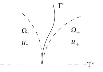
Starting from the blowup point $(1,0)$ of (1.1), let the formed shock curve $\Gamma$ be denoted by $x=\varphi(t)$ if the shock really appears. On the left hand side and right hand side of $\Gamma$ for $t\geq 1$ , the weak entropy solution $u$ is represented by $u_{-}$ and $u_{+}$ respectively (see Figure 1 below).

Refer to caption — Figure 1: Shock formation

It follows from the Rankine-Hugoniot condition and entropy condition on $\Gamma$ that

\displaystyle\varphi^{\prime}(t)[u](t,\varphi(t))=[f(u)](t,\varphi(t)),

(1.10)

where $[u](t,\varphi(t))=u_{+}(t,\varphi(t))-u_{-}(t,\varphi(t))$ is the jump of $u$ across $\Gamma$ , and

\displaystyle f^{\prime}(u_{+}(t,\varphi(t)))<\varphi^{\prime}(t)<f^{\prime}(u_{-}(t,\varphi(t))).

(1.11)

Our main results are

Theorem 1.1.

Under assumption (1.7), there exists a unique solution $u\in C^{1}((0,1)\times{\mathbb{R}})\cap C([0,1]\times{\mathbb{R}})$ to problem (1.1) together with (1.10)-(1.11) for $t\geq 1$ . Furthermore,

(1) $\varphi(t)\in C^{\frac{k+1}{k}}[1,1+\varepsilon)$ and $u\in C^{1}((1,1+\varepsilon)\times{\mathbb{R}})\setminus\{x=\varphi(t)\})$ for some $\varepsilon>0$ .

(2) near the blowup point $(1,0)$ , the behaviors of $u$ and its derivatives are as follows

$\displaystyle\|u(t,x)-u(1,0)\|$	$\displaystyle=$	$\displaystyle O(\|t-1\|^{\frac{1}{2k}}+\|x\|^{\frac{1}{2k+1}}),$	(1.12)
$\displaystyle\|\partial_{t}u(t,x)\|$	$\displaystyle=$	$\displaystyle O((\|t-1\|^{\frac{1}{2k}}+\|x\|^{\frac{1}{2k+1}})^{-(2k-1)}),$	(1.13)
$\displaystyle\|\partial_{x}u(t,x)\|$	$\displaystyle=$	$\displaystyle O((\|t-1\|^{\frac{1}{2k}}+\|x\|^{\frac{1}{2k+1}})^{-2k}).$	(1.14)

Theorem 1.2.

Under assumption (1.8), there exists a unique solution $u\in C^{1}((0,1)\times{\mathbb{R}})\cap C([0,1]\times{\mathbb{R}})$ to problem (1.1) together with (1.10)-(1.11) for $t\geq 1$ . Furthermore,

(i) $\varphi(t)\in C^{1}[1,1+\varepsilon]$ and $u\in C^{1}(((1,1+\varepsilon)\times{\mathbb{R}})\setminus\{x=\varphi(t)\})$ for some $\varepsilon>0$ . In addition, $\varphi(t)=O((t-1)|\ln(t-1)|^{-\frac{2}{p}})$ near $t=1$ and for $t>1$ .

(ii) near the blowup point $(1,0)$ , the behaviors of $u$ and its derivatives are as follows

$\displaystyle\|u(t,x)-u(1,0)\|$	$\displaystyle=$	$\displaystyle O(\|\ln\|t-1\|\|^{-\frac{1}{p}}+\|\ln\|x\|\|^{-\frac{1}{p}}),$	(1.15)
$\displaystyle\|\partial_{t}u(t,x)\|$	$\displaystyle=$	$\displaystyle O(\|t-1\|^{-1}\|\ln\|t-1\|\|^{-1-\frac{1}{p}}+\|x\|^{-1}\|\ln\|x\|\|^{-1-\frac{1}{p}}),$	(1.16)
$\displaystyle\|\partial_{x}u(t,x)\|$	$\displaystyle=$	$\displaystyle O(\|t-1\|^{-1}\|\ln\|t-1\|\|^{-1}+\|x\|^{-1}\|\ln\|x\|\|^{-1}).$	(1.17)

Remark 1.1.

If we take $k=1$ , then Theorem 1.1 coincides with the result in Theorem 2 of [11]. In addition, the author in [11] only shows the behaviors of $u$ in some part of the neighbourhood of the blowup point $(1,0)$ , which corresponds to the smallness of the variable $|\lambda|=\frac{|x|}{(t-1)^{\frac{3}{2}}}$ for $t>1$ . This can be referred to the proof of Lemma 2.1 in [11], where $|\lambda|$ is required to be small.

Remark 1.2.

The regularities of $\varphi(t)$ in Theorem 1.1 and Theorem 1.2 are optimal. One can see Remark 3.1 and Remark 4.1 below.

Remark 1.3.

Under the generic nondegenerate assumption of the initial data, for the 1-D $2\times 2$ $p-$ system of polytropic gases, the authors in [10]-[11] and [5] obtain the formation and construction of the shock wave starting from the blowup point under some variant conditions; for the 1-D $3\times 3$ strictly hyperbolic conservation laws with the small initial data or the 3-D full compressible Euler equations with symmetric structure and small perturbation, the authors in [4], [16] and [7] also get the formation and construction of the resulting shock waves, respectively.

In order to prove Theorem 1.1-1.2, our focus is to solve the singular and nonlinear ordinary differential equation (1.10) as in [11]. Note that the equation (1.10) is equivalent to $\varphi^{\prime}(t)=G(t,\varphi(t))\triangleq\int_{0}^{1}f^{\prime}(\theta u_{+}(t,\varphi(t))+(1-\theta)u_{-}(t,\varphi(t)))d\theta$ , where the function $G(t,\varphi)$ is not Lipschtzian with respect to variable $\varphi$ since the first order derivative of $u_{\pm}(t,x)$ with respect to the variable $x$ admits the strong singularities (see (1.13) and (1.17)). To get the uniqueness and regularity of $(\varphi(t),u_{\pm}(t,x))$ , we require to carefully analyze the behavior and regularity of solution $u$ near the blowup point $(1,0)$ . Due to the more degenerate conditions (1.5) and (1.6), we shall introduce some different transformations of $(t,x)$ from that in [11] (for examples, see (2.9), (2.20), (2.36) and so on). By involved computation, the behaviors of solution $u$ around the point $(1,0)$ are derived and then the optimal regularities of $\varphi(t)$ are also established. From our results, we have known two basic facts for problem (1.1): (1) Around the blowup point, the shock really appears whether the initial data are degenerate with finite orders or with infinite orders. (2) The optimal regularities of the shock solution and the resulting shock curve have explicit relations with the degenerate degrees of the initial data.

Our paper is organized as follows. In Section 2, we give some basic analysis on the characteristics envelope of equation (1.1) near $(1,0)$ , meanwhile, the detailed behaviors of the characteristics near $(1,0)$ are established. The proofs of Theorem 1.1 and Theorem 1.2 are given in Section 3 and Section 4 respectively.

2 Some preliminary

For problem (1.1), we define the characteristics $x=x(t,y)$ starting from the point $(0,y)$ as follows

\linespread{1.2}\begin{cases}&\displaystyle\frac{dx(t,y)}{dt}=f^{\prime}(u(t,x(t,y))),\\ &x(0,y)=y.\end{cases}

(2.1)

Then along this characteristics we have

u(t,x(t,y))\equiv u_{0}(y).

(2.2)

This means that the characteristics $x(t,y)$ is straight and

x(t,y)=y+tg(y).

(2.3)

For any fixed $t>0$ , in order to solve $y=y(t,x)$ in (2.3) such that the solution $u$ in (2.2) can be obtained, it is necessary to let

\frac{\partial x}{\partial y}(t,y)=1+tg^{\prime}(y)>0.

By assumption (1.7) or (1.8), we have that near $x=0$ ,

(i) for $0\leq t<1$ , $\frac{\partial x}{\partial y}(t,y)>0$ ;

(ii) $\frac{\partial x}{\partial y}(1,y)\geq 0$ , and only at $y=0$ , $\frac{\partial x}{\partial y}(1,y)=0$ .

Thus for $0\leq t\leq 1$ , one can get a function $y=y(t,x)$ satisfying (2.3) such that the solution to (1.1) is

u(t,x)=u_{0}(y(t,x)).

(2.4)

On the other hand, one can compute that for $0\leq t<1$ ,

\left\{\begin{array}[]{l}\frac{\partial y}{\partial t}=-\frac{g(y)}{1+tg^{\prime}(y)},\\ \frac{\partial y}{\partial x}=\frac{1}{1+tg^{\prime}(y)}.\end{array}\right.

(2.5)

This means that as $(t,x)$ tends to $(1-,0)$ , then $y(t,x)\rightarrow 0$ and $|\partial_{x}y(t,x)|\rightarrow+\infty$ .

Let $\varepsilon>0$ be a sufficiently small constant. Under assumption (1.2), it is easy to check that for $1<t<1+\varepsilon$ and $y$ near $0$ , there exist two roots of $\partial_{y}x(t,y)=0$ with respect to the variable $y$ , which are denoted by $\eta_{-}(t)$ and $\eta_{+}(t)$ with $\eta_{-}(t)<\eta_{+}(t)$ . Set $x_{\pm}(t)=x(t,\eta_{\pm}(t))$ , we then have

•

for $x<x_{+}(t)$ ( $x>x_{-}(t)$ resp.) and equality (2.3), there exists a unique root denoted by $y_{-}(t,x)$ ( $y_{+}(t,x)$ resp.).
•

for $x=x_{+}(t)$ ( $x=x_{-}(t)$ resp.) and equality (2.3), there exist two roots denoted by $y_{-}(t,x)<\eta_{+}(t)$ ( $\eta_{-}(t)<y_{+}(t,x)$ resp.).
•

for $x_{+}(t)<x<x_{-}(t)$ and equality (2.3), there exist three roots denoted by $y_{-}(t,x)<y_{0}(t,x)<y_{+}(t,x)$ .

Set

$\displaystyle\Omega_{-}$	$\displaystyle=$	$\displaystyle\{(t,x):1<t<1+\varepsilon,\ x<x_{-}(t)\}$
$\displaystyle\Omega_{+}$	$\displaystyle=$	$\displaystyle\{(t,x):1<t<1+\varepsilon,\ x>x_{+}(t)\}$
$\displaystyle\Omega_{0}$	$\displaystyle=$	$\displaystyle\{(t,x):1<t<1+\varepsilon,\ x_{+}(t)<x<x_{-}(t)\}.$

Under (1.7), we derive some properties of $\eta_{\pm}(t)$ and $x_{\pm}(t)$ near the blowup point $(1,0)$ .

Lemma 2.1.

There exists an $\varepsilon>0$ sufficiently small such that
(1) $\eta_{\pm}(t)\in C^{2k+1}(1,1+\varepsilon)\cap C^{\frac{1}{2k}}[1,1+\varepsilon)$ admit the following expansion

\eta_{\pm}(t)=\pm(2k+1)^{-\frac{1}{2k}}(t-1)^{\frac{1}{2k}}-\frac{g^{(2k+2)}(0)}{2k(2k)!}(2k+1)^{-\frac{2k+1}{k}}(t-1)^{\frac{1}{k}}+o((t-1)^{\frac{1}{k}});

(2.6)

(2) $x_{\pm}(t)=x(t,\eta_{\pm}(t))\in C^{2k+1}(1,1+\varepsilon)\cap C^{\frac{2k+1}{2k}}[1,1+\varepsilon)$ are the envelopes of the characteristic lines (2.3) which form a cusp at $(1,0)$ , meanwhile,

x_{\pm}(t)=\mp 2k(2k+1)^{-\frac{2k+1}{2k}}(t-1)^{\frac{2k+1}{2k}}+\frac{g^{(2k+2)}(0)}{(2k+2)!}(2k+1)^{-\frac{k+1}{k}}(t-1)^{\frac{k+1}{k}}+o((t-1)^{\frac{k+1}{k}}).

(2.7)

Proof.

(1) Note that $\eta_{\pm}(t)$ are the solutions of

1+tg^{\prime}(y)=-(t-1)+(2k+1)ty^{2k}+tr^{\prime}(y)=0.

(2.8)

This immediately yields $\eta_{\pm}\in C^{2k+1}(1,1+\varepsilon]$ by the implicit function theorem. For $t\to 1+$ , set

s=(t-1)^{\frac{1}{2k}},\ z=\frac{y}{s}.

(2.9)

Then (2.8) becomes

F(s,z)\triangleq(1+s^{2k})[(2k+1)z^{2k}+s^{-2k}r^{\prime}(sz)]-1=0.

(2.10)

Since $r^{\prime}(sz)=O(s^{2k+1})$ for $s$ near $0$ , $F(0,z^{0}_{\pm})=0$ holds for $z^{0}_{\pm}=\pm(2k+1)^{-\frac{1}{2k}}$ . By direct computation, we have that

	$\displaystyle\partial_{s}F(s,z)$	$\displaystyle=$	$\displaystyle 2k(2k+1)s^{2k-1}z^{2k}-2ks^{-2k-1}r^{\prime}(sz)+(s^{-2k}+1)zr^{\prime\prime}(sz),$		(2.11)
	$\displaystyle\partial_{z}F(s,z)$	$\displaystyle=$	$\displaystyle(1+s^{2k})[2k(2k+1)z^{2k-1}+s^{-2k+1}r^{\prime\prime}(sz)].$		(2.12)

Together with $r(sz)=\frac{g^{(2k+2)}(0)}{(2k+2)!}(sz)^{2k+2}+o(s^{2k+2})$ , this yields

	$\displaystyle\partial_{s}F(0,z^{0}_{\pm})$	$\displaystyle=$	$\displaystyle\pm\frac{g^{(2k+2)}(0)}{(2k+1)!}(2k+1)^{-\frac{2k+1}{2k}},$		(2.13)
	$\displaystyle\partial_{z}F(0,z^{0}_{\pm})$	$\displaystyle=$	$\displaystyle\pm 2k(2k+1)^{\frac{1}{2k}}\neq 0.$		(2.14)

By the implicit function theorem, for small $\varepsilon>0$ there exist

z=z_{\pm}(s)\in C^{2k+1}[0,\varepsilon]

(2.15)

such that $F(s,z_{\pm}(s))=0$ and

z_{\pm}(s)=z^{0}_{\pm}-\frac{g^{(2k+2)}(0)}{2k(2k)!}(2k+1)^{-\frac{2k+1}{k}}s+o(s).

(2.16)

Therefore, (2.6) is shown and then $\eta_{\pm}(t)\in C^{\frac{1}{2k}}[1,1+\varepsilon]$ .

(2) By (1.7) and (2.3), we have

x_{\pm}(t)=x(t,\eta_{\pm}(t))=-(t-1)\eta_{\pm}(t)+t\eta^{2k+1}_{\pm}(t)+tr(\eta_{\pm}(t)).

Together with (2.6), this yields $x_{\pm}(t)\in C^{2k+1}(1,1+\varepsilon]\cap C^{\frac{2k+1}{2k}}[1,1+\varepsilon]$ and the expansion (2.7). In addition, due to $\frac{\partial}{\partial y}x(t,\eta_{\pm}(t))=0$ , then for $t\in[1,1+\varepsilon]$ ,

\frac{d}{dt}x_{\pm}(t)=\frac{\partial}{\partial t}x(t,\eta_{\pm}(t))=g(\eta_{\pm}(t)).

(2.17)

This means that the tangent direction of $x=x_{\pm}(t)$ coincides with the characteristic speed of (2.3) at $(t,x_{\pm}(t))$ . Consequently, the proof of (2) is finished. ∎

Under (1.8)-(1.9), we have

Lemma 2.2.

For $\eta_{\pm}(t),\ x_{\pm}(t),\ y_{\pm}(t,x)$ and $y_{0}(t,x)$ , we can deduce the following properties for small $\varepsilon>0$ :
(1) $\eta_{\pm}(t)\in C^{\infty}(1,1+\varepsilon]\cap C[1,1+\varepsilon]$ with $\eta_{\pm}(\tau)=\pm|\ln(t-1)|^{-\frac{1}{p}}+O(\frac{\ln|\ln(t-1))|}{|\ln(t-1)|})$ .
(2) $x_{\pm}(t)=x(t,\eta_{\pm}(t))\in C^{\infty}(1,1+\varepsilon]\cap C^{1}[1,1+\varepsilon]$ are the envelopes of the characteristic lines and form a cusp at $(1,0)$ . Moreover we have the expansion $x_{\pm}(t)=\mp(t-1)|\ln(t-1)|^{-\frac{1}{p}}+O(\frac{(t-1)\ln|\ln(t-1)|}{|\ln(t-1)|})$ .
(3) For any $t\in(1,1+\varepsilon]$ , $y_{-}(t,\cdot)$ is an increasing function from $(-\infty,x_{-}(t)]$ onto $(-\infty,\eta_{-}(t)]$ ; $y_{0}(t,\cdot)$ is a decreasing function from $[x_{+}(t),x_{-}(t)]$ onto $[\eta_{-}(t),\eta_{+}(t)]$ ; $y_{+}(t,\cdot)$ is an increasing function from $[x_{+}(t),+\infty)$ onto $[\eta_{+}(t),+\infty)$ . Moreover, $y_{m}(t,x)\in C^{\infty}(\Omega_{m})\cap C(\bar{\Omega}_{m})$ , where $m=-,+,0$ .

Proof.

(1) Set $\tau=t-1$ for $t\geq 1$ . Note that $\eta_{\pm}(t)$ are defined for small $\tau>0$ and are the solutions of the following equation

1+tg^{\prime}(y)=\left(-\tau+\frac{1}{|y|^{p}}e^{-|y|^{-p}}\right)+\frac{\tau}{|y|^{p}}e^{-|y|^{-p}}+(\tau+1)e^{-|y|^{-p}}r_{1}(y)=0,

(2.18)

where $r_{1}(y)=\frac{1}{p}+\frac{yr_{0}(y)}{|y|^{p+2}}+r_{0}^{\prime}(y)=O(|y|^{\min\{-p+1,0\}})$ . Denote $\omega=|\ln\tau|^{-1}$ and $z=|y|^{-p}-(\omega^{-1}-\ln\omega)$ , then (2.18) becomes

F(\tau,z)\triangleq-1+\left(1+\omega z-\omega\ln\omega\right)e^{-z}+\omega e^{-z}\left(\tau\left(z+\omega^{-1}-\ln\omega\right)+(\tau+1)r_{1}(y)\right)=0.

(2.19)

Obviously, $F(0,0)=0$ . In addition, by direct computation, we have that for small $|y|$ ,

r^{\prime}_{1}(y)=-\frac{p+1}{|y|^{p+2}}r_{0}(y)+\frac{yr^{\prime}_{0}(y)}{|y|^{p+2}}+r^{\prime\prime}_{0}(y)=O(|y|^{-p})

and

\frac{\partial y}{\partial z}=-\frac{y|y|^{p}}{p}.

Thus one can check that

\frac{\partial F}{\partial z}=\omega e^{-z}-\left(1+z\omega-\omega\ln\omega\right)e^{-z}-\omega e^{-z}\left(\tau\left(z+\omega^{-1}-\ln\omega-1\right)+(\tau+1)(r_{1}(y)-r^{\prime}_{1}(y)\frac{\partial y}{\partial z})\right).

This yields $\frac{\partial F}{\partial z}(0,0)=-1$ by $|y|\lesssim\omega^{\frac{1}{p}}$ . Since $F(\tau,z)$ is continuous and has the continuous partial derivative $\frac{\partial F}{\partial z}$ near $(0,0)$ , it follows from the implicit function theorem that there exists a continuous function $z=z(\tau)$ near $z=0$ to satisfy $F(\tau,z)=0$ . This deduces $\eta_{\pm}(t)=\pm(|\ln\tau|+\ln|\ln\tau|+z(\tau))^{-\frac{1}{p}}=\pm|\ln\tau|^{-\frac{1}{p}}+O(\frac{\ln|\ln\tau|}{|\ln\tau|})$ . On the other hand, for $\tau>0$ , we have $\frac{\partial x}{\partial y}(t,y)\neq 0$ and $g^{\prime}\in C^{\infty}$ . Then by the implicit function theorem, $\eta_{\pm}(t)\in C^{\infty}(1,1+\varepsilon]$ hold.

(2) By (1.8) and (2.3), we have that for small $\tau>0$ ,

x_{\pm}(t)=-\tau\eta_{\pm}(t)+t(\frac{\eta_{\pm}(t)}{p}e^{-|\eta_{\pm}(t)|^{-p}}+r_{0}(\eta_{\pm}(t)))=\tau[-\eta_{\pm}(t)+t(\frac{\eta_{\pm}(t)}{p}+o(\eta_{\pm}(t)))e^{-|O(\frac{\ln|\ln\tau|}{|\ln\tau|})|}],

which derives $x_{\pm}(t)\in C^{\infty}(1,1+\varepsilon]\cap C[1,1+\varepsilon]$ . On the other hand, it holds that for $t\in(1,1+\varepsilon]$ ,

	$\displaystyle\frac{d}{dt}x_{\pm}(t)$	$\displaystyle=$	$\displaystyle\frac{\partial}{\partial t}x(t,\eta_{\pm}(t))+\frac{\partial}{\partial y}x(t,\eta_{\pm}(t))\frac{d}{dt}\eta_{\pm}(t)$
		$\displaystyle=$	$\displaystyle g(\eta_{\pm}(t)),$

which means that the tangent direction of $x=x_{\pm}(t)$ is same as the characteristic speed of (2.3) at $(t,x_{\pm}(t))$ . In addition, at the point $(1,0)$ , one has

$\displaystyle x^{\prime}_{\pm}(1)$	$\displaystyle=$	$\displaystyle\lim_{t\rightarrow 1_{+}}\frac{x_{\pm}(t,\eta_{\pm}(t))-0}{t-1}$
	$\displaystyle=$	$\displaystyle\lim_{t\rightarrow 1_{+}}[-\eta_{\pm}(t)+t(\frac{\eta_{\pm}(t)}{p}+o(\eta_{\pm}(t)))e^{O(\frac{\ln\|\ln\tau\|}{\|\ln\tau\|})}]$
	$\displaystyle=$	$\displaystyle 0$
	$\displaystyle=$	$\displaystyle g(0).$

Hence we finish the proof of (2).

(3) For any fixed $t\in(1,1+\varepsilon]$ , due to

\frac{\partial}{\partial y}x(t,y)\left\{\begin{array}[]{ll}>0,&\text{ for }y\in(-\infty,\eta_{-}(t))\cup(\eta_{+}(t),+\infty),\\ =0,&\text{ for }y=\eta_{\pm}(t),\\ <0,&\text{ for }y\in(\eta_{-}(t),\eta_{+}(t)),\end{array}\right.

then by the inverse function theorem, $y_{m}(t,\cdot)$ with $m=-,+,0$ are well defined and satisfy the corresponding monotonicity. Moreover, $y_{+}(t,\cdot)\in C^{\infty}(x_{+}(t),+\infty)\cap C[x_{+}(t),+\infty)$ , $y_{0}(t,\cdot)\in C^{\infty}(x_{+}(t),x_{-}(t))\cap C[x_{+}(t),x_{-}(t)]$ and $y_{-}(t,\cdot)\in C^{\infty}(-\infty,x_{-}(t))\cap C(-\infty,x_{-}(t)]$ .

On the other hand, because of $\partial_{y}x(t,x)\neq 0$ for $(t,x)\notin\{x=x_{\pm}(t)\}$ , thus it follows from the implicit function theorem that $y_{m}(t,x)\in C^{\infty}(\Omega_{m})$ , $m=-,+,0$ . For the continuity of $y_{m}(t,x)$ in $\bar{\Omega}_{m}$ , we take $y_{+}(t,x)$ as an example. By $x_{+}(t)\in C^{1}([1,1+\varepsilon])$ , we then get

|y_{+}(\bar{t},x_{+}(\bar{t}))-y_{+}(t,x)|=|y_{+}(\bar{t},x_{+}(\bar{t}))-y_{+}(t,x_{+}(t))|+|y_{+}(t,x_{+}(t))-y_{+}(t,x)|\rightarrow 0

as $(t,x)\rightarrow(\bar{t},x_{+}(\bar{t}))$ for $\bar{t}\in[1,1+\varepsilon]$ and $(t,x)\in\Omega_{+}$ . Thus $y_{+}(t,x)\in C^{\infty}(\Omega_{+})\cap C(\bar{\Omega}_{+})$ holds.
∎

To study the formation of shock wave and the regularity of the resulting shock $x=\varphi(t)$ to equation (1.1), it is required to study the properties of $y_{\pm}(t,x)$ for $(t,x)$ in the cusp domain $\Omega_{0}$ . Under assumption (1.5), motivated by [11], we take the following change of the variables

\tau=t-1,\ s=\tau^{\frac{1}{2k}},\ \mu=\frac{y}{s},\ \lambda=\frac{x}{s^{2k+1}},

(2.20)

and will establish the behavior of $y_{\pm}(t,x)$ near $(1,0)$ in some sub-domain of $\Omega_{0}$ .

Lemma 2.3.

For small $\varepsilon>0$ , under assumption (1.7), there exists some constant $\delta>0$ such that for $(s,\lambda)\in\{0\leq s\leq\varepsilon,\ |\lambda|\leq\delta\}$ , $(s,\lambda)\rightarrow s^{j}y_{\pm}(t,x)$ are of $C^{j+2}$ for $j=-1,0,1,\ldots,2k$ and $y_{\pm}(t,x)$ admit the following expansions

	$\displaystyle y_{+}(t,x)$	$\displaystyle=$	$\displaystyle s(1+\frac{\lambda}{2k}-\frac{g^{(2k+2)}(0)}{2k(2k+2)!}s)+O(s^{3}+s\lambda^{2}),$		(2.21)
	$\displaystyle y_{-}(t,x)$	$\displaystyle=$	$\displaystyle s(-1+\frac{\lambda}{2k}-\frac{g^{(2k+2)}(0)}{2k(2k+2)!}s)+O(s^{3}+s\lambda^{2}).$		(2.22)

Proof.

Let

h(y)\triangleq\frac{r(y)}{y^{2k+1}}=\int_{0}^{1}\frac{(1-\theta)^{2k}}{(2k)!}g^{(2k+1)}(\theta y)d\theta-1.

(2.23)

Then $h(y)\in C^{p-2k-1}$ and $h(0)=0$ . Furthermore,

yh^{\prime}(y)=\frac{y}{(2k)!}\int_{0}^{1}(1-\theta)^{2k}\theta g^{(2k+2)}(\theta y)d\theta=-\frac{1}{(2k)!}\int_{0}^{1}g^{(2k+1)}(\theta y)(1-\theta)^{2k-1}[1-(2k+1)\theta]~{}d\theta.

(2.24)

This derives $yh^{\prime}(y)\in C^{1}$ . Similarly, $y^{j}h^{(j)}(y)\in C^{1}$ holds for $j=2,\ldots,2k+1$ . Divided by $s^{2k}$ , (2.3) becomes

G(s,\lambda,\mu)\triangleq-\mu+(1+s^{2k})\mu^{2k+1}+(1+s^{2k})\mu^{2k+1}h(s\mu)-\lambda=0.

(2.25)

For $s=\lambda=0$ , by $G(0,0,\mu)=-\mu+\mu^{2k+1}=-\mu(1-\mu^{2k})=0$ we get the roots $\mu^{0}_{\pm}=\pm 1$ and $\mu^{0}_{c}=0$ . Note that

\partial_{\mu}G(s,\lambda,\mu)=-1+(2k+1)(1+s^{2k})\mu^{2k}+(1+s^{2k})((2k+1)\mu^{2k}h(s\mu)+\mu^{2k+1}sh^{\prime}(s\mu)).

(2.26)

Then

\partial_{\mu}G(0,0,\pm 1)=2k\neq 0.

(2.27)

By the implicit function theorem, there exist functions $\mu=\mu_{\pm}(s,\lambda)\in C^{1}$ near $(s,\lambda)=(0,0)$ such that

G(s,\lambda,\mu_{\pm}(s,\lambda))=0,\ \mu_{\pm}(0,0)=\pm 1,

(2.28)

and then $s^{-1}y_{\pm}\in C^{1}$ . On the other hand, due to

	$\displaystyle\partial_{s}G(s,\lambda,\mu)$	$\displaystyle=$	$\displaystyle 2ks^{2k-1}\mu^{2k}+2ks^{2k-1}\mu^{2k+1}h(s\mu)+(1+s^{2k})\mu^{2k+2}h^{\prime}(s\mu),$		(2.29)
	$\displaystyle\partial_{\lambda}G(s,\lambda,\mu)$	$\displaystyle=$	$\displaystyle-1,$		(2.30)

then

	$\displaystyle\partial_{s}G(0,0,\pm 1)$	$\displaystyle=$	$\displaystyle h^{\prime}(0)=\frac{g^{(2k+2)}(0)}{(2k)!}\int_{0}^{1}(1-\theta)^{2k}\theta d\theta=\frac{g^{(2k+2)}(0)}{(2k+2)!}$		(2.31)
	$\displaystyle\partial_{\lambda}G(0,0,\pm 1)$	$\displaystyle=$	$\displaystyle-1.$		(2.32)

It follows from (2.27), (2.31) and (2.32) that

\partial_{s}\mu_{\pm}(0,0)=-\frac{g^{(2k+2)}(0)}{2k(2k+2)!},\quad\partial_{\lambda}\mu_{\pm}(0,0)=\frac{1}{2k}.

(2.33)

Consequently, the expansions (2.21) and (2.22) are shown.

We next prove $(s,\lambda)\rightarrow y_{\pm}\in C^{2}$ . By

s\partial_{s}G(s,\lambda,\mu_{\pm})+\partial_{\mu}G(s,\lambda,\mu_{\pm})(s\partial_{s}\mu_{\pm}(s,\lambda))=0

(2.34)

and

s\partial_{s}G(s,\lambda,\mu_{\pm}(s,\lambda))=2ks^{2k}\mu_{\pm}^{2k}+2ks^{2k}\mu_{\pm}^{2k+1}h(s\mu_{\pm})+(1+s^{2k})\mu_{\pm}^{2k+1}(s\mu_{\pm}h^{\prime}(s\mu_{\pm}))\in C^{1},

(2.35)

we then have $s\partial_{s}\mu_{\pm}(s,\lambda)\in C^{1}$ . Thus from $\partial_{s}y_{\pm}=\mu_{\pm}+s\partial_{s}\mu_{\pm}$ , one can see that $(s,\lambda)\to y_{\pm}$ is of $C^{1}$ . In addition, by $\partial_{\lambda}y_{\pm}=s\partial_{\lambda}\mu_{\pm}(s,\lambda)$ and similar computation, we can get $y_{\pm}\in C^{2}$ with respect to $s$ and $\lambda$ .

Note that

	$\displaystyle s^{j}\partial^{j}_{s}G(s,\lambda,\mu_{\pm}(s,\lambda))$	$\displaystyle=$	$\displaystyle{\mathcal{G}}(s,\lambda,s\partial_{s}\mu_{\pm},\ldots,s^{j-1}\partial^{j-1}_{s}\mu_{\pm},h(s\mu_{\pm}),(s\mu_{\pm})h^{\prime}(s\mu_{\pm}),\ldots,(s\mu_{\pm})^{j}h^{(j)}(s\mu_{\pm}))$
			$\displaystyle+\partial_{\mu}G(s,\lambda,\mu_{\pm})(s^{j}\partial^{j}_{s}\mu_{\pm}(s,\lambda)),\ j=2,3,\ldots,2k+1,$

where ${\mathcal{G}}$ is a polynomial with respect to its arguments. Then $s^{j}\partial^{j}_{s}\mu_{\pm}(s,\lambda)\in C^{1}$ for $j=2,3,\ldots,2k+1$ by induction. Similarly, $s^{j}\partial^{m}_{\lambda}\partial^{j-m}_{s}\mu_{\pm}(s,\lambda)\in C^{1}$ for $1\leq m\leq j\leq 2k+1$ . Consequently, the proof of $(s,\lambda)\rightarrow s^{j}y_{\pm}(t,x)\in C^{j+2}$ for $j=-1,0,1,\ldots,2k$ is completed. ∎

Under assumption (1.8), we now study the asymptotic behavior of $y_{\pm}(t,x)$ near $(1,0)$ . In this case, we take the following change of the variables

\tau=t-1,\ s=|\ln\tau|^{-\frac{1}{p}},\ \lambda=\frac{x}{s\tau},\ \mu=\frac{y}{s}.

(2.36)

Then we obtain

Lemma 2.4.

Under assumption (1.8), there exist some small constants $\varepsilon$ , $\delta>0$ such that for $(t,x)\in\Omega_{0}\triangleq\{1\leq t\leq 1+\varepsilon,\ -\delta s\tau<x<\delta s\tau\}$ , $y_{\pm}\in C^{1+p}$ hold for the variables $s$ and $\lambda$ . Furthermore,

	$\displaystyle y_{+}(t,x)$	$\displaystyle=$	$\displaystyle s\left(1+\frac{\ln p}{p}s^{p}+\frac{s^{p}\lambda}{p}\right)+O\left(s^{\min\{p+2,2p+1\}}+s^{p+1}\|\lambda\|^{2}\right),$		(2.37)
	$\displaystyle y_{-}(t,x)$	$\displaystyle=$	$\displaystyle s\left(-1-\frac{\ln p}{p}s^{p}+\frac{s^{p}\lambda}{p}\right)+O\left(s^{\min\{p+2,2p+1\}}+s^{p+1}\|\lambda\|^{2}\right).$		(2.38)

Proof.

By divided by $s\tau$ , (2.3) can be written as follows

G(s,\lambda,\mu)\triangleq\mu(-1+\frac{1}{p}e^{s^{-p}(1-|\mu|^{-p})})+\frac{\mu}{p}e^{-s^{-p}|\mu|^{-p}}+\frac{e^{s^{-p}}+1}{s}e^{-s^{-p}|\mu|^{-p}}r_{0}(s\mu)-\lambda=0.

(2.39)

Below we assume $\mu\neq 0$ . Without loss of generality, one can assume $\mu>0$ (corresponding to the case of $y_{+}(t,x)$ ). We divide the proof of Lemma 2.4 into the two cases of $p\geq 1$ and $p\in(0,1)$ .

Case 1. $p\geq 1$ .

Set $\zeta=s^{-p}(1-\mu^{-p})-\ln p$ and $\mu=\left(1-s^{p}(\zeta+\ln p)\right)^{-\frac{1}{p}}$ . Then (2.39) becomes

F_{1}(s,\lambda,\zeta)\triangleq G(s,\lambda,\mu)=\mu(-1+e^{\zeta})+\mu e^{\zeta-s^{-p}}+\frac{pe^{\zeta}(1+e^{-s^{-p}})}{s}r_{0}(s\mu)-\lambda.

(2.40)

Obviously $F_{1}(0,0,0)=0$ and $\displaystyle\lim_{s\to 0+,\zeta\to 0}\mu=1$ . Note that

\partial_{s}\mu=s^{p-1}(\zeta+\ln p)\left(1-s^{p}(\zeta+\ln p)\right)^{-\frac{1}{p}-1},\quad\partial_{\zeta}\mu=\frac{s^{p}}{p}\left(1-s^{p}(\zeta+\ln p)\right)^{-\frac{1}{p}-1}.

Thanks to $p\geq 1$ , we have that $\partial_{s}\mu$ is bounded. On the other hand,

$\displaystyle\partial_{s}F_{1}$	$\displaystyle=$	$\displaystyle ps^{-p-1}\mu e^{\zeta-s^{-p}}+\left(-1+e^{\zeta}+e^{\zeta-s^{-p}}\right)\partial_{s}\mu$
		$\displaystyle+\frac{pe^{\zeta}\left(e^{-s^{-p}}(ps^{-p}-1)-1\right)}{s^{2}}r_{0}(s\mu)+\frac{pe^{\zeta}(1+e^{-s^{-p}})}{s}r^{\prime}_{0}(s\mu)\left(\mu+s\partial_{s}\mu\right),$
$\displaystyle\partial_{\lambda}F_{1}$	$\displaystyle=$	$\displaystyle-1,$
$\displaystyle\partial_{\zeta}F_{1}$	$\displaystyle=$	$\displaystyle\mu\left(e^{\zeta}+e^{\zeta-s^{-p}}\right)+\left(-1+e^{\zeta}+e^{\zeta-s^{-p}}\right)\partial_{\zeta}\mu+\frac{pe^{\zeta}(1+e^{-s^{-p}})}{s}\left(r_{0}(s\mu)+sr^{\prime}_{0}(s\mu)\partial_{\zeta}\mu\right).$

This derives $F_{1}\in C^{1}$ and

\partial_{s}F_{1}(0,0,0)=\frac{p}{2}r^{\prime\prime}_{0}(0),\quad\partial_{\lambda}F_{1}(0,0,0)=-1,\quad\partial_{\zeta}F_{1}(0,0,0)=1.

(2.41)

Thus by the implicit function theorem, one can obtain that there exists a unique function $\zeta(s,\lambda)\in C^{1}$ satisfying $F_{1}(s,\lambda,\zeta(s,\lambda))=0$ and admitting the following expansion

\zeta(s,\lambda)=\frac{p}{2}r^{\prime\prime}_{0}(0)s+\lambda+O\left(s^{2}+\lambda^{2}\right).

(2.42)

At this time, we get

$\displaystyle\mu(s,\lambda)$	$\displaystyle=$	$\displaystyle\left(1-s^{p}(\zeta+\ln p)\right)^{-\frac{1}{p}}$	(2.43)
	$\displaystyle=$	$\displaystyle\left(1-s^{p}(\ln p+\frac{p}{2}r^{\prime\prime}_{0}(0)s+\lambda+O\left(s^{2}+\lambda^{2}\right)\right)^{-\frac{1}{p}}$
	$\displaystyle=$	$\displaystyle 1+\frac{\ln p}{p}s^{p}+\frac{s^{p}\lambda}{p}+O\left(s^{p+1}+s^{p}\|\lambda\|^{2}\right)$

and $s^{l}\mu\in C^{l+p}$ , $l=0,1$ .

If we consider the case of $\mu<0$ , then by the same method, one can obtain the expansion

\mu(s,\lambda)=-1-\frac{\ln p}{p}s^{p}+\frac{s^{p}\lambda}{p}+O\left(s^{p+1}+s^{p}|\lambda|^{2}\right).

(2.44)

Case 2. $0<p<1$ .

Set $\omega=s^{p}$ , $\zeta=\omega^{-1}(1-\mu^{-p})-\ln p$ and $\mu=\left(1-\omega(\zeta+\ln p)\right)^{-\frac{1}{p}}$ . Then (2.39) becomes

F_{2}(\omega,\lambda,\zeta)\triangleq G(s,\lambda,\mu)=\mu(-1+e^{\zeta})+\mu e^{\zeta-\omega^{-1}}+\frac{pe^{\zeta}(1+e^{-\omega^{-1}})}{\omega^{\frac{1}{p}}}r_{0}(\omega^{\frac{1}{p}}\mu)-\lambda.

(2.45)

Obviously $F_{2}(0,0,0)=0$ and $\displaystyle\lim_{\omega\to 0+,\ \zeta\to 0}\mu=1$ . Note that

\partial_{\omega}\mu=\frac{\zeta+\ln p}{p}\left(1-\omega(\zeta+\ln p)\right)^{-\frac{1}{p}-1},\quad\partial_{\zeta}\mu=\frac{\omega}{p}\left(1-\omega(\zeta+\ln p)\right)^{-\frac{1}{p}-1}.

On the other hand,

$\displaystyle\partial_{\omega}F_{2}$	$\displaystyle=$	$\displaystyle\omega^{-2}\mu e^{\zeta-\omega^{-1}}+\left(-1+e^{\zeta}+e^{\zeta-\omega^{-1}}\right)\partial_{\omega}\mu$
		$\displaystyle+\frac{e^{\zeta}\left(e^{-\omega^{-1}}(p\omega^{-1}-1)-1\right)}{\omega^{\frac{1}{p}+1}}r_{0}(\omega^{\frac{1}{p}}\mu)+\frac{pe^{\zeta}(1+e^{-\omega^{-1}})}{\omega^{\frac{1}{p}}}r^{\prime}_{0}(\omega^{\frac{1}{p}}\mu)\cdot\omega^{\frac{1}{p}-1}\left(\frac{1}{p}\mu+\omega\partial_{\omega}\mu\right),$
$\displaystyle\partial_{\lambda}F_{2}$	$\displaystyle=$	$\displaystyle-1,$
$\displaystyle\partial_{\zeta}F_{2}$	$\displaystyle=$	$\displaystyle\mu\left(e^{\zeta}+e^{\zeta-\omega^{-1}}\right)+\left(-1+e^{\zeta}+e^{\zeta-\omega^{-1}}\right)\partial_{\zeta}\mu+\frac{pe^{\zeta}(1+e^{-\omega^{-1}})}{\omega^{\frac{1}{p}}}\left(r_{0}(\omega^{\frac{1}{p}}\mu)+\omega^{\frac{1}{p}}r^{\prime}_{0}(\omega^{\frac{1}{p}}\mu)\partial_{\zeta}\mu\right).$

Then $F_{2}\in C^{1}$ and

\partial_{\omega}F_{2}(0,0,0)=0,\quad\partial_{\lambda}F_{2}(0,0,0)=-1,\quad\partial_{\zeta}F_{2}(0,0,0)=1.

(2.46)

Thus by the implicit function theorem, one can obtain that there exists a unique function $\zeta(\omega,\lambda)\in C^{1}$ satisfying $F_{2}(\omega,\lambda,\zeta(\omega,\lambda))=0$ and admitting such an expansion

\zeta(\omega,\lambda)=\lambda+O\left(\omega^{2}+\lambda^{2}\right).

(2.47)

This yields

$\displaystyle\mu(s,\lambda)$	$\displaystyle=$	$\displaystyle\left(1-s^{p}\left(\zeta(s^{p},\lambda)+\ln p\right)\right)^{-\frac{1}{p}}$	(2.48)
	$\displaystyle=$	$\displaystyle\left(1-s^{p}(\ln p+\lambda+O\left(s^{2p}+\lambda^{2}\right)\right)^{-\frac{1}{p}}$
	$\displaystyle=$	$\displaystyle 1+\frac{\ln p}{p}s^{p}+\frac{s^{p}\lambda}{p}+O\left(s^{2p}+s^{p}\|\lambda\|^{2}\right)$

and $s^{l}\mu\in C^{l+p}$ for $l=0,1$ .

If we consider the case of $\mu<0$ , then by the same method, one can obtain the expansion

\mu(s,\lambda)=-1-\frac{\ln p}{p}s^{p}+\frac{s^{p}\lambda}{p}+O\left(s^{2p}+s^{p}|\lambda|^{2}\right).

(2.49)

Consequently, we complete the proof of (2.37) and (2.38).

∎

3 Proof of Theorem 1.1

We now construct the shock curve $x=\varphi(t)$ of (1.1) in $\Omega_{0}$ . It follows from the Rankine-Hugoniot condition that

\left\{\begin{array}[]{l}\varphi^{\prime}(t)=\frac{f(u_{0}(y_{+}(t,\varphi(t))))-f(u_{0}(y_{-}(t,\varphi(t))))}{u_{0}(y_{+}(t,\varphi(t)))-u_{0}(y_{-}(t,\varphi(t)))},\\ \varphi(1)=0.\end{array}\right.

(3.1)

This, together with the mean-value theorem, yields

g(y_{+}(t,\varphi(t)))<\varphi^{\prime}(t)<g(y_{-}(t,\varphi(t))),

(3.2)

which means that the entropy condition on $x=\varphi(t)$ holds. Denote

a(x,y)\triangleq\left\{\begin{array}[]{ll}\frac{f(u_{0}(x))-f(u_{0}(y))}{u_{0}(x)-u_{0}(y)},&\text{ if }x\neq y,\\ g(x),&\text{ if }x=y.\end{array}\right.

(3.3)

Under assumption (1.7), it is easy to verify $a(x,y)\in C^{2k+2}({\mathbb{R}}^{2})$ with $a(x,y)=-\frac{1}{2}(x+y)+b(x,y)$ , where $b(x,y)=O(x^{2}+y^{2})\in C^{2k+2}$ .

Lemma 3.1.

Under assumption (1.7), for (3.1) and small $\varepsilon>0$ , there exists a solution $x=\varphi(t)$ on $[1,1+\varepsilon)$ to satisfy
(1) $\varphi(t)$ is a $C^{2}$ function on $s\in[0,\varepsilon)$ , where $s=(t-1)^{\frac{1}{2k}}$ ;
(2) $\varphi(t)\in C^{\frac{k+1}{k}}[1,1+\varepsilon)$ .

Proof.

(1) Set $\lambda(s)=\frac{\varphi(t)}{s^{2k+1}}$ . Then (3.1) becomes

\left\{\begin{array}[]{l}s\lambda^{\prime}(s)+(2k+2)\lambda(s)=sd(s,\lambda(s)),\\ \lambda(0)=0,\end{array}\right.

(3.4)

where

d(s,\lambda)=-\frac{k(\mu_{+}(s,\lambda)+\mu_{-}(s,\lambda)-\lambda)}{s}+\frac{2k}{s^{2}}b(s\mu_{+}(s,\lambda),s\mu_{-}(s,\lambda)).

(3.5)

By the proof procedure of Lemma 2.3, we have $s^{j}d(s,\lambda)\in C^{j}$ for $j=0,1,2$ . Then by the same analysis in [11], there exists a unique solution $\lambda(s)\in C^{1}[0,\varepsilon)$ to (3.4) and further $s\lambda^{\prime}(s)\in C^{1}$ . Due to $(s\lambda(s))^{\prime}=s\lambda^{\prime}(s)+\lambda(s)$ , then $s\lambda(s)\in C^{2}$ , and $s^{2}\lambda^{\prime}(s)=s^{2}d-(2k+1)s\lambda\in C^{2}$ . Therefore, $s\rightarrow\varphi^{\prime}(t)=\frac{1}{2k}[s^{2}\lambda^{\prime}(s)+(2k+1)s\lambda(s)]$ is a $C^{2}$ function.

(2) Let $s\rightarrow 0+$ in (3.4), we have

\lambda^{\prime}(0)=\frac{d(0,0)}{2k+3}=\frac{g^{(2k+2)}(0)}{(2k+3)!}+\lim_{s\rightarrow 0_{+}}\frac{b(s\mu_{+},s\mu_{-})}{s^{2}}=O(1).

Therefore $\lambda(s)=O(s)$ and then $\varphi(t)=O(s^{2k+2})=O((t-1)^{\frac{k+1}{k}})\in C^{\frac{k+1}{k}}[1,1+\varepsilon)$ .

∎

Remark 3.1. The regularity of $\varphi(t)$ in Lemma 3.1 is optimal. Indeed, we consider the following problem

\left\{\begin{array}[]{ll}&\partial_{t}u+\partial_{x}(\frac{1}{2}u^{2})=0,\\ &\displaystyle u(0,x)=-x+x^{2k+1}+|x|^{2k+2+\varepsilon},\ \varepsilon>0.\end{array}\right.

In this case, we have $g(x)=-x+x^{2k+1}+x^{2k+2}$ and

	$\displaystyle y_{+}(t,\varphi(t))$	$\displaystyle=$	$\displaystyle(t-1)^{\frac{1}{2k}}(1+\frac{\varphi(t)}{2k(t-1)^{\frac{2k+1}{2k}}}-\frac{(t-1)^{\frac{1}{2k}}}{2k})+o((t-1)^{\frac{1}{k}})$
	$\displaystyle y_{-}(t,\varphi(t))$	$\displaystyle=$	$\displaystyle(t-1)^{\frac{1}{2k}}(-1+\frac{\varphi(t)}{2k(t-1)^{\frac{2k+1}{2k}}}-\frac{(t-1)^{\frac{1}{2k}}}{2k})+o((t-1)^{\frac{1}{k}}).$		(3.6)

It follows from Rankine-Hugoniot condition that

	$\displaystyle\varphi^{\prime}(t)$	$\displaystyle=$	$\displaystyle-\frac{y_{-}(t,\varphi(t))+y_{+}(t,\varphi(t))}{2}$
		$\displaystyle=$	$\displaystyle\frac{\varphi(t)}{k(t-1)}-\frac{(t-1)^{\frac{1}{k}}}{k}+o((t-1)^{\frac{1}{k}}).$

This derives $\varphi(t)\in C^{\frac{k+1}{k}}[1,1+\varepsilon)$ which is optimal.

Lemma 3.2.

Under assumption (1.7), for any $c\in(-\frac{2k}{(2k+1)^{\frac{1}{2k}+1}},+\infty)$ , there exist $\varepsilon=\varepsilon(c)>0$ and $\delta=\delta(c)>0$ such that for $(s,\lambda)\in\{0<s<\varepsilon,c-\delta<\lambda<c+\delta\}$ , $(s,\lambda)\rightarrow y_{+}(t,x)$ has the expansion

y_{+}(t,x)=s\left(\mu_{c}-\frac{\mu_{c}^{2k+2}g^{(2k+2)}(0)}{(-1+\mu_{c}^{2k})(2k+2)!}s+\frac{\lambda-c}{-1+\mu_{c}^{2k}}\right)+O(s^{3}+s(\lambda-c)^{2}),

(3.7)

and for $(s,\lambda)\in\{0<s<\varepsilon,-c-\delta<\lambda<-c+\delta\}$ , $(s,\lambda)\rightarrow y_{-}(t,x)$ has the expansion

y_{-}(t,x)=s\left(-\mu_{c}-\frac{\mu_{c}^{2k+2}g^{(2k+2)}(0)}{(-1+\mu_{c}^{2k})(2k+2)!}s+\frac{\lambda+c}{-1+\mu_{c}^{2k}}\right)+O(s^{3}+s(\lambda+c)^{2}),

(3.8)

where $\mu_{c}$ is the unique solution in $(\frac{1}{(2k+1)^{\frac{1}{2k}}},+\infty)$ of the equation

G(0,c,\mu)=-\mu+\mu^{2k+1}-c=0.

(3.9)

Proof.

By (2.26), (2.29) and (2.30), we have that

$\displaystyle\partial_{\mu}G(0,\pm c,\pm\mu_{c})$	$\displaystyle=$	$\displaystyle-1+(2k+1)\mu_{c}^{2k}>0,$	(3.10)
$\displaystyle\partial_{s}G(0,\pm c,\pm\mu_{c})$	$\displaystyle=$	$\displaystyle\mu_{c}^{2k+2}h^{\prime}(0)=\frac{\mu_{c}^{2k+2}g^{(2k+2)}(0)}{(2k+2)!},$	(3.11)
$\displaystyle\partial_{\lambda}G(0,\pm c,\pm\mu_{c})$	$\displaystyle=$	$\displaystyle-1.$	(3.12)

Then by the implicit function theorem one has that there is a unique function $\mu_{\pm}(s,\lambda)$ near $(0,\pm c)$ satisfying $G(s,\lambda,\mu_{\pm}(s,\lambda))\equiv 0$ and admitting the expansion

\mu_{\pm}(s,\lambda)=\pm\mu_{c}-\frac{1}{-1+\mu_{c}^{2k}}\left(\frac{\mu_{c}^{2k+2}g^{(2k+2)}(0)}{(2k+2)!}s-(\lambda-c)\right)+O(s^{2}+(\lambda-c)^{2}).

(3.13)

Thus (3.7) and (3.8) are proved. ∎

To study the asymptotic behavior of $y_{\pm}$ near the $x-$ axis, we now take the following transform

\xi=x^{\frac{1}{2k+1}},\ \eta=\frac{t-1}{\xi^{2k}},\ \nu=\frac{y}{\xi}.

(3.14)

Under assumption (1.6), by divided $\xi^{2k+1}$ , (2.3) then becomes

H(\eta,\xi,\nu)\triangleq-\eta\nu+(1+\xi^{2k}\eta)\nu^{2k+1}+(1+\xi^{2k}\eta)\nu^{2k+1}h(\xi\nu)-1=0.

(3.15)

We now have

Lemma 3.3.

Under assumption (1.6), for small $\delta>0$ , there exists some small constant $\varepsilon>0$ such that for $(\eta,\xi)\in\{|\eta|\leq\varepsilon,\ 0<\xi<\delta\}$ , we can get the expansion of $y_{+}(t,x)$ on $(\xi,\eta)$

y_{+}(t,x)=\xi\left(1+\frac{\eta}{2k+1}-\frac{g^{(2k+2)}(0)}{(2k+2)!}\xi\right)+O(\eta^{2}\xi+\xi^{3}),

(3.16)

and for $(\eta,\xi)\in\{|\eta|\leq\varepsilon,\ -\delta<\xi<0\}$ , we can get

y_{-}(t,x)=\xi\left(1-\frac{\eta}{2k+1}-\frac{g^{(2k+2)}(0)}{(2k+2)!}\xi\right)+O(\eta^{2}\xi+\xi^{3}).

(3.17)

Proof.

It follows from direct computation that $H(0,0,1)=0$ and

$\displaystyle\partial_{\nu}H$	$\displaystyle=$	$\displaystyle-\eta+(2k+1)(1+\xi^{2k}\eta)\nu^{2k}+(2k+1)(1+\xi^{2k}\eta)\nu^{2k}h(\xi\nu)+(1+\xi^{2k}\eta)\nu^{2k+1}\xi h^{\prime}(\xi\nu),$	(3.18)
$\displaystyle\partial_{\eta}H$	$\displaystyle=$	$\displaystyle-\nu+\xi^{2k}\nu^{2k+1}+\xi^{2k}\nu^{2k+1}h(\xi\nu),$	(3.19)
$\displaystyle\partial_{\xi}H$	$\displaystyle=$	$\displaystyle 2k\xi^{2k-1}\eta\nu^{2k+1}+2k\xi^{2k-1}\eta\nu^{2k+1}h(\xi\eta)+(1+\xi^{2k}\eta)\nu^{2k+1}\nu h^{\prime}(\xi\nu).$	(3.20)

Then

$\displaystyle\partial_{\nu}H(0,0,1)$	$\displaystyle=$	$\displaystyle 2k+1,$	(3.21)
$\displaystyle\partial_{\eta}H(0,0,1)$	$\displaystyle=$	$\displaystyle-1,$	(3.22)
$\displaystyle\partial_{\xi}H(0,0,1)$	$\displaystyle=$	$\displaystyle h^{\prime}(0)=\frac{g^{(2k+2)}(0)}{(2k+2)!}.$	(3.23)

By the implicit function theorem, there exists a unique solution $\nu=\nu(\eta,\xi)$ of (3.15) near $(\eta,\xi)=(0,0)$ such that

\nu(\eta,\xi)=1+\frac{\eta}{2k+1}-\frac{g^{(2k+2)}(0)}{(2k+2)!}\xi+O(\eta^{2}+\xi^{2}).

(3.24)

Therefore, we obtain (3.16) for $\xi>0$ . Analogously, (3.17) holds for $\xi<0$ . ∎

Next we consider the asymptotic behavior of $y(t,x)$ near the blowup point $(1,0)$ in the domain $\{(t,x):\ t<1\}$ . Without confusions, we still use the same notation as for $t>1$ . Note that through each point in $\{t<1\}$ , there exists a unique characteristic line. By taking the following transform similar to (2.20)

\tau=1-t,\ s=\tau^{\frac{1}{2k}},\ \mu=\frac{y}{s},\ \lambda=\frac{x}{s^{2k+1}},

(3.25)

and then by divided $s^{2k+1}$ on two sides of (2.3), then (2.3) becomes

G(s,\lambda,\mu)\triangleq\mu+(1-s^{2k})\mu^{2k+1}+(1-s^{2k})\mu^{2k+1}h(s\mu)-\lambda=0.

(3.26)

Lemma 3.4.

For each $c\in{\mathbb{R}}$ , there exist $\varepsilon=\varepsilon(c),\delta=\delta(c)>0$ such that for $(s,\lambda)\in\{0<s<\varepsilon,c-\delta<\lambda<c+\delta\}$ , $(s,\lambda)\rightarrow y(t,x)$ has the expansion

y(t,x)=s\left(\mu_{c}-\frac{\mu_{c}^{2k+2}g^{(2k+2)}(0)}{(1+(2k+1)\mu_{c}^{2k})(2k+2)!}s-\frac{\lambda-c}{1+(2k+1)\mu_{c}^{2k}}\right)+O(s^{3}+s(\lambda-c)^{2}),

(3.27)

where $\mu_{c}$ is the unique solution of the equation

G(0,c,\mu)=\mu+\mu^{2k+1}-c=0.

(3.28)

Proof.

It follows from direct computation that

$\displaystyle\partial_{\mu}G(s,\lambda,\mu)$	$\displaystyle=$	$\displaystyle 1+(2k+1)(1-s^{2k})\mu^{2k}+(2k+1)(1-s^{2k})\mu^{2k+1}sh^{\prime}(s\mu),$	(3.29)
$\displaystyle\partial_{s}G(s,\lambda,\mu)$	$\displaystyle=$	$\displaystyle-2ks^{2k-1}\mu^{2k+1}-2ks^{2k-1}\mu^{2k+1}h(s\mu)+(1-s^{2k})\mu^{2k+2}h^{\prime}(s\mu),$	(3.30)
$\displaystyle\partial_{\lambda}G(s,\lambda,\mu)$	$\displaystyle=$	$\displaystyle-1.$	(3.31)

Then

$\displaystyle\partial_{\mu}G(0,c,\mu_{c})$	$\displaystyle=$	$\displaystyle 1+(2k+1)\mu_{c}^{2k}>0,$	(3.32)
$\displaystyle\partial_{s}G(0,c,\mu_{c})$	$\displaystyle=$	$\displaystyle\mu_{c}^{2k+2}h^{\prime}(0)=\frac{\mu_{c}^{2k+2}g^{(2k+2)}(0)}{(2k+2)!},$	(3.33)
$\displaystyle\partial_{\lambda}G(0,c,\mu_{c})$	$\displaystyle=$	$\displaystyle-1.$	(3.34)

By the implicit function theorem, there exists a $\mu(s,\lambda)$ near $(c,\mu_{c})$ satisfying

\mu(s,\lambda)=\mu_{c}-\frac{1}{1+(2k+1)\mu_{c}^{2k}}\left(\frac{\mu_{c}^{2k+2}g^{(2k+2)}(0)}{(2k+2)!}s-(\lambda-c)\right)+O(s^{2}+(\lambda-c)^{2}),

(3.35)

from which we can deduce (3.27). ∎

We start to prove Theorem 1.1.

Proof of Theorem 1.1:

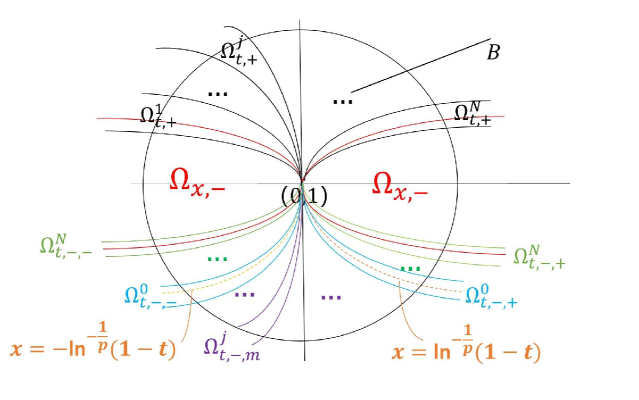
(1) By Lemma 3.1, $\varphi(t)\in C^{\frac{k+1}{k}}[1,1+\varepsilon)$ and $u\in C^{1}((1,1+\varepsilon)\times{\mathbb{R}})\setminus\{x=\varphi(t)\})$ for small $\varepsilon>0$ have been shown.

(2) Let $\delta,\ \varepsilon>0$ be the constants obtained in Lemma 3.3 and denote

$\displaystyle\Omega_{x,+}$	$\displaystyle=$	$\displaystyle B\cap\{(t,x):\ 0<x<\delta^{2k+1},\ \|t-1\|<\varepsilon x^{\frac{2k}{2k+1}}\},$	(3.36)
$\displaystyle\Omega_{x,-}$	$\displaystyle=$	$\displaystyle B\cap\{(t,x):\ -\delta^{2k+1}<x<0,\ \|t-1\|<\varepsilon(-x)^{\frac{2k}{2k+1}}\},$	(3.37)
$\displaystyle\Omega_{0}$	$\displaystyle=$	$\displaystyle B\cap\{(t,x):\ t<1,\ \|x\|^{\frac{1}{2k+1}}<\frac{2}{\varepsilon^{\frac{1}{2k}}}(1-t)^{\frac{1}{2k}}\}.$	(3.38)

Let $c_{0}\in(0,\frac{2k}{(2k+1)^{1+\frac{1}{2k}}})$ be some fixed constant and denote

	$\displaystyle\Omega_{t,+}$	$\displaystyle=$	$\displaystyle B\cap\{(t,x):\ -c_{0}(t-1)^{\frac{1}{2k}}<x^{\frac{1}{2k+1}}<\frac{2}{\varepsilon^{\frac{1}{2k}}}(t-1)^{\frac{1}{2k}}\},$		(3.39)
	$\displaystyle\Omega_{t,-}$	$\displaystyle=$	$\displaystyle B\cap\{(t,x):\ -\frac{2}{\varepsilon^{\frac{1}{2k}}}(t-1)^{\frac{1}{2k}}<x^{\frac{1}{2k+1}}<c_{0}(t-1)^{\frac{1}{2k}}\}.$		(3.40)

It is easy to see that for $(t,x)\in\Omega_{x,+}\cup\Omega_{t,+}$ , $u(t,x)=u_{0}(y_{+}(t,x))$ ; for $(t,x)\in\Omega_{x,-}\cup\Omega_{t,-}$ , $u(t,x)=u_{0}(y_{-}(t,x))$ ; for $(t,x)\in\Omega_{0}$ , $u(t,x)=u_{0}(y(t,x))$ . By Heine-Borel property of compactness, there exist $\{c_{j,\pm},\delta_{j,\pm}=\delta_{j,\pm}(c_{j,\pm}),\varepsilon_{j,\pm}=\varepsilon_{j,\pm}(c_{j,\pm})\}_{j=1}^{n}$ and $\{c_{j,0},\delta_{j,0}=\delta_{j,0}(c_{j,0}),\varepsilon_{j,0}=\varepsilon_{j,0}(c_{j,0})\}_{j=1}^{n}$ such that

\Omega_{t,+}\subset\cup_{j=1}^{n}\Omega_{t,+}^{j},\ \Omega_{t,-}\subset\cup_{j=1}^{n}\Omega_{t,-}^{j},\ \Omega_{0}\subset\cup_{j=1}^{n}\Omega_{0}^{j},

(3.41)

where

$\displaystyle\Omega_{t,+}^{j}$	$\displaystyle=$	$\displaystyle\{(t,x):\ 0<(t-1)^{\frac{1}{2k}}<\varepsilon_{j,+},\ c_{j,+}-\delta_{j,+}<\frac{x}{(t-1)^{\frac{2k+1}{2k}}}<c_{j,+}+\delta_{j,+}\},$	(3.42)
$\displaystyle\Omega_{t,-}^{j}$	$\displaystyle=$	$\displaystyle\{(t,x):\ 0<(t-1)^{\frac{1}{2k}}<\varepsilon_{j,-},\ c_{j,-}-\delta_{j,-}<\frac{x}{(t-1)^{\frac{2k+1}{2k}}}<c_{j,-}+\delta_{j,-}\},$	(3.43)
$\displaystyle\Omega_{0}^{j}$	$\displaystyle=$	$\displaystyle\{(t,x):\ 0<(1-t)^{\frac{1}{2k}}<\varepsilon_{j,0},\ c_{j,+}-\delta_{j,+}<\frac{x}{(1-t)^{\frac{2k+1}{2k}}}<c_{j,+}+\delta_{j,+}\},$	(3.44)

and these domains satisfy the corresponding properties in Lemma 3.2 and 3.4.

Set $B=\{(t,x):\ 0<\sqrt{(t-1)^{2}+x^{2}}<\rho\}$ , and choose $\rho>0$ sufficiently small such that

B=\Omega_{x,+}\cup\Omega_{x,-}\cup\Omega_{t,+}\cup\Omega_{t,-}\cup\Omega_{0}.

(3.45)

We now establish the behaviors of $u$ and its derivatives near $(1,0)$ . It suffices to only consider this in the domains $\Omega_{x,+}$ , $\Omega_{t,+}^{j}$ and $\Omega_{0}^{j}$ since the other cases can be treated analogously.

For $(t,x)\in\Omega_{x,+}$ , we have

|u(t,x)-u(1,0)|=|u_{0}(y_{+}(t,x))|\lesssim|y_{+}(t,x)|\lesssim x^{\frac{1}{2k+1}};

(3.46)

for $(t,x)\in\Omega_{t,+}^{j}$ ,

|u(t,x)-u(1,0)|=|u_{0}(y_{+}(t,x))|\lesssim|y_{+}(t,x)|\lesssim(t-1)^{\frac{1}{2k}};

(3.47)

and for $(t,x)\in\Omega_{0}^{j}$ ,

|u(t,x)-u(1,0)|=|u_{0}(y(t,x))|\lesssim|y(t,x)|\lesssim(1-t)^{\frac{1}{2k}}.

(3.48)

Therefore (1.12) is obtained.

Let’s turn to prove the estimates (1.13) and (1.14). Note that

\left\{\begin{array}[]{ll}&\frac{\partial u}{\partial x}=u^{\prime}_{0}(y(t,x))\frac{\partial y}{\partial x}(t,x)=\frac{u^{\prime}_{0}(y(t,x))}{1+tg^{\prime}(y(t,x))},\\ &\frac{\partial u}{\partial t}=u^{\prime}_{0}(y(t,x))\frac{\partial y}{\partial t}(t,x)=-\frac{u^{\prime}_{0}(y(t,x))g(y(t,x))}{1+tg^{\prime}(y(t,x))}.\end{array}\right.

(3.49)

For $(t,x)\in\Omega_{t,+}^{j}$ , by (3.7) in Lemma 3.2 we have

$\displaystyle 1+tg^{\prime}(y_{+}(t,x))$	$\displaystyle=$	$\displaystyle-s^{2k}+(2k+1)(1+s^{2k})y_{+}^{2k}(t,x)+O(y_{+}^{2k+1}(t,x))$	(3.50)
	$\displaystyle=$	$\displaystyle(-1+(2k+1)\mu_{c_{j,+}}^{2k})s^{2k}+O(s^{2k+1}+s^{2k}\|\lambda-c_{j,+}\|)$
	$\displaystyle\gtrsim$	$\displaystyle s^{2k}$
	$\displaystyle=$	$\displaystyle(t-1)$
	$\displaystyle\gtrsim$	$\displaystyle\|t-1\|+\|x\|^{\frac{2k}{2k+1}},$

where $s=t-1$ , and the fact of $-1+(2k+1)\mu_{c_{j,+}}^{2k}>0$ has been used.

For $(t,x)\in\Omega_{x,+}$ , by (3.16) in Lemma 3.3 we have

$\displaystyle 1+tg^{\prime}(y(t,x))$	$\displaystyle=$	$\displaystyle-\eta\xi^{2k}+(2k+1)(1+\eta\xi^{2k})y^{2k}(t,x)+O(y^{2k+1}(t,x))$	(3.51)
	$\displaystyle=$	$\displaystyle\xi^{2k}+O(\xi^{2k+1}+\eta\xi^{2k})$
	$\displaystyle\gtrsim$	$\displaystyle\xi^{2k}$
	$\displaystyle=$	$\displaystyle x^{\frac{2k}{2k+1}}$
	$\displaystyle\gtrsim$	$\displaystyle\|t-1\|+\|x\|^{\frac{2k}{2k+1}},$

where $\xi=x^{\frac{1}{2k+1}}$ .

For $(t,x)\in\Omega_{0,+}^{j}$ , by (3.27) in Lemma 3.4 we arrive at

$\displaystyle 1+tg^{\prime}(y(t,x))$	$\displaystyle=$	$\displaystyle s^{2k}+(2k+1)(1+s^{2k})y^{2k}(t,x)+O(y^{2k+1}(t,x))$	(3.52)
	$\displaystyle=$	$\displaystyle(1+(2k+1)\mu_{c_{j,0}}^{2k})s^{2k}+O(s^{2k+1}+s^{2k}\|\lambda-c_{j,0}\|)$
	$\displaystyle\gtrsim$	$\displaystyle s^{2k}$
	$\displaystyle=$	$\displaystyle(1-t)$
	$\displaystyle\gtrsim$	$\displaystyle\|t-1\|+\|x\|^{\frac{2k}{2k+1}},$

where $s=1-t$ , and the fact of $1+(2k+1)\mu_{c_{j,0}}^{2k}>0$ has been used.

Therefore, $1+tg^{\prime}(y(t,x))\gtrsim|t-1|+|x|^{\frac{2k}{2k+1}}$ holds for $(t,x)\in B$ . In light of (3.49) and the fact of $g(y(t,x))\sim y(t,x)$ in $B$ , (1.13)-(1.14) hold and thus the proof of Theorem 1.1 is completed.

$\square$

4 Proof of Theorem 1.2

By the characteristics method, we can define $u_{\pm}(t,x)=u_{0}(y_{\pm}(t,x))$ . By (1.10), the shock curve $x=\varphi(t)$ satisfies

\linespread{1.2}\begin{cases}&\varphi^{\prime}(t)=\frac{f(u_{0}(y_{+}(t,\varphi(t))))-f(u_{0}(y_{-}(t,\varphi(t))))}{u_{0}(y_{+}(t,\varphi(t)))-u_{0}(y_{-}(t,\varphi(t)))},\\ &\varphi(1)=0.\end{cases}

(4.1)

Denote

a(x,y)\triangleq\linespread{1.2}\begin{cases}&\displaystyle\frac{f(u_{0}(x))-f(u_{0}(y))}{u_{0}(x)-u_{0}(y)},\text{ if }x\neq y,\\ &g(x),\text{ if }x=y.\end{cases}

(4.2)

By (1.8), we have $a(x,y)$ in $C^{\infty}({\mathbb{R}}^{2})$ and

a(x,y)=-\frac{1}{2}(x+y)+b(x,y),

(4.3)

where $b(x,y)=b(y,x)$ and $b(x,y)=O(x^{2}+y^{2})\in C^{\infty}$ .

We now study the regularity of the shock wave $x=\varphi(t)$ as a function of $s=|\ln(t-1)|^{-\frac{1}{p}}$ .

Lemma 4.1.

Under assumption (1.8), for (4.1) and small $\varepsilon>0$ , there exists a solution $x=\varphi(t)$ on $[1,1+\varepsilon)$ such that
(1) $s\rightarrow\varphi(t)$ is of $C^{1}$ on $[0,\varepsilon)$ ;
(2) $x=\varphi(t)$ is of $C^{1}$ on $[1,1+\varepsilon]$ with the behavior $\varphi(t)=O(s^{2}\tau)$ .

Proof.

(1) Set $\lambda(s)=\frac{\varphi(t)}{s\tau}$ . Then

\frac{d\varphi}{dt}(t)=s\left(\frac{s^{1+p}}{p}\frac{d\lambda(s)}{ds}+(\frac{s^{p}}{p}+1)\lambda(s)\right).

Substituting this into (4.1) yields

	$\displaystyle\frac{s^{1+p}}{p}\frac{d\lambda(s)}{ds}+(\frac{s^{p}}{p}+1)\lambda(s)$	(4.4)
$\displaystyle=$	$\displaystyle\frac{1}{s}a(s\mu_{+}(s,\lambda(s)),s\mu_{-}(s,\lambda(s)))$
$\displaystyle=$	$\displaystyle-\frac{1}{2}\left(\mu_{+}(s,\lambda(s))+\mu_{-}(s,\lambda(s))\right)+\frac{1}{s}b(s\mu_{+}(s,\lambda(s)),s\mu_{-}(s,\lambda(s)))$
$\displaystyle=$	$\displaystyle-\frac{s^{p}\lambda}{p}+O\left(s+s^{2p+1}\|\lambda\|+s^{p+1}\|\lambda\|^{2}\right).$	(4.5)

By (2.37) and (2.38), we have

d(s,\lambda)\triangleq\frac{1}{s}a(s\mu_{+}(s,\lambda),s\mu_{-}(s,\lambda))+\frac{s^{p}}{p}\lambda=O\left(s+s^{2p+1}|\lambda|+s^{p+1}|\lambda|^{2}\right).

(4.6)

Moreover, $s^{l}d(s,\lambda)\in C^{l+p}$ holds for $l=0,1$ , which is derived by Lemma 2.4 and

\frac{d(sd(s,\lambda(s)))}{ds}=O(1+s^{2p}|\lambda|+s^{2p+1}|\lambda^{\prime}|+s^{p}|\lambda|^{2}+s^{p+2}|\lambda^{\prime}|^{2}).

(4.7)

In addition, (4.1) in $(s,\lambda)$ can be written as

\linespread{1.2}\begin{cases}&\frac{s^{1+p}}{p}\frac{d\lambda(s)}{ds}+(\frac{2}{p}s^{p}+1)\lambda(s)=d(s,\lambda(s)),\\ &\lambda(0)=0.\end{cases}

(4.8)

This yields

\lambda(s)=ps^{-2}\int_{0}^{s}\omega^{1-p}e^{s^{-p}-\omega^{-p}}d(\omega,\lambda(\omega))d\omega.

(4.9)

It follows from direct computation that

$\displaystyle\|\lambda(s)\|$	$\displaystyle\leq$	$\displaystyle s^{-2}\int_{0}^{s}s^{2}e^{s^{-p}}\omega^{-1-p}e^{-\omega^{-p}}\|d(\omega,\lambda(\omega))\|d\omega)$
	$\displaystyle\lesssim$	$\displaystyle(s+s^{2p+1}\\|\lambda\\|_{L^{\infty}[0,s]}+s^{p+1}\\|\lambda\\|^{2}_{L^{\infty}[0,s]})\int_{0}^{s}e^{s^{-p}}\omega^{-1-p}e^{-\omega^{-p}}d\omega$
	$\displaystyle\lesssim$	$\displaystyle s+s^{2p+1}\\|\lambda\\|_{L^{\infty}[0,s]}+s^{p+1}\\|\lambda\\|^{2}_{L^{\infty}[0,s]}.$

Thus $\|\lambda\|_{L^{\infty}[0,s]}\leq Cs$ for $s\in(0,\varepsilon]$ and small $\varepsilon>0$ . By the analogous computation, we can apply the contraction mapping theorem to prove that there exists a continuous solution $\lambda$ to the integral equation (4.9). From (4.9), we have

	$\displaystyle\lambda^{\prime}(s)$	$\displaystyle=$	$\displaystyle ps^{-1-p}d(s,\lambda(s))-2ps^{-3}\int_{0}^{s}\omega^{1-p}e^{s^{-p}-\omega^{-p}}d(\omega,\lambda(\omega))d\omega-ps^{-p-3}e^{s^{-p}}\int_{0}^{s}\omega^{2}d(\omega,\lambda(\omega))de^{-\omega^{-p}}$
		$\displaystyle=$	$\displaystyle-2ps^{-3}\int_{0}^{s}\omega^{1-p}e^{s^{-p}-\omega^{-p}}d(\omega,\lambda(\omega))d\omega+ps^{-p-3}e^{s^{-p}}\int_{0}^{s}e^{-\omega^{-p}}\big{(}\omega d(\omega,\lambda(\omega))+\omega\frac{d(\omega d(\omega,\lambda(\omega)))}{d\omega}\big{)}d\omega.$

This derives

$\displaystyle\|\lambda^{\prime}(s)\|$	$\displaystyle\lesssim$	$\displaystyle s^{-3}\int_{0}^{s}s^{2}\omega^{-1-p}e^{s^{-p}-\omega^{-p}}\|d(\omega,\lambda(\omega))\|d\omega+s^{-p-3}\int_{0}^{s}s^{2+p}\omega^{-1-p}e^{s^{-p}-\omega^{-p}}\|d(\omega,\lambda(\omega))\|d\omega$
		$\displaystyle+s^{-p-3}e^{s^{-p}}\int_{0}^{s}s^{2+p}\omega^{-1-p}e^{-\omega^{-p}}\|\frac{d(\omega d(\omega,\lambda(\omega)))}{d\omega}\|d\omega$
	$\displaystyle\lesssim$	$\displaystyle 1+\frac{\\|\lambda\\|_{L^{\infty}[0,s]}}{s}+s^{-1}e^{s^{-p}}\int_{0}^{s}\omega^{-1-p}e^{-\omega^{-p}}(s+s^{2}\\|\lambda^{\prime}\\|_{L^{\infty}[0,s]}+\\|\lambda\\|^{2}_{L^{\infty}[0,s]})d\omega$
	$\displaystyle\lesssim$	$\displaystyle 1+\frac{\\|\lambda\\|_{L^{\infty}[0,s]}}{s}+s\\|\lambda^{\prime}\\|_{L^{\infty}[0,s]},$

and then $\lambda^{\prime}(s)\in C[0,\varepsilon]$ can be shown. In addition, by $\varphi(t)=s\tau\lambda(s)$ and $s=|\ln\tau|^{-\frac{1}{p}}$ , then $\varphi(t)=O(s^{2}\tau)$ holds.

∎

Remark 4.1. The regularity of $\varphi(t)$ in Lemma 4.1 is optimal. Indeed, we consider Burgers’ equation

\left\{\begin{array}[]{ll}&\displaystyle\frac{\partial u}{\partial t}+\frac{\partial}{\partial x}(\frac{1}{2}u^{2})=0,\\ &\displaystyle u(0,x)=-x+\frac{1}{p}e^{-|x|^{-p}}\left(x+x^{2}\right),\ p>0.\end{array}\right.

In this case, $g(x)=u_{0}(x)=-x+\frac{1}{p}e^{-|x|^{-p}}\left(x+x^{2}\right)$ . On the other hand, (2.39) can be written as

F(s,\lambda,\zeta)\triangleq G(s,\lambda,\mu)=\mu(-1+e^{\zeta})+\mu e^{\zeta-s^{-p}}+s\mu^{2}e^{\zeta}(1+e^{-s^{-p}})-\lambda,

which derives $\frac{\partial F}{\partial s}|_{s=\lambda=\zeta=0}=1$ . So we have that

	$\displaystyle y_{+}(t,x)$	$\displaystyle=$	$\displaystyle\|\ln(t-1)\|^{-\frac{1}{p}}(1+\frac{\ln p}{p}\|\ln(t-1)\|^{-1})+\frac{\varphi(t)}{p(t-1)\|\ln(t-1)\|}+\frac{1}{p}\|\ln(t-1)\|^{-1-\frac{2}{p}}+o(\|\ln(t-1)\|^{-1-\frac{2}{p}}),$
	$\displaystyle y_{-}(t,x)$	$\displaystyle=$	$\displaystyle-\|\ln(t-1)\|^{-\frac{1}{p}}(1+\frac{\ln p}{p}\|\ln(t-1)\|^{-1})+\frac{\varphi(t)}{p(t-1)\|\ln(t-1)\|}+\frac{1}{p}\|\ln(t-1)\|^{-1-\frac{2}{p}}+o(\|\ln(t-1)\|^{-1-\frac{2}{p}}).$

It follows from Rankine-Hugoniot condition that

	$\displaystyle\varphi^{\prime}(t)$	$\displaystyle=$	$\displaystyle-\frac{y_{-}(t,\varphi(t))+y_{+}(t,\varphi(t))}{2}$
		$\displaystyle=$	$\displaystyle-\frac{\varphi(t)}{p(t-1)\|\ln(t-1)\|}-\frac{1}{p}\|\ln(t-1)\|^{-1-\frac{2}{p}}+o(\|\ln(t-1)\|^{-1-\frac{2}{p}}).$

This means that $\varphi(t)=O((t-1)|\ln(t-1)|^{-\frac{2}{p}})$ is optimal.

Lemma 4.2.

Under assumption (1.7), for any $c\in(-1,+\infty)$ , there exist $\varepsilon=\varepsilon(c),\delta=\delta(c)>0$ such that for $(s,\lambda)\in\{0<s<\varepsilon,c-\delta<\lambda<c+\delta\}$ , $(s,\lambda)\rightarrow y_{+}(t,x)$ has the expansion

y_{+}(t,x)=s\left(1+\frac{\ln(c+1)+\ln p}{p}s^{p}+\frac{s^{p}(\lambda-c)}{p(c+1)}\right)+O_{c}(s^{\min\{p+2,2p+1\}}+s^{p+1}|\lambda-c|^{2}),

(4.10)

and for $(s,\lambda)\in\{0<s<\varepsilon,-c-\delta<\lambda<-c+\delta\}$ , $(s,\lambda)\rightarrow y_{-}(t,x)$ has the expansion

y_{-}(t,x)=s\left(-1-\frac{\ln(c+1)+\ln p}{p}s^{p}+\frac{s^{p}(\lambda+c)}{p(c+1)}\right)+O_{c}(s^{\min\{p+2,2p+1\}}+s^{p+1}|\lambda+c|^{2}).

(4.11)

Proof.

Similarly to Lemma 2.4, we first consider the case of $p\geq 1$ . By taking $\lambda=c>-1$ and $s=0$ in (2.40), we have the solution $\zeta_{c}=\ln(c+1)$ and $\mu_{c}=1$ . Furthermore, direct computation yields

$\displaystyle\partial_{s}F_{1}(0,\zeta_{c},c)$	$\displaystyle=$	$\displaystyle c\left(\ln(c+1)+\ln p\right)\delta_{p}^{1}+\frac{p(c+1)}{2}r^{\prime\prime}_{0}(0),$	(4.12)
$\displaystyle\partial_{\zeta}F_{1}(0,\zeta_{c},c)$	$\displaystyle=$	$\displaystyle c+1,$	(4.13)
$\displaystyle\partial_{\lambda}F_{1}(0,\zeta_{c},c)$	$\displaystyle=$	$\displaystyle-1,$	(4.14)

where $\delta_{p}^{1}=\left\{\begin{array}[]{cc}1,&\ p=1,\\ 0,&\ p>1.\end{array}\right.$ By the implicit function theorem, we have

\zeta(s,\lambda)=\ln(c+1)-\left(c\left(\ln(c+1)+\ln p\right)\delta_{p}^{1}+\frac{p(c+1)}{2}r^{\prime\prime}_{0}(0)\right)s+\frac{\lambda-c}{c+1}+O_{c}(s^{2}+|\lambda-c|^{2}),

(4.15)

and then

\mu_{+}(s,\lambda)=(1-s^{p}(\zeta+\ln p))^{-\frac{1}{p}}=1+\frac{\ln(c+1)+\ln p}{p}s^{p}+\frac{s^{p}(\lambda-c)}{p(c+1)}+O_{c}(s^{p+1}+s^{p}|\lambda-c|^{2}).

(4.16)

from which (4.10) follows.

For $p\in(0,1]$ , recalling $\omega=s^{p}$ and then taking $\omega=0$ , $\lambda=c$ and $\zeta=\zeta_{c}=\ln(c+1)$ in (2.45), one can arrive at

$\displaystyle\partial_{\omega}F_{2}(0,\zeta_{c},c)$	$\displaystyle=$	$\displaystyle\frac{c\left(\ln(c+1)+\ln p\right)}{p},$	(4.17)
$\displaystyle\partial_{\zeta}F_{2}(0,\zeta_{c},c)$	$\displaystyle=$	$\displaystyle c+1,$	(4.18)
$\displaystyle\partial_{\lambda}F_{2}(0,\zeta_{c},c)$	$\displaystyle=$	$\displaystyle-1,$	(4.19)

and then by the implicit function theorem we have

\zeta(s,\lambda)=\tilde{\zeta}(\omega,\lambda)=\ln(c+1)+\frac{c\left(\ln(c+1)+\ln p\right)}{p}\omega+\frac{\lambda-c}{c+1}+O_{c}(s^{2}+|\lambda-c|^{2}).

(4.20)

Thus

\mu_{+}(s,\lambda)=\tilde{\mu}_{+}(\omega,\lambda)=(1-\omega(\zeta+\ln p))^{-\frac{1}{p}}=1+\frac{\ln(c+1)+\ln p}{p}\omega+\frac{\omega(\lambda-c)}{p(c+1)}+O_{c}(\omega^{2}+\omega|\lambda-c|^{2})

(4.21)

and (4.10) can be obtained.

On the other hand for $\lambda=-c$ and $\mu_{-c}=-1$ , (4.11) can be proved by the same method. ∎

Next we consider the behavior of $y(t,x)$ near $x-$ axis. Note that for $y>0$ ,

x=\xi e^{-\xi^{-p}}

(4.22)

is a monotonically increasing function of $\xi$ from $[0,+\infty)$ to $[0,+\infty)$ . Then there exists a unique inverse function $h(x)$ of (4.22) satisfying that for $x>0$ sufficiently small,

h(x)=|\ln x|^{-\frac{1}{p}}+O(|\ln x|^{-1-\frac{1}{p}}\ln|\ln x|).

(4.23)

Define

\xi=\left\{\begin{array}[]{ll}h(|x|),&x>0,\\ -h(|x|),&x<0,\end{array}\right.\nu=\frac{y}{\xi},\ \eta=\frac{(t-1)h(|x|)}{|x|}.

(4.24)

Lemma 4.3.

Under assumption (1.7), there exist some constants $\varepsilon$ , $\delta>0$ small enough such that for $(\eta,\xi)\in\{0<\xi<\delta,-\varepsilon<\eta<\varepsilon\}$ , $(\eta,\xi)\rightarrow y_{+}(t,x)$ has the expansion

y_{+}(t,x)=\xi\left(1+\frac{\ln p}{p}\xi^{p}+\frac{1}{p}\xi^{p}\eta\right)+O(\xi^{\min\{p+2,2p+1\}}+\xi^{p+1}\eta^{2}),

(4.25)

and for $(\eta,\xi)\in\{-\delta<\xi<0,-\varepsilon<\eta<\varepsilon\}$ , $(\eta,\xi)\rightarrow y_{+}(t,x)$ has the expansion

y_{-}(t,x)=\xi\left(1+\frac{\ln p}{p}(-\xi)^{p}+\frac{1}{p}(-\xi)^{p}\eta\right)+O((-\xi)^{\min\{p+2,2p+1\}}+(-\xi)^{p+1}\eta^{2}).

(4.26)

Proof.

We only consider the case of $x>0$ and then $y=y_{+}(t,x)>0$ since the other case can be treated analogously. By $x=\xi e^{-\xi^{-p}}$ , $y=\xi\nu$ , $t-1=\eta e^{-\xi^{-p}}$ and (1.8), (2.3) becomes

H(\eta,\xi,\nu)\triangleq-\eta\nu+\frac{\nu}{p}e^{-\xi^{-p}\nu^{-p}}\left(\eta+e^{\xi^{-p}}\right)+\frac{e^{-\xi^{-p}\nu^{-p}}\left(\eta+e^{\xi^{-p}}\right)}{\xi}r_{0}(\xi\nu)-1=0.

(4.27)

Similarly to Lemma 2.4, we divide the proof procedure into two cases of $p\geq 1$ and $0<p<1$ . Firstly we consider $p\geq 1$ . Set $\theta=\xi^{-p}(1-\nu^{-p})-\ln p$ and $\nu=\left(1-\xi^{p}(\theta+\ln p)\right)^{-\frac{1}{p}}$ . Then (4.27) becomes

J_{1}(\eta,\xi,\theta)\triangleq H(\eta,\xi,\nu)=-\eta\nu+\left(\nu e^{\theta}-1\right)+\eta\nu e^{\theta-\xi^{-p}}+\frac{pe^{\theta}\left(\eta e^{-\xi^{-p}}+1\right)}{\xi}r_{0}(\xi\nu).

(4.28)

Note $J_{1}(0,0,0)=0$ , and

\partial_{\xi}\nu=\xi^{p-1}(\theta+\ln p)(1-\xi^{p}(\theta+\ln p))^{-\frac{1}{p}-1},\ \partial_{\theta}\nu=\frac{1}{p}\xi^{p}(1-\xi^{p}(\theta+\ln p))^{-\frac{1}{p}-1}

(4.29)

are bounded near $\xi=0$ and $\theta=0$ by $p\geq 1$ . Due to

$\displaystyle\partial_{\xi}J_{1}$	$\displaystyle=$	$\displaystyle(e^{\theta}-\eta)\partial_{\xi}\nu+\eta e^{\theta-\xi^{-p}}(\partial_{\xi}\nu+p\nu\xi^{-p-1})$	(4.31)
		$\displaystyle-\frac{pe^{\theta}}{\xi^{2}}(\eta e^{-\xi^{-p}}(1-p\xi^{-p})+1)r_{0}(\xi\nu)+\frac{pe^{\theta}\left(\eta e^{-\xi^{-p}}+1\right)}{\xi}r^{\prime}_{0}(\xi\nu)(\nu+\xi\partial_{\xi}\nu),$	(4.31)
$\displaystyle\partial_{\theta}J_{1}$	$\displaystyle=$	$\displaystyle e^{\theta}\nu+(e^{\theta}-\eta)\partial_{\theta}\nu+\eta e^{\theta-\xi^{-p}}(\nu+\partial_{\theta}\nu)+\frac{pe^{\theta}\left(\eta e^{-\xi^{-p}}+1\right)}{\xi}(r_{0}(\xi\nu)+\xi r^{\prime}_{0}(\xi\nu)\partial_{\theta}\nu),$	(4.32)
$\displaystyle\partial_{\eta}J_{1}$	$\displaystyle=$	$\displaystyle-\nu+e^{\theta-\xi^{-p}}(\nu+\frac{p}{\xi}r_{0}(\xi\nu)),$	(4.33)

we then obtain

\partial_{\xi}J_{1}(0,0,0)=\delta_{1}^{p}\ln p+\frac{p}{2}r^{\prime\prime}_{0}(0),\ \partial_{\theta}J_{1}(0,0,0)=1,\ \partial_{\eta}J_{1}(0,0,0)=-1.

(4.34)

Thus by the implicit function theorem, one can deduce that there exists a unique function $\theta=\theta(\eta,\xi)$ near $(\eta,\xi)=(0,0)$ satisfying

\theta(\eta,\xi)=-\left(\delta_{1}^{p}\ln p+\frac{p}{2}r^{\prime\prime}_{0}(0)\right)\xi+\eta+O(\xi^{2}+\eta^{2}).

(4.35)

Recalling $\nu=\left(1-\xi^{p}(\theta+\ln p)\right)^{-\frac{1}{p}}$ , we then have

\nu(\eta,\xi)=1+\frac{\ln p}{p}\xi^{p}+\frac{1}{p}\xi^{p}\eta+O\left(\xi^{p+1}+\xi^{p}\eta^{2}\right).

(4.36)

For $p\in(0,1)$ , set $\varsigma=\xi^{p}$ and then $\nu=(1-\varsigma(\theta+\ln p))^{-\frac{1}{p}}$ . In this case, (4.27) becomes

J_{2}(\eta,\varsigma,\theta)\triangleq H(\eta,\xi,\nu)=-\eta\nu+\left(\nu e^{\theta}-1\right)+\eta\nu e^{\theta-\varsigma^{-1}}+\frac{pe^{\theta}\left(\eta e^{-\varsigma^{-1}}+1\right)}{\varsigma^{\frac{1}{p}}}r_{0}(\varsigma^{\frac{1}{p}}\nu).

(4.37)

By $J_{2}(0,0,0)=0$ and

\partial_{\varsigma}\nu=\frac{1}{p}(\theta+\ln p)(1-\varsigma(\theta+\ln p))^{-\frac{1}{p}-1},\ \partial_{\theta}\nu=\frac{\varsigma}{p}(1-\varsigma(\theta+\ln p))^{-\frac{1}{p}-1},

(4.38)

under assumption (1.8), we have that $J_{2}(\eta,\xi,\theta)\in C^{\frac{1}{p}}$ and

$\displaystyle\partial_{\xi}J_{2}$	$\displaystyle=$	$\displaystyle(e^{\theta}-\eta)\partial_{\varsigma}\nu+\eta e^{\theta-\varsigma^{-1}}(\partial_{\varsigma}\nu+\nu\varsigma^{-2})$	(4.40)
		$\displaystyle-\frac{e^{\theta}}{\varsigma^{\frac{1}{p}+1}}(\eta e^{-\varsigma^{-1}}(1-p\varsigma^{-1})+1)r_{0}(\varsigma^{\frac{1}{p}}\nu)+\frac{pe^{\theta}\left(\eta e^{-\varsigma^{-1}}+1\right)}{\varsigma^{\frac{1}{p}}}r^{\prime}_{0}(\varsigma^{\frac{1}{p}}\nu)(\frac{1}{p}\varsigma^{\frac{1}{p}-1}\nu+\varsigma^{\frac{1}{p}}\partial_{\varsigma}\nu),$	(4.40)
$\displaystyle\partial_{\theta}J_{2}$	$\displaystyle=$	$\displaystyle e^{\theta}\nu+(e^{\theta}-\eta)\partial_{\theta}\nu+\eta e^{\theta-\varsigma^{-1}}(\nu+\partial_{\theta}\nu)+\frac{pe^{\theta}\left(\eta e^{-\varsigma^{-1}}+1\right)}{\varsigma^{\frac{1}{p}}}(r_{0}(\varsigma^{\frac{1}{p}}\nu)+\varsigma^{\frac{1}{p}}r^{\prime}_{0}(\varsigma^{\frac{1}{p}}\nu)\partial_{\theta}\nu),$	(4.41)
$\displaystyle\partial_{\eta}J_{2}$	$\displaystyle=$	$\displaystyle-\nu+e^{\theta-\varsigma^{-1}}(\nu+\frac{p}{\varsigma^{\frac{1}{p}}}r_{0}(\varsigma^{\frac{1}{p}}\nu)).$	(4.42)

This yields

\partial_{\varsigma}J_{2}(0,0,0)=\frac{\ln p}{p},\ \partial_{\theta}J_{2}(0,0,0)=1,\ \partial_{\eta}J_{2}(0,0,0)=-1.

(4.43)

By the implicit function theorem, we know that there exists a unique solution $\theta=\theta(\eta,\varsigma)$ for $(\eta,\varsigma)$ near $(0,0)$ , which satisfies $\theta(0,0)=0$ and

\theta(\eta,\varsigma)=-\frac{\ln p}{p}\varsigma+\eta+O\left(\varsigma^{2}+\eta^{2}\right).

(4.44)

By $\xi=\varsigma^{\frac{1}{p}}$ , then

$\displaystyle\nu(\eta,\xi)$	$\displaystyle=$	$\displaystyle(1-\varsigma(\theta+\ln p))^{-\frac{1}{p}}$	(4.45)
	$\displaystyle=$	$\displaystyle\left(1-\varsigma\ln p-\varsigma\eta+O\left(\varsigma^{2}+\eta^{2}\right)\right)^{-\frac{1}{p}}$
	$\displaystyle=$	$\displaystyle 1+\frac{\ln p}{p}\xi^{p}+\frac{1}{p}\xi^{p}\eta+O(\xi^{2p}+\xi^{p}\eta^{2}).$

Therefore we finish the proof of (4.25).

For $x<0$ , we can transform (2.3) to $H(\eta,-\xi,-\nu)=0$ . Analogously, we can obtain (4.26) about $y_{-}(t,x)$ and $x<0$ . ∎

Next we consider the behavior of $y(t,x)$ for $t<1$ near $(1,0)$ . Without of confusion, we still denote

\tau=1-t,\ s=|\ln\tau|^{-\frac{1}{p}},\ \lambda=\frac{x}{s\tau},\ \mu=\frac{y}{s},

(4.46)

as in the case of $t>1$ . By divided $s\tau$ , (2.3) then becomes

G(s,\lambda,\mu)\triangleq\mu(1+\frac{1}{p}e^{s^{-p}(1-|\mu|^{-p})})-\frac{\mu}{p}e^{-s^{-p}|\mu|^{-p}}+\frac{e^{-|\mu|^{-p}s^{-p}}(e^{s^{-p}}-1)}{s}r_{0}(s\mu)-\lambda=0.

(4.47)

Lemma 4.4.

Under assumption (1.7), we have that

(1) for any $c>1$ , there exist $\varepsilon=\varepsilon(c),\delta=\delta(c)>0$ such that for $(s,\lambda)\in\{0<s<\varepsilon,1<c-\delta<\lambda<c+\delta\}$ , $(s,\lambda)\rightarrow y(t,x)$ has the expansion

y(t,x)=s\left(1+\frac{\ln(c-1)+\ln p}{p}s^{p}+\frac{s^{p}(\lambda-c)}{p(c-1)}\right)+O(s^{\min\{p+2,2p+1\}}+s^{p+1}|\lambda-c|^{2}).

(4.48)

(2) for any $0\leq c<1$ , there exist $\varepsilon=\varepsilon(c),\delta=\delta(c)>0$ such that for $(s,\lambda)\in\{0<s<\varepsilon,c-\delta<\lambda<c+\delta<1\}$ , $(s,\lambda)\rightarrow y(t,x)$ has the expansion

y(t,x)=s\left(c+(\lambda-c)\right)+O(s^{3}+s|\lambda-c|^{2}).

(4.49)

(3) for any $c<-1$ , there exist $\varepsilon=\varepsilon(c),\delta=\delta(c)>0$ such that for $(s,\lambda)\in\{0<s<\varepsilon,c-\delta<\lambda<c+\delta<-1\}$ , $(s,\lambda)\rightarrow y(t,x)$ has the expansion

y(t,x)=-s\left(1+\frac{\ln(-c+1)+\ln p}{p}s^{p}-\frac{s^{p}(\lambda-c)}{p(c+1)}\right)+O(s^{\min\{p+2,2p+1\}}+s^{p+1}|\lambda-c|^{2}).

(4.50)

(4) for any $-1<c<0$ , there exist $\varepsilon=\varepsilon(c),\delta=\delta(c)>0$ such that for $(s,\lambda)\in\{0<s<\varepsilon,-1<c-\delta<\lambda<c+\delta<1\}$ , $(s,\lambda)\rightarrow y(t,x)$ has the expansion

y(t,x)=s\left(c+(\lambda-c)\right)+O(s^{3}+s|\lambda-c|^{2}).

(4.51)

Proof.

We only prove the cases (1), (2) for $c\geq 0$ since the cases (3), (4) can be obtained by the same way.

(1) If $c>1$ , it is similar to the proof of Lemma 2.4 that we adopt the variable transformation

\zeta=s^{-p}(1-\mu^{-p})-\ln p,

(4.52)

and then $\mu=(1-s^{p}(\zeta+\ln p))^{-\frac{1}{p}}$ .

At first, we assume $p\geq 1$ . Then (4.47) becomes

F_{1}(s,\lambda,\zeta)\triangleq\mu(1+e^{\zeta})-\mu e^{\zeta-s^{-p}}+\frac{pe^{\zeta}(1-e^{-s^{-p}})}{s}r_{0}(s\mu)-\lambda.

(4.53)

It is easy to see that for $c>1$ , $F_{1}(0,c,\ln(c-1))=0$ and

\partial_{s}\mu=s^{p-1}(\zeta+\ln p)(1-s^{p}(\zeta+\ln p))^{-\frac{1}{p}-1},\ \partial_{\zeta}\mu=\frac{s^{p}}{p}(1-s^{p}(\zeta+\ln p))^{-\frac{1}{p}-1}.

Then

$\displaystyle\partial_{s}F_{1}(s,\lambda,\zeta)$	$\displaystyle=$	$\displaystyle\left(1+e^{\zeta}-e^{\zeta-s^{-p}}\right)\partial_{s}\mu+ps^{-p-1}\mu e^{\zeta-s^{-p}}$
		$\displaystyle+\frac{pe^{\zeta}}{s^{2}}\left(e^{-s^{-p}}(1-ps^{-p})-1\right)r_{0}(s\mu)+\frac{pe^{\zeta}(1-e^{-s^{-p}})}{s}r^{\prime}_{0}(s\mu)\left(\mu+s\partial_{s}\mu\right),$
$\displaystyle\partial_{\lambda}F_{1}(s,\lambda,\zeta)$	$\displaystyle=$	$\displaystyle-1,$
$\displaystyle\partial_{\zeta}F_{1}(s,\lambda,\zeta)$	$\displaystyle=$	$\displaystyle\left(1+e^{\zeta}-e^{\zeta-s^{-p}}\right)\partial_{\zeta}\mu+\mu e^{\zeta}(1-e^{-s^{-p}})+\frac{pe^{\zeta}(1-e^{-s^{-p}})}{s}(r_{0}(s\mu)+r^{\prime}_{0}(s\mu)\partial_{\zeta}\mu).$

This yields

	$\displaystyle\partial_{s}F_{1}(0,c,\ln(c-1))=c\left(\ln p+\ln(c-1)\right)\delta_{1}^{p}+\frac{p(c-1)}{2}r^{\prime\prime}_{0}(0),\ \partial_{\lambda}F_{1}(0,c,\ln(c-1))=-1,$
	$\displaystyle\partial_{\zeta}F_{1}(0,c,\ln(c-1))=c-1.$		(4.54)

By the implicit function theorem, there exists a unique solution $\zeta(s,\lambda)$ satisfying $\zeta(0,c)=\ln(c-1)$ and $\zeta(s,\lambda)$ is $C^{\infty}$ near $(0,c)$ with

\zeta=\ln(c-1)-\frac{c\left(\ln p+\ln(c-1)\right)\delta_{1}^{p}+\frac{p(c-1)}{2}r^{\prime\prime}_{0}(0)}{c-1}s+\frac{\lambda-c}{c-1}+O(s+\lambda^{2}).

(4.55)

Thus

	$\displaystyle\mu$	$\displaystyle=$	$\displaystyle(1-s^{p}(\zeta+\ln p))^{-\frac{1}{p}}$		(4.56)
		$\displaystyle=$	$\displaystyle 1+\frac{\ln(c-1)+\ln p}{p}s^{p}+\frac{s^{p}(\lambda-c)}{p(c-1)}+O(s^{p+1}+s^{p}(\lambda-c)^{2}).$		(4.56)

Secondly, we consider the case of $p\in(0,1)$ . Let $\omega=s^{p}$ and then $\mu=\left(1-\omega(\zeta+\ln p)\right)^{-\frac{1}{p}}$ . In this case, (4.53) becomes

F_{2}(s,\lambda,\omega)\triangleq\mu(1+e^{\zeta})-\mu e^{\zeta-\omega^{-1}}+\frac{pe^{\zeta}(1-e^{-\omega^{-1}})}{\omega^{\frac{1}{p}}}r_{0}(\omega^{\frac{1}{p}}\mu)-\lambda.

(4.57)

It is obvious that for $c>1$ , $F_{2}(0,c,\ln(c-1))=0$ . By direct computation, we have that

\partial_{\omega}\mu=\frac{\zeta+\ln p}{p}(1-\omega(\zeta+\ln p))^{-\frac{1}{p}-1},\ \partial_{\zeta}\mu=\frac{\omega}{p}(1-\omega(\zeta+\ln p))^{-\frac{1}{p}-1}

and

$\displaystyle\partial_{\omega}F_{2}(\omega,\lambda,\zeta)$	$\displaystyle=$	$\displaystyle\left(1+e^{\zeta}-e^{\zeta-\omega^{-1}}\right)\partial_{\omega}\mu+s^{-2}\mu e^{\zeta-\omega^{-1}}$
		$\displaystyle+\frac{e^{\zeta}}{\omega^{\frac{1}{p}+1}}\left(e^{-\omega^{-1}}(1-p\omega^{-1})-1\right)r_{0}(\omega^{\frac{1}{p}}\mu)+\frac{e^{\zeta}(1-e^{-\omega^{-1}})}{\omega^{\frac{1}{p}}}r^{\prime}_{0}(\omega^{\frac{1}{p}}\mu)\left(\omega^{\frac{1}{p}-1}\mu+\omega^{\frac{1}{p}}\partial_{\omega}\mu\right),$
$\displaystyle\partial_{\lambda}F_{2}(\omega,\lambda,\zeta)$	$\displaystyle=$	$\displaystyle-1,$
$\displaystyle\partial_{\zeta}F_{2}(\omega,\lambda,\zeta)$	$\displaystyle=$	$\displaystyle\left(1+e^{\zeta}-e^{\zeta-\omega^{-1}}\right)\partial_{\zeta}\mu+\mu e^{\zeta}(1-e^{-\omega^{-1}})+\frac{pe^{\zeta}(1-e^{-\omega^{-1}})}{\omega^{\frac{1}{p}}}(r_{0}(\omega^{\frac{1}{p}}\mu)+r^{\prime}_{0}(\omega^{\frac{1}{p}}\mu)\partial_{\zeta}\mu).$

This yields

\partial_{s}F_{1}(0,c,\ln(c-1))=\frac{c(\ln p+\ln(c-1))}{p},\ \partial_{\lambda}F_{1}(0,c,\ln(c-1))=-1,\ \partial_{\zeta}F_{1}(0,c,\ln(c-1))=c-1.

(4.58)

By the implicit function theorem, there exists a unique solution $\zeta(s,\lambda)$ satisfying $\zeta(0,c)=\ln(c-1)$ and $F_{2}(s,\lambda,\zeta(s,\lambda))=0$ with

\zeta=\ln(c-1)-\frac{c\left(\ln p+\ln(c-1)\right)}{p(c-1)}s+\frac{\lambda-c}{c-1}+O(s+\lambda^{2}).

(4.59)

Thus

	$\displaystyle\mu$	$\displaystyle=$	$\displaystyle(1-s^{p}(\zeta+\ln p))^{-\frac{1}{p}}$		(4.60)
		$\displaystyle=$	$\displaystyle 1+\frac{\ln(c-1)+\ln p}{p}s^{p}+\frac{s^{p}(\lambda-c)}{p(c-1)}+O(s^{p+1}+s^{p}(\lambda-c)^{2}).$		(4.60)

Together with (4.56) and (4.60), this derives (4.48).

(2) For $0<c<1$ , define

G(s,\lambda,\mu)\triangleq\mu(1+\frac{1}{p}e^{s^{-p}(1-|\mu|^{-p})})-\frac{\mu}{p}e^{-s^{-p}|\mu|^{-p}}+\frac{e^{-|\mu|^{-p}s^{-p}}(e^{s^{-p}}-1)}{s}r_{0}(s\mu)-\lambda=0.

(4.61)

It is clear that $G(0,c,c)=0$ and

$\displaystyle\partial_{s}G(s,\lambda,\mu)$	$\displaystyle=$	$\displaystyle s^{-p-1}\left(\mu+\frac{pr_{0}(s\mu)}{s}\right)\left(e^{s^{-p}(1-\mu^{-p})}(\mu^{-p}-1)-e^{-s^{-p}\mu^{-p}}\mu^{-p}\right)$
		$\displaystyle+\frac{s\mu r^{\prime}_{0}(s\mu)-r_{0}(s\mu)}{s^{2}}\left(e^{s^{-p}(1-\mu^{-p})}-e^{-s^{-p}\mu^{-p}}\right),$
$\displaystyle\partial_{\lambda}G(s,\lambda,\mu)$	$\displaystyle=$	$\displaystyle-1,$
$\displaystyle\partial_{\mu}G(s,\lambda,\mu)$	$\displaystyle=$	$\displaystyle 1+s^{-p}\mu^{-p-1}\left(\mu+\frac{pr_{0}(s\mu)}{s}\right)\left(e^{s^{-p}(1-\mu^{-p})}(1-\mu^{-p})-e^{-s^{-p}\mu^{-p}}\mu^{-p}\right)$
		$\displaystyle+\left(\frac{1}{p}+r^{\prime}_{0}(s\mu)\right)\left(e^{s^{-p}(1-\mu^{-p})}-e^{-s^{-p}\mu^{-p}}\right).$

Then in light of $c<1$ , it follows that

$\displaystyle\partial_{s}G(0,c,c)$	$\displaystyle=$	$\displaystyle 0,$
$\displaystyle\partial_{\lambda}G(0,c,c)$	$\displaystyle=$	$\displaystyle-1,$
$\displaystyle\partial_{\mu}G(0,c,c)$	$\displaystyle=$	$\displaystyle 1.$

Thus by the implicit function theorem, there exists a unique solution $\mu=\mu(s,\lambda)$ satisfying that $\mu(0,c)=c$ and

\mu(s,\lambda)=c+(\lambda-c)+O_{c}(s^{2}+|\lambda-c|^{2}).

(4.62)

Therefore, by $y=s\mu$ , we finish the proof of (4.49).

∎

Proof of Theorem 1.2:

(1) It can be obtained by Lemma 4.1.

(2) Since we don’t get the behavior of $y(t,x)$ for $c=\pm 1$ in Lemma 4.4, we have to choose the domain $\Omega_{-,t,+}^{0}$ and $\Omega_{-,t,-}^{0}$ as follows

	$\displaystyle\Omega_{t,-,+}^{0}$	$\displaystyle=$	$\displaystyle\{(t,x):\ 0<s<\varepsilon_{0},\ 1-\delta_{0}<\frac{x}{s\tau}<1+\delta_{0}\},$		(4.63)
	$\displaystyle\Omega_{t,-,-}^{0}$	$\displaystyle=$	$\displaystyle\{(t,x):\ 0<s<\varepsilon_{0},\ -1-\delta_{0}<\frac{x}{s\tau}<-1+\delta_{0}\},$		(4.64)

where $\tau=1-t$ , $s=|\ln\tau|^{-\frac{1}{p}}$ and $\varepsilon_{0}$ , $\delta_{0}>0$ sufficiently small.

We only consider the behavior in $\Omega_{-,t,+}^{0}$ since the treatment in $\Omega_{-,t,-}^{0}$ is similar. By monotonicity of $y(t,\cdot)$ for each fixed $t\in[0,1]$ , we know that for $(t,x)\in\Omega_{-,t,+}^{0}$ ,

y(t,(1-\delta_{0})s\tau)\leq y(t,x)\leq y(t,(1+\delta_{0})s\tau).

(4.65)

Let’s firstly turn to consider $y(t,(1+\delta_{0})s\tau)$ . Note that $\mu=\frac{y(t,(1+\delta_{0})s\tau)}{s}$ satisfies

1+\delta_{0}=\mu\left(1+\frac{1}{p}e^{s^{-p}(1-\mu^{-p})}\right)-\frac{\mu}{p}e^{-s^{-p}\mu^{-p}}+\frac{e^{s^{-p}}-1}{s}e^{-s^{-p}\mu^{-p}}r_{0}(s\mu).

(4.66)

For $p\geq 1$ , we let

\zeta=s^{-p}(1-\mu^{-p})-\ln p,

(4.67)

and then $\mu=\left(1-s^{p}(\zeta+\ln p)\right)^{-\frac{1}{p}}$ . In this case, (4.66) becomes

J_{1}(s,\zeta)\triangleq\mu\left(1+e^{\zeta}\right)-\mu e^{\zeta-s^{-p}}+\frac{pe^{\zeta}(1-e^{-s^{-p}})}{s}r_{0}(s\mu)-(1+\delta_{0})=0.

(4.68)

Note that if $s\to 0+$ , then $\zeta\to(\ln{\delta_{0}})+$ and $\mu\to 1+$ . In addition,

\partial_{s}\mu=s^{p-1}(\zeta+\ln p)\left(1-s^{p}(\zeta+\ln p)\right)^{-\frac{1}{p}-1},\ \partial_{\zeta}\mu=\frac{s^{p}}{p}\left(1-s^{p}(\zeta+\ln p)\right)^{-\frac{1}{p}-1},

(4.69)

and then by taking $s\to 0+$ , we have

\partial_{s}\mu(0,\ln\delta_{0})=\delta_{1}^{p}\left(\ln\delta_{0}+\ln p\right),\ \partial_{\zeta}\mu(0,\ln\delta_{0})=0.

(4.70)

On the other hand, it follows from direct computation that

$\displaystyle\partial_{s}J_{1}(s,\zeta)$	$\displaystyle=$	$\displaystyle(1+e^{\zeta}-e^{\zeta-s^{-p}})\partial_{s}\mu-ps^{-p-1}\mu e^{\zeta-s^{-p}}$
		$\displaystyle-\frac{pe^{\zeta}\left(e^{-s^{-p}}(ps^{-p}-1)+1\right)}{s^{2}}r_{0}(s\mu)+\frac{pe^{\zeta}(e^{-s^{-p}}-1)}{s}r^{\prime}_{0}(s\mu)\left(\mu+s\partial_{s}\mu\right),$
$\displaystyle\partial_{\zeta}J_{1}(s,\zeta)$	$\displaystyle=$	$\displaystyle\mu e^{\zeta}(1-e^{-s^{-p}})+(1+e^{\zeta}-e^{\zeta-s^{-p}})\partial_{\zeta}\mu+\frac{pe^{\zeta}(e^{-s^{-p}}-1)}{s}\left(r_{0}(s\mu)+s\partial_{\zeta}\mu r^{\prime}_{0}(s\mu)\right).$

Together with (1.8), this yields

\partial_{s}J_{1}(0,\ln\delta_{0})=(1+\delta_{0})(\ln\delta_{0}+\ln p)+\frac{p\delta_{0}}{2}r^{\prime\prime}_{0}(0),\ \partial_{\zeta}J_{1}(0,\ln\delta_{0})=1.

(4.71)

Thus by the implicit function theorem, there exists a function $\zeta(s)$ satisfying $J(s,\zeta(s))=0$ such that

\zeta(s)=\ln\delta_{0}-\left((1+\delta_{0})(\ln\delta_{0}+\ln p)+\frac{p\delta_{0}}{2}r^{\prime\prime}_{0}(0)\right)s+O_{\delta_{0}}(s^{2}),\quad s\in(0,\varepsilon_{0}],

(4.72)

where $\varepsilon_{0}=\varepsilon_{0}(\delta_{0})>0$ is small enough. Therefore

\mu(s)=\left(1-s^{p}(\zeta+\ln p)\right)^{-\frac{1}{p}}=1+\frac{\ln\delta_{0}+\ln p}{p}s^{p}+O_{\delta_{0}}(s^{p+1}),\quad s\in(0,\varepsilon_{0}].

(4.73)

For $p\in(0,1)$ , we take $\omega=s^{p}$ and then (4.68) becomes

J_{2}(\omega,\zeta)\triangleq\mu\left(1+e^{\zeta}\right)-\mu e^{\zeta-\omega^{-1}}+\frac{pe^{\zeta}(1-e^{-\omega^{-1}})}{\omega^{\frac{1}{p}}}r_{0}(\omega^{\frac{1}{p}}\mu)-(1+\delta_{0})=0,

(4.74)

where $\mu=\left(1-\omega(\zeta+\ln p)\right)^{-\frac{1}{p}}$ . By direct computation, one has

$\displaystyle\partial_{\omega}J_{2}(\omega,\zeta)$	$\displaystyle=$	$\displaystyle(1+e^{\zeta}-e^{\zeta-\omega^{-1}})\partial_{\omega}\mu-\omega^{-2}\mu e^{\zeta-\omega^{-1}}$
		$\displaystyle-\frac{e^{\zeta}\left(e^{-\omega^{-1}}(p\omega^{-1}-1)+1\right)}{\omega^{\frac{1}{p}+1}}r_{0}(\omega^{\frac{1}{p}}\mu)+\frac{pe^{\zeta}(e^{-\omega^{-1}}-1)}{\omega^{\frac{1}{p}}}r^{\prime}_{0}(\omega^{\frac{1}{p}}\mu)\left(\frac{1}{p}\omega^{\frac{1}{p}-1}\mu+\omega\partial_{\omega}\mu\right),$
$\displaystyle\partial_{\zeta}J_{2}(\omega,\zeta)$	$\displaystyle=$	$\displaystyle\mu e^{\zeta}(1-e^{-\omega^{-1}})+(1+e^{\zeta}-e^{\zeta-\omega^{-1}})\partial_{\zeta}\mu+\frac{pe^{\zeta}(e^{-\omega^{-1}}-1)}{\omega^{\frac{1}{p}}}\left(r_{0}(\omega^{\frac{1}{p}}\mu)+\omega^{\frac{1}{p}}\partial_{\zeta}\mu r^{\prime}_{0}(\omega^{\frac{1}{p}}\mu)\right),$

and

\partial_{\omega}\mu=\frac{1}{p}(\zeta+\ln p)\left(1-\omega(\zeta+\ln p)\right)^{-\frac{1}{p}-1},\ \partial_{\zeta}\mu=\frac{1}{p}\theta\left(1-\omega(\zeta+\ln p)\right)^{-\frac{1}{p}-1}.

(4.75)

This yields

\partial_{\omega}\mu(0,\ln\delta_{0})=\frac{\ln\delta_{0}+\ln p}{p},\ \partial_{\zeta}\mu(0,\ln\delta_{0})=0,

(4.76)

and then

\partial_{\omega}J_{2}(0,\ln\delta_{0})=\frac{(1+\delta_{0})(\ln\delta_{0}+\ln p)}{p},\ \partial_{\zeta}J_{2}(0,\ln\delta_{0})=\ln\delta_{0}.

(4.77)

So we can obtain

\zeta(\omega)=\ln\delta_{0}-\frac{(1+\delta_{0})(\ln\delta_{0}+\ln p)}{p\ln\delta_{0}}\omega+O_{\delta_{0}}(\omega^{2}),

(4.78)

and then

\mu=\left(1-\omega(\zeta+\ln p)\right)^{-\frac{1}{p}}=1+\frac{\ln\delta_{0}+\ln p}{p}s^{p}+O_{\delta_{0}}(s^{2p}).

(4.79)

By (4.73) and (4.79), we have that for $p>0$ and $0<s<\varepsilon_{0}$ ,

\mu(s)=1+\frac{\ln\delta_{0}+\ln p}{p}s^{p}+O_{\delta_{0}}(s^{\min\{2p,p+1\}}),

(4.80)

where $\varepsilon_{0}>0$ is a small constant depending on $\delta_{0}$ . It follows that for $s\in[0,\varepsilon_{0})$ ,

y(t,(1+\delta_{0})s\tau)=s\mu(s)=s+\frac{\ln\delta_{0}+\ln p}{p}s^{p+1}+O_{\delta_{0}}(s^{\min\{2p+1,p+2\}}).

(4.81)

Secondly, we consider the behavior of $y(t,(1-\delta_{0})s\tau)$ . For $x=(1-\delta_{0})s\tau$ , $\mu=\frac{y(t,(1-\delta_{0})s\tau)}{s}$ satisfies

L(s,\mu)\triangleq\mu\left(1+\frac{1}{p}e^{s^{-p}(1-\mu^{-p})}\right)-\frac{\mu}{p}e^{-s^{-p}\mu^{-p}}+\frac{e^{s^{-p}}-1}{s}e^{-s^{-p}\mu^{-p}}r_{0}(s\mu)-(1-\delta_{0})=0.

(4.82)

It is easy to know $\mu=1-\delta_{0}$ as $s\to 0_{+}$ . Furthermore, by direct computation, one has

$\displaystyle\partial_{s}L(s,\mu)$	$\displaystyle=$	$\displaystyle s^{-p-1}\left(\mu+\frac{p}{s}r_{0}(s\mu)\right)\left(e^{s^{-p}(1-\mu^{-p})}(1-\mu^{-p})-e^{-s^{-p}\mu^{-p}}\mu^{-p}\right)$
		$\displaystyle+\frac{e^{s^{-p}(1-\mu^{-p})}-e^{-s^{-p}\mu^{-p}}}{s^{2}}\left(-r_{0}(s\mu)+s\mu r^{\prime}_{0}(s\mu)\right),$
$\displaystyle\partial_{\mu}L(s,\mu)$	$\displaystyle=$	$\displaystyle\left(1+\frac{1}{p}e^{s^{-p}(1-\mu^{-p})}-\frac{1}{p}e^{-s^{-p}\mu^{-p}}\right)+s^{-p}\mu^{-p}\left(e^{s^{-p}}-1\right)e^{-s^{-p}\mu^{-p}}$
		$\displaystyle+\left(e^{s^{-p}}-1\right)e^{-s^{-p}\mu^{-p}}\left(ps^{-p-1}\mu^{-p-1}r_{0}(s\mu)+r^{\prime}_{0}(s\mu)\right).$

By assumption (1.8), we have

\partial_{s}L(0,1-\delta_{0})=0,\quad\partial_{\mu}L(0,1-\delta_{0})=1.

(4.83)

Then there exists a function

\mu(s)=1-\delta_{0}+O_{\delta_{0}}(s^{2})

(4.84)

such that $L(s,\mu(s))=0$ for $s>0$ sufficiently small and dependent on $\delta_{0}$ . It follows that for $s\in[0,\varepsilon_{0})$ ,

y(t,(1-\delta_{0})s\tau)=s\mu(s)=(1-\delta_{0})s+O_{\delta_{0}}(s^{3}).

(4.85)

Thus for small fixed $\delta_{0}>0$ , we have that for $s\in[0,\varepsilon_{0})$ and $x\in((1-\delta_{0})s\tau,(1+\delta_{0})s\tau)$ ,

\frac{1}{2}s\leq y(t,x)\leq\frac{3}{2}s.

(4.86)

Recalling $u(t,x)=u_{0}(y(t,x))$ , we have that

|u(t,x)-u(1,0)|\lesssim|y(t,x)|\lesssim s=|\ln(1-t)|^{-\frac{1}{p}},

(4.87)

and by

1+tg^{\prime}(y(t,x))=(1-t)+\left(\frac{1}{p}e^{-|y|^{-p}}+|y|^{-p}e^{-|y|^{-p}}+r^{\prime}_{0}(y)\right)\gtrsim|\ln(1-t)|(1-t),

(4.88)

we have that for $(t,x)\in\Omega_{t,-,+}^{0}$ ,

	$\displaystyle\frac{\partial u}{\partial x}(t,x)$	$\displaystyle=$	$\displaystyle\frac{u^{\prime}_{0}(y(t,x))}{1+tg^{\prime}(y(t,x))}\lesssim\|\ln(1-t)\|^{-1}(1-t)^{-1},$		(4.89)
	$\displaystyle\frac{\partial u}{\partial t}(t,x)$	$\displaystyle=$	$\displaystyle-\frac{u^{\prime}_{0}(y(t,x))g(y(t,x))}{1+tg^{\prime}(y(t,x))}\lesssim\|\ln(1-t)\|^{-1-\frac{1}{p}}(1-t)^{-1}.$		(4.90)

We decompose the neighbourhood $B$ of $(1,0)$ into $\Omega_{x,+},\ \Omega_{x,-},\ \Omega^{j}_{t,+},\ \Omega^{j}_{t,-,m}$ for $j=1,2,\ldots,N$ and $\Omega^{j}_{t,-,+},\ \Omega^{j}_{t,-,-}$ for $j=0,1,2,\ldots,N$ as follows (see Figure 2 below).

	$\displaystyle\Omega_{x,+}$	$\displaystyle=$	$\displaystyle\{(t,x):\ x>0,\ 0<\xi<\delta,\ -\varepsilon<\eta<\varepsilon\},$		(4.91)
	$\displaystyle\Omega_{x,-}$	$\displaystyle=$	$\displaystyle\{(t,x):\ x<0,\ 0<\xi<\delta,\ -\varepsilon<\eta<\varepsilon\},$		(4.92)

where $(\xi,\eta)$ are defined in (4.24). Taking the suitable constants $c_{1,+}<c_{2,+}<\ldots<c_{N-1,+}<c_{N,+}$ , $\{\varepsilon_{j,+}\}_{j=1}^{N}$ and $\{\delta_{j,+}\}_{j=1}^{N}$ , and setting

\Omega^{j}_{t,+}=\{(t,x):\ 0<s<\varepsilon_{j,+},\ c_{j,+}-\delta_{j,+}<\lambda<c_{j,+}+\delta_{j,+}\},s=|\ln(t-1)|^{-\frac{1}{p}},\ \lambda=\frac{x}{s(t-1)},

(4.93)

where $B\cap\{t\geq 0\}\subset\left(\cup_{j=1}^{N}\Omega^{j}_{t,+}\right)\cup\Omega_{x,+}\cup\Omega_{x,+}$ . By choosing small $\delta_{0}>0$ , we can define $\Omega^{0}_{t,-,+}$ and $\Omega^{0}_{t,-,-}$ as in (4.63) and (4.65). Meanwhile, taking some suitable constants $\{c_{1,-,m}\}_{j=1}^{N}$ , $\{\varepsilon_{j,-,m}\}_{j=1}^{N}$ and $\{\delta_{j,-,m}\}_{j=1}^{N}$ where $m=+,0,-$ , and setting

\Omega^{j}_{t,-,m}=\{(t,x):\ 0<s<\varepsilon_{j,-,m},\ c_{j,-,m}-\delta_{j,-,m}<\lambda<c_{j,-,m}+\delta_{j,-,m}\},s=|\ln(1-t)|^{-\frac{1}{p}},\ \lambda=\frac{x}{s(1-t)},

(4.94)

where $c_{N,-,-}<\ldots<c_{1,-,-}<-1<c_{1,-,0}<c_{1,-,0}<\ldots<c_{N,-,0}<1<c_{1,-,+}<\ldots<c_{N,-,+}$ , such that $B\cap\{t\leq 0\}\subset\left(\cup_{j=0}^{N}\Omega^{j}_{t,-,+}\right)\cup\left(\cup_{j=1}^{N}\Omega^{j}_{t,-,0}\right)\cup\left(\cup_{j=0}^{N}\Omega^{j}_{t,-,-}\right)\cup\Omega_{x,+}\cup\Omega_{x,+}$ holds. Note that in $\Omega_{x,\pm}$ , $y(t,x)\sim\xi$ ; and in others, $y(t,x)\sim s$ . Then similarly to (4.87), we can obtain (1.15). On the other hand, in $\Omega_{x,\pm}$ , $1+tg^{\prime}(y(t,x))\gtrsim|x||\ln|x||$ ; and in others, $1+tg^{\prime}(y(t,x))\gtrsim|t-1||\ln|t-1||$ as in (4.88). Then similarly to the proof for (4.89) and (4.90), we can establish (1.16) and (1.17).

$\square$

References

[1] S. Alinhac, Blowup of small data solutions for a class of quasilinear wave equations in two space dimensions. Ann. of Math. 149 (1999), no. 1, 97-127.
[2] T. Buckmaster, S. Shkoller, V. Vicol, Formation of shocks for 2D isentropic compressible Euler, arXiv: 1907.03784v2, 8 Jul 2019.
[3] T. Buckmaster, S. Shkoller, V. Vicol, Formation of point shocks for 3D compressible Euler, arXiv: 1912.04429v2, 22 Jun 2020.
[4] Chen Shuxing, Xin Zhouping, Yin Huicheng, Formation and construction of shock wave for quasilinear hyperbolic system and its application to inviscid compressible flow. The Institute of Mathematical Sciences at CUHK, 2010, Research Reports: 2000-10(069)
[5] Chen Shuxing, Dong Liming, Formation of shock for the p-system with general smooth initial data. Sci. in China, Ser. A, 44 (2001), no. 9, 1139-1147.
[6] D. Christodoulou, The formation of shocks in 3-dimensional fluids. EMS Monographs in Mathematics. European Mathematical Society (EMS), Zürich, 2007.
[7] D. Christodoulou, A. Lisibach, Shock development in spherical symmetry. Ann. PDE 2 (2016), no. 1, Art. 3, 246 pp.
[8] D. Christodoulou, Miao Shuang, Compressible flow and Euler’s equations, Surveys of Modern Mathematics, 9. International Press, Somerville, MA; Higher Education Press, Beijing, 2014.
[9] G. Holzegel, S. Klainerman, J. Speck, Wong Willie Wai-Yeung, Small-data shock formation in solutions to 3D quasilinear wave equations: an overview. J. Hyperbolic Differ. Equ. 13 (2016), no. 1, 1-105.
[10] Kong Dexing, Formation and propagation of singularities for $2\times 2$ quasilinear hyperbolic systems. Trans. Amer. Math. Soc. 354 (2002), no. 8, 3155-3179.
[11] M.P. Lebaud, Description de la formation d’un choc dans le $p-$ système. J. Math. Pures Appl. (9) 73 (1994), no. 6, 523-565.
[12] J. Luk, J. Speck, Shock formation in solutions to the 2D compressible Euler equations in the presence of non-zero vorticity. Invent. Math. 214 (2018), no. 1, 1-169.
[13] F. Merle, P. Raphaël, I. Rodniaski, J. Szefel, On the implosion of a three dimensional compressible fluid, arXiv: 1912.11009v2, 13 Jun 2020.
[14] Miao Shuang, Yu Pin, On the formation of shocks for quasilinear wave equations. Invent. Math. 207 (2017), no. 2, 697-831.
[15] J. Speck, Shock formation for 2D quasilinear wave systems featuring multiple speeds: blowup for the fastest wave, with non-trivial interactions up to the singularity. Ann. PDE 4 (2018), no. 1, Art. 6, 131 pp.
[16] Yin Huicheng, Formation and construction of a shock wave for 3-D compressible Euler equations with the spherical initial data. Nagoya Math. J. 175 (2004), 125-164.

$\displaystyle\|\lambda(s)\|$	$\displaystyle\leq$	$\displaystyle s^{-2}\int_{0}^{s}s^{2}e^{s^{-p}}\omega^{-1-p}e^{-\omega^{-p}}\|d(\omega,\lambda(\omega))\|d\omega)$
	$\displaystyle\lesssim$	$\displaystyle(s+s^{2p+1}\\|\lambda\\|_{L^{\infty}[0,s]}+s^{p+1}\\|\lambda\\|^{2}_{L^{\infty}[0,s]})\int_{0}^{s}e^{s^{-p}}\omega^{-1-p}e^{-\omega^{-p}}d\omega$
	$\displaystyle\lesssim$	$\displaystyle s+s^{2p+1}\\|\lambda\\|_{L^{\infty}[0,s]}+s^{p+1}\\|\lambda\\|^{2}_{L^{\infty}[0,s]}.$

$\displaystyle\|\lambda^{\prime}(s)\|$	$\displaystyle\lesssim$	$\displaystyle s^{-3}\int_{0}^{s}s^{2}\omega^{-1-p}e^{s^{-p}-\omega^{-p}}\|d(\omega,\lambda(\omega))\|d\omega+s^{-p-3}\int_{0}^{s}s^{2+p}\omega^{-1-p}e^{s^{-p}-\omega^{-p}}\|d(\omega,\lambda(\omega))\|d\omega$
		$\displaystyle+s^{-p-3}e^{s^{-p}}\int_{0}^{s}s^{2+p}\omega^{-1-p}e^{-\omega^{-p}}\|\frac{d(\omega d(\omega,\lambda(\omega)))}{d\omega}\|d\omega$
	$\displaystyle\lesssim$	$\displaystyle 1+\frac{\\|\lambda\\|_{L^{\infty}[0,s]}}{s}+s^{-1}e^{s^{-p}}\int_{0}^{s}\omega^{-1-p}e^{-\omega^{-p}}(s+s^{2}\\|\lambda^{\prime}\\|_{L^{\infty}[0,s]}+\\|\lambda\\|^{2}_{L^{\infty}[0,s]})d\omega$
	$\displaystyle\lesssim$	$\displaystyle 1+\frac{\\|\lambda\\|_{L^{\infty}[0,s]}}{s}+s\\|\lambda^{\prime}\\|_{L^{\infty}[0,s]},$