The skew-symmetric-Laplace-uniform distribution
Abstract
Laplace distribution is popular in the field of economics and finance. Still, data sets often show a lack of symmetry and a tendency of being bounded from either side of their support. In view of this, we introduce a new family of skew distribution using the skewing mechanism of Azzalini, (1985), namely, skew-symmetric-Laplace-uniform distribution (SSLUD). Here uniform distribution is used not only to introduce skewness in Laplace distribution but also to restrict distribution support on one side of the real line. This paper provides a comprehensive description of the essential distributional properties of SSLUD. Estimators of the parameter are obtained using the method of moments and the method of maximum likelihood. The finite sample and asymptotic properties of these estimators are studied using simulation. It is observed that the maximum likelihood estimator is better than the moment estimator through a simulation study. Finally, an application of SSLUD to real-life data on the daily percentage change in the price of NIFTY 50, an Indian stock market index, is presented.
keywords:
Estimation; Indian stock market index; one side bounded support distribution; simulation; skew-symmetric-Laplace-uniform distributionC10, C13
62E10, 62F10
1 Introduction
Symmetry is something which we try to seek naturally in everything, but not everything in the world is symmetric. So expecting symmetry in everything is unrealistic. In statistics, most classical procedures assume some kind of symmetry. However, the absence of symmetry is much more common in many data sets. In particular, much interest has been shown recently in a family of distributions called “Skew-symmetric distributions”. Let be a density function symmetric about zero, and an absolutely continuous distribution function such that the corresponding density function is symmetric about zero. Then, Azzalini’s form of skew-symmetric density function for any real , as mentioned in Azzalini, (1985), is given as
| (1) |
Arnold and Lin, (2004) studied a special case using as the cumulative distribution function (cdf) of in (1). Nadarajah and Kotz, (2003) introduced the skew-symmetric-normal distribution family by replacing with , the probability density function (pdf) of the standard normal distribution in (1). Further, they studied various skew-symmetric distributions by choosing as the cdf of normal, Student’s t, Laplace, logistic, and uniform distributions. Nadarajah, (2009) introduced and studied the skew logistic distribution considering and as pdf and cdf of logistic distribution, respectively in (1).
When and are the density and distribution functions of the Laplace distribution in (1), respectively, it is called a skew-Laplace distribution. Aryal and Rao, (2005) studied some properties of truncated skew-Laplace distribution, and Kozubowski and Nolan, (2008) showed that a skew-Laplace distribution is infinitely divisible. Further, Nekoukhou and Alamatsaz, (2012) introduced a more general family of skew-Laplace distributions by considering as a standard Laplace pdf, as an arbitrary symmetric cdf, and as any odd continuous function in place of in (1). That is,
| (2) |
Recently much interest has been shown in the construction of flexible parametric classes of distributions that exhibit skewness and kurtosis, which is different from the normal distribution. While much of classical statistical analysis is based on Gaussian distributional assumptions, statistical modeling with the Laplace distribution has gained importance in many applied fields. The motivation originates from data sets, including environmental, financial, and biomedical ones, which often do not follow the normal law. Models based on the Laplace distributions are popular in economics and finance; see Zeckhauser and Thompson, (1970); Rachev and SenGupta, (1993); Rydén et al., (1998); Theodossiou, (1998); Kotz et al., (2001); Kozubowski and Podgórski, (2001). They are rapidly becoming distributions of the first choice whenever “something” with heavier than normal tail is observed in the data. The interesting characteristic has often bound on its support from either end along with skew nature. i.e., data is positively skewed but bounded below or negatively skewed but bounded above. For example, consider the scenario of family income, which is typically positively skewed and bounded below by a certain amount. In this paper, by considering interesting applications of Laplace distribution, the need for skewness and restriction on the support of variable of interest, skew-symmetric-Laplace-uniform distribution (SSLUD) is introduced. Here, we consider as the standard Laplace density function and as a distribution function of Uniform in (1). It provides a more flexible model representing the data as adequately as possible. Thus, we can expect this to be useful in more practical situations. The standard Laplace pdf is
| (3) |
The distribution function of Uniform where is
| (4) |
Thus, the density function of SSLUD is
| (5) |
We define so that model is identifiable. Here , and hence . Thus,
| (6) |
Here, one can notice that the support of is bounded above if and bounded below if by . The corresponding cdf is as follows. When ,
| (7a) |
and when ,
| (7b) |
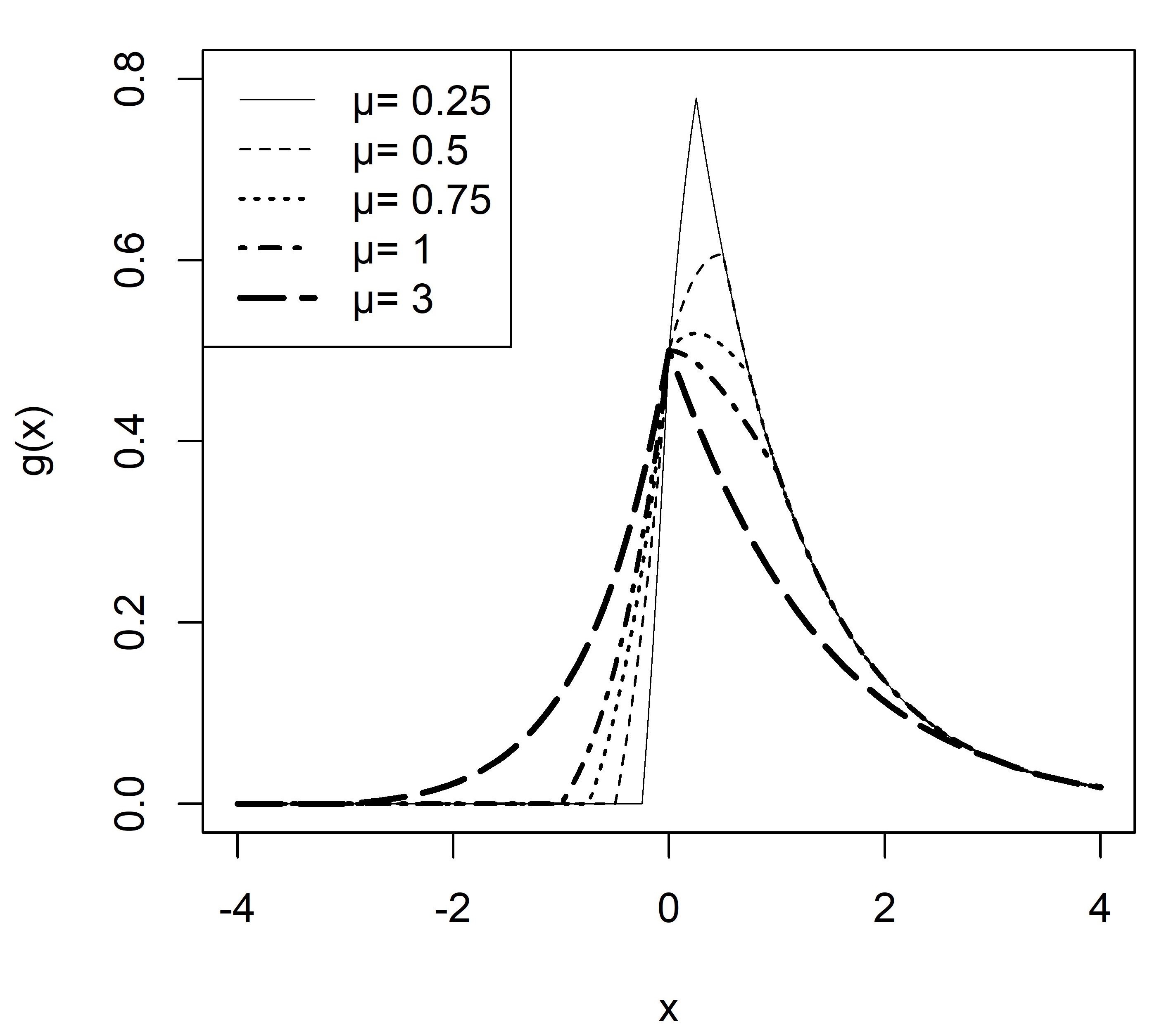
Throughout the rest of this paper, unless otherwise stated, we shall assume that , i.e., , since the corresponding results for , i.e., , can be obtained using the fact that has a pdf given by . Figure 1 illustrates the shape of the pdf (6) for .
The skew-symmetric-Laplace-uniform distribution with parameter , appears not to have been introduced yet. We provide a comprehensive description of the mathematical properties of (6). This paper follows up on Nadarajah, (2009), where a comprehensive description of the mathematical properties for the skew-logistic distribution is provided. Here, we have derived formulas for moment generating function, characteristic function, and first four raw moments (Sect. 2), mode and median (Sect. 3), hazard rate function (Sect. 4), mean deviation about ‘’ (Sect. 5), Rènyi entropy and Shannon entropy (Sect. 6), simulation and estimation by the methods of moments and maximum likelihood (Sect. 7). We also discuss these estimators’ finite sample and asymptotic properties (Sect. 7). Finally, the application of to real-life data on the daily percentage change in the price of NIFTY 50, an Indian stock market index, is discussed. Comparison of fitting of is done with fitting of normal distribution , Laplace distribution , and skew-Laplace distribution for the above data (Sect. 8).
2 Moment generating function, characteristic function, and moments
Here, we derive the moment generating function and the characteristic function of r. v. having pdf given in (6). The moment generating function (MGF) is . By using (6), one obtains
| (8) |
The corresponding characteristic function defined by is given as
| (9) |
where is the complex imaginary unit.
The moments of a probability distribution are a collection of descriptive constants used for measuring its properties. Here, we derive the expression of the first four raw moments of . They are as follows.
| (10) |
We see that for and corresponding central moments can be obtained using these raw moments but can not be simplified further. Note that, expressions given in (10) are valid only for . If , one must replace by in each of these expressions; in addition, the expressions for the odd order moments must be multiplied by -1.
(d) Kurtosis() for
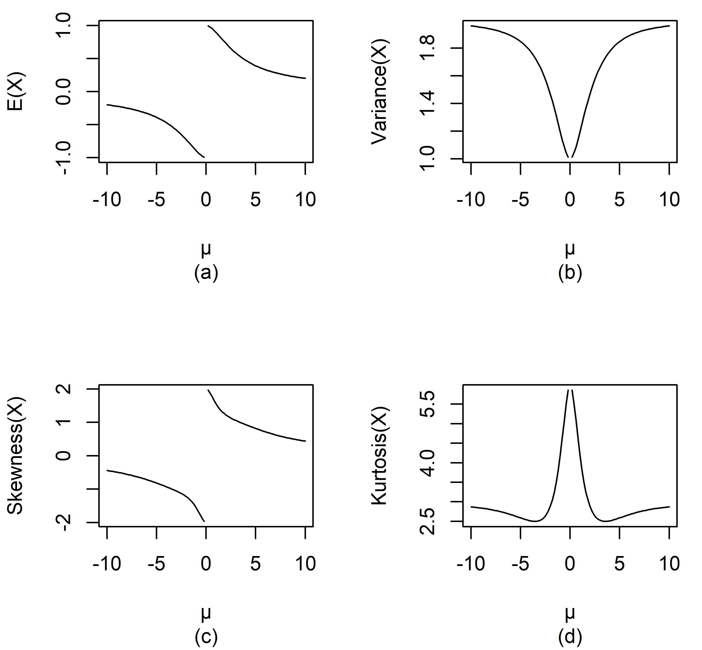
Figure 2 illustrates the behavior of the four measures E(), Var(), Skewness() and Kurtosis() for . Mean and skewness are decreasing functions of over the range and , while variance and kurtosis are even functions of . The variance strictly decreases as moves from to 0 and increases as moves from 0 to .
3 Mode and median
Mode is the value of the r. v. at which pdf is maximum. When , is,
| (11) |
It is clear from (11) that the function is increasing in and decreasing in . Hence, mode of (6) lies in the interval . Accordingly, we equate to zero and solve for x. Thus, the value of is for . But when , the function increases in and decreases in . Hence, . Similarly, when , the function increases in and decreases in . Hence, . On similar lines, one can derive the expression of for . Thus, combining these two expressions of , we get
| (12) |
| (13) |
where and . Table 1 represents values of the median of (6) for different positive values of using the Newton-Raphson iterative procedure in R-software. If , one can obtain the median on similar lines using (7a).
| 0.25 | 0.5 | 0.75 | 1 | 1.25 | 1.5 | |
|---|---|---|---|---|---|---|
| 0.6931472 | 0.6931472 | 0.6920484 | 0.6681079 | 0.6273646 | 0.5811654 |
4 Hazard rate function
The reliability function for is obtained using (7b) as,
| (14) |
The hazard rate function is an important quantity, characterizing life phenomena. After some simple steps, one can get the hazard function for as follows.
| (15) |
One can easily check that is increasing function of for as well as for . Hence, is increasing failure rate (IFR) distribution.
5 Mean deviation
The amount of scatter in a population is evidently measured to some extent by the totality of deviations from the mean and median. These are known as the mean deviation about the mean and the mean deviation about the median, respectively. Mean deviation about an arbitrary real number ‘’ is defined by .
It leads to expression as
| (16) |
To obtain mean deviation about mean and mean deviation about median, ‘’ in the above expression can be replaced by mean and median, respectively.
6 Entropy
The entropy of a random variable measures the variation of uncertainty. The Rènyi entropy of order is
| (17) |
Therefore,
| (18) |
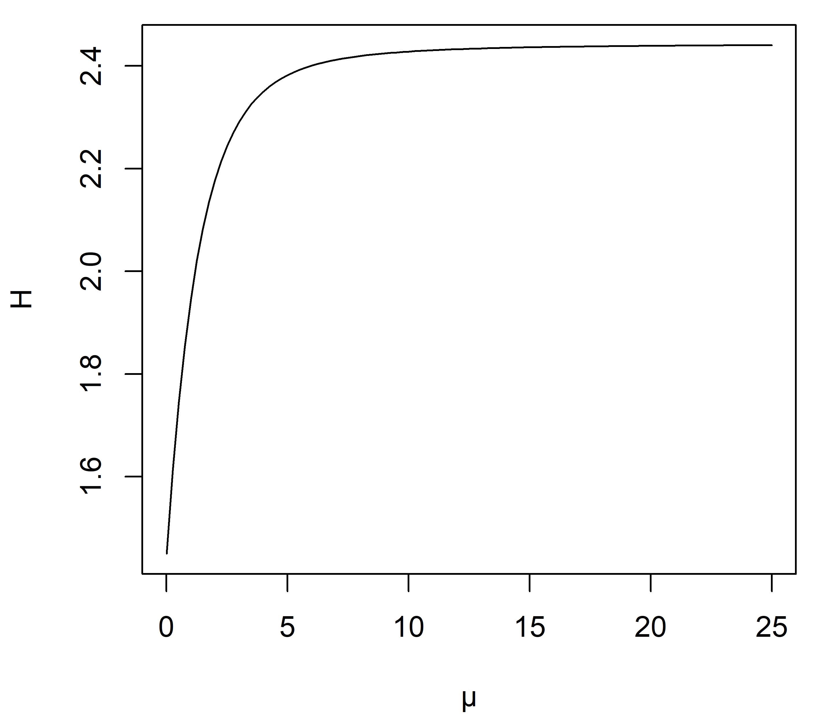
The Shannon entropy function is the particular case of (17) for , and it is , where is pdf of random variable . Using this definition, after some simplification we get,
| (19) |
Since the above integration is cumbersome, we numerically evaluate for different values of using R-software. Figure 3 represents a graph of versus .
7 Estimation
Here, we first consider simulating values of a random variable with the pdf (6) using the inverse transformation technique. Let be a random number between zero and one. The generator to generate a random sample is
| (20) |
One can use the Newton-Raphson method to solve the equation in (20) and generate a random sample from given in (6).
Now, we consider the estimation of by the method of moments and the method of maximum likelihood. To estimate unknown parameter , we have to consider both the cases and together. Suppose is an observed random sample of size ‘’ from (6). For the method of moments estimation, after equating sample mean to the first population raw moment of (6), one obtains the equation
| (21) |
From Figure 2, we see that decreases from 0 to -1 when and it decreases from 1 to 0 when , i.e., always . Therefore, if or for a particular sample, then (21) will not have an exact solution. As per Figure 2, corresponds to the closest value of to if or is a value close to zero. But as per parameter space, can not take the value zero. Hence, we define the moment estimator of as if and if . Thus, the moment estimator of is obtained as follows.
| (22) |
We consider the estimation of by the method of maximum likelihood in the following. Let be the order statistics of given sample. Suppose and ‘’ denotes the number of observations less than such that , i.e. where . Similarly, suppose and ‘’ denotes the number of observations lying in the interval such that , i.e. where . Hence, the log-likelihood function of is written as
| (23) |
In the following, we give a step-wise procedure for computation of the MLE of .
-
Step 1:
Numerically maximize over the range . Suppose the maximum value of is which is attained at , say, where ‘’ is a sufficiently large positive number chosen for computation purposes.
-
Step 2:
Numerically maximize over the range . Suppose the maximum value of is which is attained at , say.
-
Step 3:
MLE of is
(24)
Finite sample properties of and are studied using simulation, and computations are done using R- software. Table 2 and Table 3 presents bias and MSE of and for and for . We see that bias and MSE decrease as sample size increases for both MLE and moment estimator , with few exceptions only for bias. Further, the MSE of is always less than the corresponding MSE of . Also, one can observe that sign of bias of MLE is opposite to the sign of parameter . As parameter approaches zero from any side, MSE and magnitude of bias of decrease. But, no such observation in the case of the moment estimator . To check the asymptotic nature of the distribution of and using simulation, we plotted observed densities for various values of the sample size . We observe that as increases, the distribution of both and converges to the normal distribution, but the rate of convergence to normal distribution seems to be much higher for than . Thus, based on all the above results, we conclude that MLE is better than the moment estimator of for SSLUD().
| MLE | Moment estimator | ||||
|---|---|---|---|---|---|
| Bias | MSE | Bias | MSE | ||
| -1.5 | 100 | 0.06024381 | 0.045176654 | 0.0003797204 | 0.50541564 |
| 200 | 0.03906522 | 0.021357856 | 0.0157055747 | 0.26786436 | |
| 300 | 0.02933963 | 0.012989993 | -0.0008644177 | 0.16465504 | |
| 400 | 0.02375948 | 0.009209691 | -0.0085926100 | 0.12896987 | |
| 500 | 0.01766114 | 0.007451091 | -0.0065899772 | 0.10033671 | |
| 600 | 0.01808905 | 0.006370478 | 0.0075580998 | 0.08311324 | |
| 700 | 0.01456689 | 0.005214147 | -0.0003676365 | 0.06853064 | |
| 800 | 0.01492506 | 0.004456640 | -0.0164346584 | 0.05661172 | |
| 900 | 0.01381575 | 0.003861085 | -0.0079539753 | 0.05188121 | |
| 1000 | 0.01378036 | 0.003294051 | 0.0052817371 | 0.04687188 | |
| -0.75 | 100 | 0.032511901 | 0.0134889603 | -0.02488011 | 0.37927153 |
| 200 | 0.023375017 | 0.0062341973 | 0.02678563 | 0.24807994 | |
| 300 | 0.022614234 | 0.0040753483 | 0.05442608 | 0.18159122 | |
| 400 | 0.013782428 | 0.0026481775 | 0.02407104 | 0.14540491 | |
| 500 | 0.014188578 | 0.0019942288 | 0.04011415 | 0.12661616 | |
| 600 | 0.010531113 | 0.0016580024 | 0.02741234 | 0.10965835 | |
| 700 | 0.009567891 | 0.0014142729 | 0.02247448 | 0.09215384 | |
| 800 | 0.008969822 | 0.0012107034 | 0.03299546 | 0.08416938 | |
| 900 | 0.008833928 | 0.0010258905 | 0.02604549 | 0.07738691 | |
| 1000 | 0.007307065 | 0.0009473139 | 0.01597401 | 0.06532169 | |
| -0.25 | 100 | 0.026910685 | 0.0043941552 | -0.20148295 | 0.28701317 |
| 200 | 0.014633591 | 0.0016442189 | -0.12561277 | 0.18340413 | |
| 300 | 0.011298482 | 0.0010134272 | -0.11008763 | 0.14648063 | |
| 400 | 0.008403715 | 0.0007178242 | -0.07115405 | 0.11693260 | |
| 500 | 0.006866262 | 0.0005193217 | -0.05475621 | 0.10104767 | |
| 600 | 0.006577965 | 0.0004359336 | -0.04101810 | 0.09227325 | |
| 700 | 0.005574953 | 0.0003294627 | -0.03931742 | 0.08363312 | |
| 800 | 0.005196938 | 0.0002914057 | -0.02245561 | 0.07867760 | |
| 900 | 0.004681950 | 0.0002552058 | -0.03305608 | 0.07551096 | |
| 1000 | 0.003797666 | 0.0002160883 | -0.01393033 | 0.06746986 | |
| MLE | Moment estimator | ||||
|---|---|---|---|---|---|
| Bias | MSE | Bias | MSE | ||
| 0.25 | 100 | -0.026141601 | 0.0040926127 | 0.19908173 | 0.30299408 |
| 200 | -0.015706993 | 0.0017378035 | 0.11979148 | 0.18277572 | |
| 300 | -0.010537695 | 0.0009629724 | 0.10281278 | 0.15122684 | |
| 400 | -0.009388154 | 0.0006823647 | 0.07138595 | 0.11273918 | |
| 500 | -0.007654403 | 0.0005241705 | 0.06670007 | 0.10613451 | |
| 600 | -0.006541976 | 0.0004273222 | 0.04710248 | 0.09317236 | |
| 700 | -0.005775066 | 0.0003498924 | 0.03681952 | 0.08264223 | |
| 800 | -0.005424833 | 0.0003076071 | 0.02613340 | 0.07893736 | |
| 900 | -0.004687041 | 0.0002641379 | 0.02308814 | 0.07288723 | |
| 1000 | -0.004587965 | 0.0002188929 | 0.02168387 | 0.07098162 | |
| 0.75 | 100 | -0.039403641 | 0.0141163154 | 0.02381151 | 0.36120747 |
| 200 | -0.023215667 | 0.0057148979 | -0.01903135 | 0.24011612 | |
| 300 | -0.018010206 | 0.0037173032 | -0.04910507 | 0.18917471 | |
| 400 | -0.013004298 | 0.0026953723 | -0.02435556 | 0.13988301 | |
| 500 | -0.011937422 | 0.0020292707 | -0.04849263 | 0.13064004 | |
| 600 | -0.010423756 | 0.0016294899 | -0.02277927 | 0.10673985 | |
| 700 | -0.009229675 | 0.0013339162 | -0.03201923 | 0.09343322 | |
| 800 | -0.009286969 | 0.0011661790 | -0.02381294 | 0.08053673 | |
| 900 | -0.008850638 | 0.0010360152 | -0.02366172 | 0.07657251 | |
| 1000 | -0.008957869 | 0.0009469547 | -0.01562601 | 0.06498910 | |
| 1.5 | 100 | -0.05884554 | 0.047383765 | -0.013127745 | 0.54926083 |
| 200 | -0.03000957 | 0.020339855 | -0.006090958 | 0.25400260 | |
| 300 | -0.03186303 | 0.013144354 | -0.010153344 | 0.16976755 | |
| 400 | -0.02284458 | 0.009625618 | -0.002482506 | 0.13057787 | |
| 500 | -0.02293975 | 0.007759937 | -0.008421723 | 0.09775602 | |
| 600 | -0.01841574 | 0.005969112 | -0.009321518 | 0.08234397 | |
| 700 | -0.01724714 | 0.005152509 | -0.004056375 | 0.06780765 | |
| 800 | -0.01197158 | 0.004282729 | -0.008411236 | 0.06338525 | |
| 900 | -0.01484989 | 0.004060138 | -0.009773787 | 0.05273530 | |
| 1000 | -0.01228560 | 0.003408502 | 0.003389947 | 0.04925195 | |
8 Application
In this section, we present the application of skew-symmetric-Laplace-uniform distribution for modeling daily percentage change in the price of NIFTY 50, an Indian stock market index. Further, we have fitted and compared the proposed distribution with normal distribution , Laplace distribution , and skew-Laplace distribution for percentage change data. Here, refers to a special case of skew-Laplace distribution using and as pdf and cdf of standard Laplace distribution in (1). The NIFTY 50 is a benchmark Indian stock market index representing the weighted average of 50 of the largest Indian companies listed on the National Stock Exchange (NSE). It is one of the two leading stock indices used in India. The daily price of NIFTY 50 quoted in the National Stock Exchange of India Ltd. is available at https://in.investing.com/indices/s-p-cnx-nifty-historical-data and is selected for the current study. We consider the daily percentage change on day t given by , where denotes the price of NIFTY 50 on day t. This transformed data covering the period December 2021 to April 2022 (82 working days) is as follows :
0.16, - 1.53, - 2.18, 0.94, 1.10, 0.69, - 0.40, 0.49, 0.86, - 0.11, - 0.06, 0.87, 1.57, 1.02, 0.67, - 1.00, 0.38, 1.07, 0.29, 0.87, 0.25, - 0.01, 0.29, - 1.07, - 0.96, - 1.01, - 0.79, - 2.66, 0.75, - 0.97, - 0.05, 1.39, 1.37, 1.16, - 1.24, - 0.25, - 1.73, 0.31, 1.14, 0.81, - 1.31, - 3.06, 3.03, - 0.17, - 0.10, - 0.16, - 0.40, - 0.67, - 0.17, - 4.78, 2.53, 0.81, - 1.12, - 0.65, - 1.53, - 2.35, 0.95, 2.07, 1.53, 0.21, 1.45, - 1.23, 1.87, 1.84, - 0.98, 1.16, - 0.40, - 0.13, - 0.40, 0.40, 0.60, 1.00, - 0.19, 1.18, 2.17, - 0.53, - 0.83, - 0.94, 0.82, - 0.62, - 0.82, - 0.31.
Mean, variance, and skewness for the above data is 0.027, 1.671, and - 0.639 respectively. The Wald-Wolfowitz runs test for randomness of yields a p-value of 0.076, justifying the assumption of independence of the values. We consider fitting the proposed skew-symmetric-Laplace-uniform distribution along with normal distribution , Laplace distribution , and skew-Laplace distribution to the data on percentage change. Using R-software, the MLE of the parameters and hence, the estimated value of log-likelihood are obtained. Akaike’s Information Criteria (AIC) and Bayesian Information Criteria (BIC) are used for model comparison. Table 4 shows that the proposed provides the best fit for the data set which is very close to in terms of BIC. But in terms of AIC, N() seems to be better than and the best among the four distributions.
| Distribution | MLEs | ln | AIC | BIC |
|---|---|---|---|---|
| = 62.38674 | - 138.7604 | 279.5207 | 281.9274 | |
| = -6.247468e-05 | - 138.7782 | 279.5564 | 281.9631 | |
| = - 0.03 , = 0.9990244 | - 138.7580 | 281.5161 | 286.3295 | |
| = 0.02682927, = 1.650275 | - 136.9081 | 277.8162 | 282.6296 |
For , MLE of is =62.38674 which is relatively high, and by definition of in (6) for a large value of , SSLUD approaches to Laplace distribution. But, from the histogram in Figure 4 and the value of skewness for , one can observe that data is negatively skewed. It might be due to a single parameter in the proposed distribution unable to give the best fit to the data. By changing the data location, significant change observed in SSLUD’s curve in terms of location, scale, and shape. So, by observation, one can choose an appropriate change in location such that the value of is significantly small for possible better fitting of data using the proposed distribution. Through the trial and error method, here we consider a change as - 0.8 and define transformed daily percentage change in Nifty 50 index price, which gives , a significantly small value. A possible generalization of proposed distribution with additional location parameter to avoid hindrance to employ it is under consideration, in order to make it more flexible and apt to catch the features present in real data.
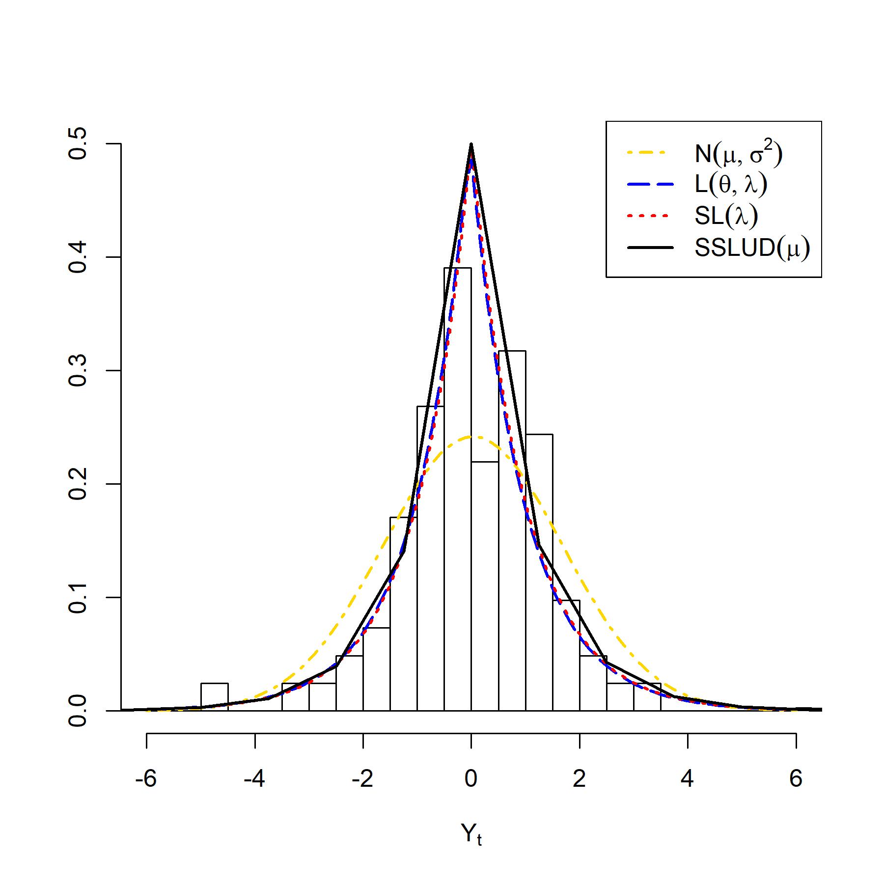
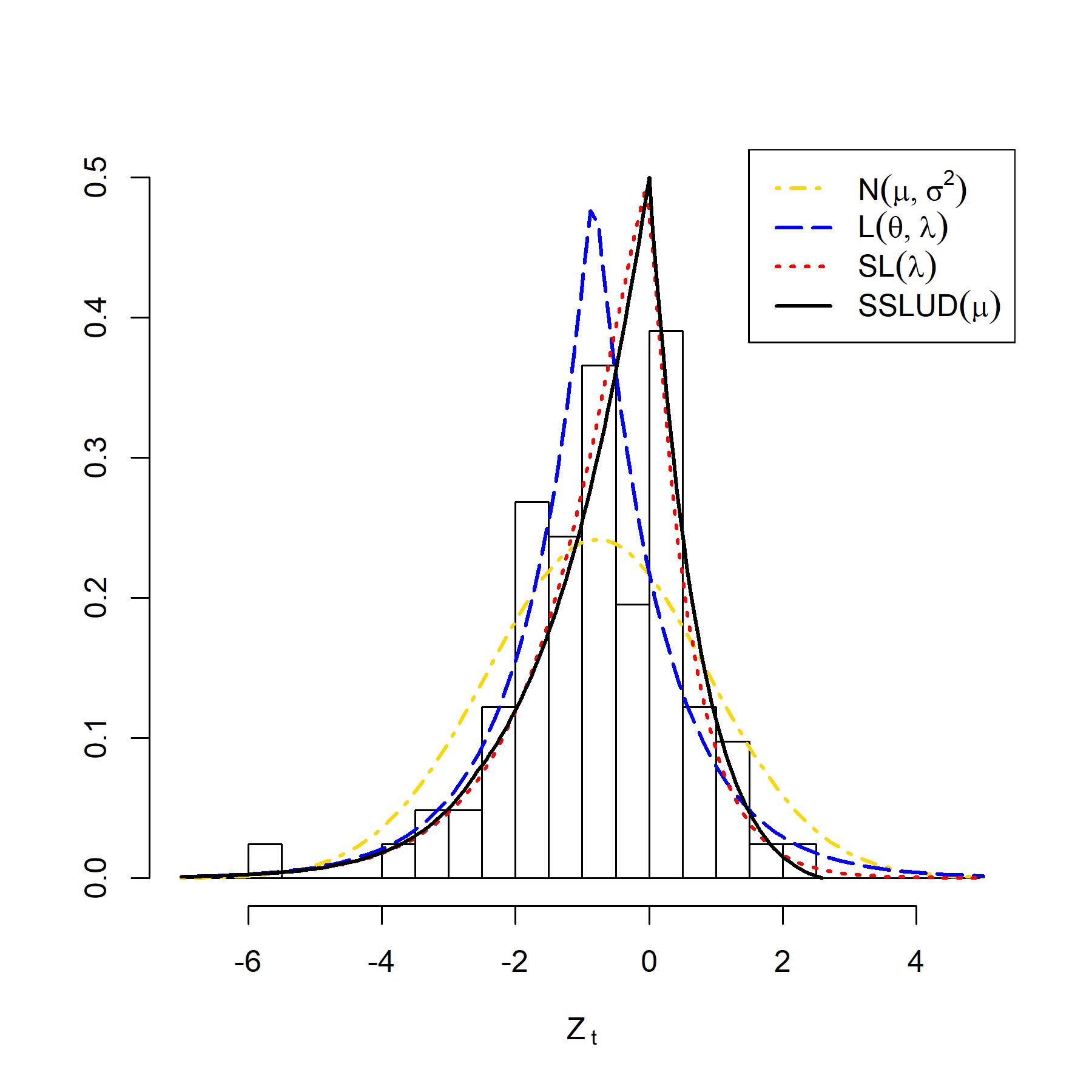
Table 5 shows the MLEs, estimated log-likelihood, AIC, and BIC by fitting the distributions mentioned above to . The graphical representation of the results is given in Figure 5. It is clear from Table 5 that the proposed provides the best fit for the data set in terms of both AIC and BIC, but close to . The plot of observed and expected densities presented in Figure 5 also confirms our findings. Thus, is better for modeling daily percentage change in the price of NIFTY 50 in comparison to normal distribution and Laplace distribution , and one good alternative to skew-Laplace distribution .
| Distribution | MLEs | ln | AIC | BIC |
|---|---|---|---|---|
| = - 2.589259 | - 136.8343 | 275.6685 | 278.0752 | |
| = - 0.6988722 | - 137.0020 | 276.0040 | 278.4107 | |
| = - 0.83 , = 0.9990244 | - 138.7580 | 281.5161 | 286.3295 | |
| = - 0.7731707, = 1.650275 | - 136.9081 | 277.8162 | 282.6296 |
Declarations
Conflict of interest
The authors declare that they have no conflict of interest to disclose.
Ethics approval and consent to participate
Not applicable.
Consent for publication
Both authors have agreed to submit and publish this paper.
References
- Arnold and Lin, (2004) Arnold, B. C. and Lin, G. D. (2004). Characterizations of the skew-normal and generalized chi distributions. Sankhyā: The Indian Journal of Statistics, 66(4):1–14.
- Aryal and Rao, (2005) Aryal, G. and Rao, A. (2005). Reliability model using truncated skew-laplace distribution. Nonlinear Analysis, 63:e639–e646.
- Azzalini, (1985) Azzalini, A. (1985). A class of distributions which includes the normal ones. Scandinavian journal of statistics, 12(2):171–178.
- Kotz et al., (2001) Kotz, S., Kozubowski, T., and Podgórski, K. (2001). The Laplace distribution and generalizations: a revisit with applications to communications, economics, engineering, and finance. Springer Science & Business Media.
- Kozubowski and Nolan, (2008) Kozubowski, T. J. and Nolan, J. P. (2008). Infinite divisibility of skew gaussian and laplace laws. Statistics & probability letters, 78(6):654–660.
- Kozubowski and Podgórski, (2001) Kozubowski, T. J. and Podgórski, K. (2001). Asymmetric laplace laws and modeling financial data. Mathematical and Computer Modelling, 34:1003–1021.
- Nadarajah, (2009) Nadarajah, S. (2009). The skew logistic distribution. Advances in Statistical Analysis, 93:187–203.
- Nadarajah and Kotz, (2003) Nadarajah, S. and Kotz, S. (2003). Skewed distributions generated by the normal kernel. Statistics & probability letters, 65(3):269–277.
- Nekoukhou and Alamatsaz, (2012) Nekoukhou, V. and Alamatsaz, M. (2012). A family of skew-symmetric-laplace distributions. Statistical papers, 53:685–696.
- Rachev and SenGupta, (1993) Rachev, S. and SenGupta, A. (1993). Laplace-weibull mixtures for modeling price changes. Management Science, 39(8):1029–1038.
- Rydén et al., (1998) Rydén, T., Teräsvirta, T., and Åsbrink, S. (1998). Stylized facts of daily return series and the hidden markov model. Journal of applied econometrics, 13(3):217–244.
- Theodossiou, (1998) Theodossiou, P. (1998). Financial data and the skewed generalized t distribution. Management Science, 44(Part 1 of 2):1650–1661.
- Zeckhauser and Thompson, (1970) Zeckhauser, R. and Thompson, M. (1970). Linear regression with non-normal error terms. The Review of Economics and Statistics, 52:280–286.