The small-scale dynamo in a multiphase supernova-driven medium
Abstract
Magnetic fields grow quickly, even at early cosmological times, suggesting the action of a small-scale dynamo (SSD) in the interstellar medium (ISM) of galaxies. Many studies have focused on idealized, isotropic, homogeneous, turbulent driving of the SSD. Here we analyze more realistic simulations of supernova-driven turbulence to understand how it drives an SSD. We find that SSD growth rates are intermittently variable as a result of the evolving multiphase ISM structure. Rapid growth in the magnetic field typically occurs in hot gas, with the highest overall growth rates occurring when the fractional volume of hot gas is large. SSD growth rates correlate most strongly with vorticity and fluid Reynolds number, which also both correlate strongly with gas temperature. Rotational energy exceeds irrotational energy in all phases, but particularly in the hot phase while SSD growth is most rapid. Supernova (SN) rate does not significantly affect the ISM average kinetic energy density. Rather, higher temperatures associated with high SN rates tend to increase SSD growth rates. SSD saturates with total magnetic energy density around 5% of equipartition to kinetic energy density, increasing slightly with magnetic Prandtl number. While magnetic energy density in the hot gas can exceed that of the other phases when SSD grows most rapidly, it saturates below 5% of equipartition with kinetic energy in the hot gas, while in the cold gas it attains 100%. Fast, intermittent growth of the magnetic field appears to be a characteristic behavior of SN-driven, multiphase turbulence.
1 Introduction
Magnetic fields pervade the Universe at all scales. Many astrophysical systems consist of plasma, in which the highly turbulent motions drive small-scale dynamos (SSD) that rapidly grow magnetic fluctuations at the scales characteristic of the turbulence. Such magnetic fields influence the structure and dynamics of, for example, star forming molecular clouds (Mac Low & Klessen, 2004; van Loo et al., 2012; Federrath & Klessen, 2012; Sridharan et al., 2014) and spiral arms (Chandrasekhar & Fermi, 1953; Beck et al., 1996; Fletcher et al., 2011). Magnetic fields also grow at larger scales relevant to the shape and structure of their host, such as the polar fields in stars aligned to the rotational axis, or galactic fields aligned to the spiral arms or disk (e.g., Harnett et al., 2004; Fletcher et al., 2011; Beck, 2016). Such fields are generated by large-scale dynamos (LSDs). To model galactic LSDs self-consistently (e.g., Gressel et al., 2008; Hanasz et al., 2009; Gent et al., 2013b) requires its evolving entanglement with the SSD be included. The vast separation in scale and growth time makes this challenging.
The SSD has been investigated numerically for astrophysically relevant parameters, such as low magnetic Prandtl number Pm applying to the Sun or stars (e.g., Schekochihin et al., 2005; Iskakov et al., 2007; Brandenburg, 2011; Warnecke et al., 2022), high Pm typical of the interstellar medium (ISM) or intracluster medium (e.g., Schekochihin et al., 2002; Schober et al., 2012; Seta et al., 2020), and high sonic Mach number (e.g., Haugen et al., 2004; Federrath et al., 2011, 2014), which would apply in turbulence driven by supernova (SN) explosions.
Amplification and decay of magnetic fluctuations in highly compressible fluids can occur independent of the presence of an SSD through a process called tangling, where a large-scale field is pushed around by the turbulent flow, and a fluctuating contribution is generated (Rogachevskii & Kleeorin, 2007; Karak & Brandenburg, 2016). In regions of SN compression, magnetic field strength scales with density, the exponent of its proportionality depending on the geometry of the compression. However, observations of the diffuse ISM show no correlation between field strength and density (e.g., Crutcher et al., 2003). Observations of galaxies indicate that the turbulent magnetic field strength is typically larger than that of the large-scale fields. The Solar neighbourhood random field, for example, is about 1.3 times larger than the local regular field (Beck et al., 2003). These fields are roughly in equipartition with the estimated turbulent kinetic energy density.
It is somewhat uncertain how LSD, tangling and SSD interact and contribute to this picture. Based on a suite of numerical experiments, Karak & Brandenburg (2016) reported that while tangling, as expected, is positively correlated with the large scale magnetic fields, the SSD shows an anti-correlation when the mean component of the magnetic field becomes strong. Super-equipartition mean fields, which could arise in presence of fluxes of small scale magnetic helicity, tend to suppress SSD. Some properties of tangling produced magnetic fluctuations are discussed in Gent et al. (2021) where it was noted that tangling produces only a linear growth for a given background mean magnetic field. If the background field itself grows exponentially, the associated fluctuations by tangling are also expected to show an exponential growth. However, in the absence of any regular or mean magnetic field, as is the case in the present work, exponentially growing solutions for small scale magnetic fields must be attributed to SSD.
The high resolution simulations of Bhat et al. (2016) include SSD and LSD simultaneously, but only for isothermal, helically-driven turbulence at . Galaxy simulations including halo-disk scale flows (e.g., Rieder & Teyssier, 2016; Steinwandel et al., 2019) find SSD but capture no LSD. Their multiphase structure is parameterized, not evolved explicitly. While lower resolution models of LSD in SN-driven turbulence with galactocentric differential rotation do not include SSD, Gent et al. (2013b) appeared to do so in a non-isothermal model, as confirmed by Gent et al. (2021). We do not yet investigate the interaction of the LSD and SSD here, but examine only the properties of the SSD.
Seta & Federrath (2022) model SSD in a two-phase ISM (cold and warm) using large-scale momentum injection to drive the turbulence, rather than point-source thermal injection as primarily applied here. In the case of both solenoidal and compressive forcing they find a large dispersion in the correlation of magnetic field strength to gas density (see their Figure 5). Compressive forcing yields a perceptible trend of for warm gas, and for cold, consistent with the relations for compression along field lines and spherically, respectively.
SSD in the cold and warm phases has the same growth rate in Seta & Federrath (2022). Their cold gas has typically higher , so, based on their previous isothermal models (Seta & Federrath, 2021), SSD should be slower. Overall growth is slower in the multiphase medium than in an isothermal gas of similar mean . Separation into cold and warm phases driven by thermal instability (Field et al., 1969; Sánchez-Salcedo et al., 2002; Brandenburg et al., 2007; McCourt et al., 2012). The Seta & Federrath (2021) cooling function has a slightly reduced range of instability than what we model here. Of greater significance is that without SN thermal energy injection they also have no hot gas in a quasi-stable third phase (McKee & Ostriker, 1977). The models we present here suggest this is a crucial difference.
The SSD in SN-driven turbulence has been modelled by Balsara et al. (2004) and Gent et al. (2021). The second of these included a multi-phase ISM with fractional volumes of cold, warm and hot gas somewhat consistent with observations. Their key finding was to confirm that under the conditions prevailing in an ISM heated by SNe, the SSD is easy to excite and amplifies magnetic fluctuations up to sub-equipartition levels within a few tens of megayears. A critical issue that was not resolved, though, was to explain the erratic growth rate of the dynamo in these simulations, which was not observed by Balsara et al. (2004).
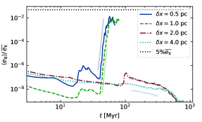
We illustrate this intermittent dynamo in Figure 1 where we reproduce data from Gent et al. (2021) Figure 3, but with the inclusion of least-squares fits of magnetic energy density . False convergence (Fryxell et al., 1991) is apparent at low resolution, although the 2 pc resolution model does exhibit a brief spell of growth at around 200 megayears. At high resolution the solutions are convergent at all times, with slightly more diffusivity apparent at 1 pc resolution. Of interest for our study is the sporadic growth and decay apparent at high resolution between 20 and 40 megayears, and to some degree also after 50 megayears. In particular, we seek to understand how the SSD in the multiphase ISM differs from solutions modelled in isothermal plasmas, and to explain how this drives such intermittency in SSD behaviour. In Gent et al. (2021) only the volume averaged growth rates were considered. In results presented here we include a breakdown by phase.
In Section 2 we explain the motivation and design of our experiments. In Section 3 we report on the key drivers that change SSD growth within and between models. This includes consideration of how magnetic Prandtl number varies in the multiphase environment of the ISM. We conclude with a discussion of the significance of these results in Section 4.
| Model | resolution | ||||||||||||||
|---|---|---|---|---|---|---|---|---|---|---|---|---|---|---|---|
| [pc] | [] | [kpc km s-1] | [kpc km s-1] | ||||||||||||
| UP0r10sl | 0.5 | 0.2 | 0.0 | 1.6 | |||||||||||
| HP0r10sl | 1.0 | 0.2 | 0.0 | 3.5 | |||||||||||
| HP1r10sl | 1.0 | 0.2 | 2.5 | ||||||||||||
| HP2r5sl | 1.0 | 0.2 | 2.5 | ||||||||||||
| HP5r2sl | 1.0 | 0.2 | 2.5 | ||||||||||||
| HP5r8sm | 1.0 | 0.5 | 2 | ||||||||||||
| MP0r10sl | 2.0 | 0.2 | 0.0 | 8.25 | |||||||||||
| MP2r5sl | 2.0 | 0.2 | 8.25 | ||||||||||||
| MP0r10sh | 2.0 | 1.0 | 0.0 | 8.25 | |||||||||||
| MP0r5sh | 2.0 | 1.0 | 0.0 | 8.25 | |||||||||||
| LP0r10sl | 4.0 | 0.2 | 0.0 | 2 | |||||||||||
| LP2r5sl | 4.0 | 0.2 | 2 | ||||||||||||
| LP5r8sm-S | 4.0 | 0.5 | 1 | ||||||||||||
| LP0r10sh | 4.0 | 1.0 | 0.0 | 2 | |||||||||||
| LP0r5sh | 4.0 | 1.0 | 0.0 | 2 |
2 Method
2.1 MHD equations
We use the Pencil Code (Brandenburg & Dobler, 2002; Brandenburg et al., 2020) to model SN-driven turbulence as described previously in Gent (2012), Gent et al. (2013a), and Gent et al. (2020). We solve the system of nonideal, compressible, nonadiabatic, MHD equations
| (1) | |||||
| (2) | |||||
| (3) | |||||
| (4) | |||||
with the ideal gas equation of state closing the system, assuming an adiabatic index (ratio of specific heats) . Most variables take their usual meanings; a list of notations used is given in Table 2.
| Symbol | Denoting | Units/Definition |
|---|---|---|
| magnetic energy density | [erg cm-3] | |
| time-averaged kinetic energy density | [erg cm-3] | |
| volume-averaged growth rate | [Gyr-1] | |
| relative growth rate | [Gyr-1] | |
| absolute growth rate | [Gyr-1] | |
| SN explosion rate | [kpc-3 Myr-1] | |
| material derivative | ||
| gradient vector | e.g., | |
| gas density | [g ] | |
| gas velocity | [km s-1] | |
| time | [Myr] | |
| specific entropy | [erg g-1 K-1] | |
| gas temperature | [K] | |
| magnetic vector potential | [G cm] | |
| magnetic field | [G] | |
| current density | [erg cm-4 G-1] | |
| W | traceless rate of strain tensor | |
| contraction of W | ||
| 6th order rate of strain tensor | ||
| shock diffusion coefficients | ||
| viscosity, resistivity coefficients | [kpc km s-1] | |
| hyperdiffusion coefficients | [kpc5 km s-1] | |
| UV-heating | [erg g-1 s-1] | |
| radiative cooling | [erg cm3 g-2 s-1] | |
| SN explosion energy | [1051erg] | |
| vacuum magnetic permeability | 1 | |
| sound speed | [km s-1] | |
| specific heat at constant pressure | [erg g-1 K-1] | |
| specific heat at constant volume | [erg g-1 K-1] |
Terms containing and apply sixth-order hyperdiffusion to resolve grid-scale instabilities (see, e.g., Brandenburg & Sarson, 2002; Haugen & Brandenburg, 2004), with mesh Reynolds number set to be at the scale of the zone size . Terms including and resolve shock discontinuities with artificial diffusion of mass, momentum, and thermal energy, respectively. They depend quadratically on the local strength of the shock (see Gent et al., 2020, for details). Equations (2) and (4) include momentum and energy conserving corrections for the artificial mass diffusion applying in Equation (1). Following Gent et al. (2021), resistive shock diffusion is omitted from Eq. (3).
2.2 Model parameters
We simulate a nonstratified, nonrotating domain with initial gas number density covering (256 pc)3 and periodic across all boundaries. Resolution along each edge spans 0.5 to , corresponding to grid sizes of to zones. Each model SN rate is given relative to the estimated rate in the Solar neighbourhood of the Milky Way, . SNe occur uniform randomly in space at times following a Poisson process. Models with common use the same SN schedule and locations. For ambient gas number density and an estimated forcing scale of 60–100 pc (Joung & Mac Low, 2006; de Avillez & Breitschwerdt, 2007; Hollins et al., 2017) should support at least 2–4 turbulent cells. For higher SN rates the forcing scale reduces, increasing the number of turbulent cells (Joung et al., 2009), but the forcing scale remains unchanged for the lower SN rates applying here, where an individual SN at gas number density merges with the local sound speed within a 70 pc radius (Gent et al., 2020)
In addition, Model LP5r8sm-S, is vertically stratified without rotation and has open vertical boundaries. Initially at the midplane. With this we examine the effect that vertical expansion of SN remnants or superbubbles has on the SSD. Here is amplified to that of Wolfire et al. (1995) to support the thickness of the disk in the absence of ionization heating and cosmic ray pressure gradients (see Hill et al., 2018). The domain size of this model is along the disk and perpendicular to it. SN are located uniform random horizontally and normal random with scale heights of and for Type I and Type II SNe, respectively (Ferrière, 2001). This model otherwise is as described in Gent et al. (2013a, b).
All models are listed in Table 1 where the model labelling convention is explained.
2.3 Averaging conventions
Angular brackets indicate the quantity is averaged over the volume, or also with a subscript when over the volume of individual temperature phases. An overbar indicates averaging over a domain and an interval of time, intervals which may vary, as explained in the text.
In the case of the interval is selected for each model to exclude initial transients and the period after the SSD approaches saturation. Even with saturation around 5% of equipartition energy, some models show damping in kinetic energy. Models with identical SN rates, have near identical kinetic energy density evolution, so direct comparisons are not affected by this choice. The magnetic energy density is then normalized by to ease model comparison.
2.4 Growth rates and Reynolds number
The erratic growth of the volume averaged magnetic energy shown in Figure 1 and discussed in Sect. 3 shows that the kinematic stage of the SSD does not have a well-defined single growth rate (Gent et al., 2021). SSD growth typically follows an exponential of the form
| (5) |
In Figure 1 we fit such a function to specified time intervals for each model, but the SSD growth (or decay) at other times differs, with varying or no clear exponential behaviour occurring. Indeed within the domain, we can find very different growth patterns within and between thermal phases.
To interpret how the time and volume averaged growth rate is influenced by the phases and dynamical properties, we can use Eq. (3) to identify instantaneous changes to the magnetic energy. Hyperdiffusion, being purely numerical, is neglected. Taking the curl of Eq. (3) and contracting it with , we obtain an equation for the change of the magnetic energy density
| (6) |
Negative values represent decay of the magnetic field and positive its amplification. Dividing by , we obtain an equation for the relative growth rate exponent, of the form , at each instant in time and location in space
| (7) |
Here, is a function of position , distinct from defined above, which is the volume and time averaged quantity. Statistical analysis of in relation to various physical properties will help determine how the varying growth depends on the multiphase structure of the ISM.
The growth rate does not indicate the absolute magnitude of the energy change. We also need to identify where the largest changes in magnetic energy density occur, since these need not correlate with the growth rates. We therefore also define the absolute growth rate
| (8) |
replacing in the denominator with the time dependent volume averaged . Rescaling by time dependent assists comparison between all stages of the SSD. Both and have values that span orders of magnitude of both signs. To take advantage of logarithmic scales in our histograms we omit negative and negligible growth rates.
Similarly, a field of values for the magnetic Reynolds number Rm is calculated directly from the induction equation by taking the ratio of the advection to the diffusion terms,
| (9) |
where . In a related approach, Evirgen et al. (2019) decompose the terms of Equation (2) to identify separately the spatial variation of each force.
| phase | temperature range |
|---|---|
| cold | |
| warm | |
| hot | |
| time interval | |
| 0.5 & 1 pc | |
| 2 pc | |
| 4 pc |
2.5 Phase fractional volume
There are various approaches to measuring the proportion of the ISM that contains gas in each phase, as discussed in detail within Gent et al. (2013a). Here, we measure the fractional volume of SSD activity for each phase defined as
| (10) |
where is the volume occupied by the gas in the temperature range defining phase , as listed in Table 3, and is the total volume. Both the phase volume and the total volume omit locations with negative or negligible to focus on SSD growth. For each phase, is computed from the snapshot within the time intervals listed in Table 3.
2.6 Sorting time by growth rate
To examine how properties of the ISM in each phase differ between times with rapid growth and slow growth or decay, for each model we compute the average growth rate as the rate of change in during the specified intervals from Table 3. The intervals are chosen at each resolution to exclude initial transient magnetic energy decay, prior to the onset of any SSD, and most of the subsequent saturated dynamo stage, so that we capture data of most relevance to SSD. The time series is then binned according to where is lowest, median and highest.111 Sampling only the lowest, median, and highest 5%, 15%, or 25% yielded results consistent with our method of simply splitting the growth rates into three bins.
Histograms for each phase from snapshots at times belonging to each time bin are then accumulated. Fractional volume of SSD activity for each phase for a cumulative histogram is the mean of in snapshots contributing to that histogram. Summary statistics of mean or and relevant averaged physical quantities are calculated from cumulative histograms in each bin.
3 Results
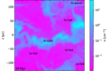
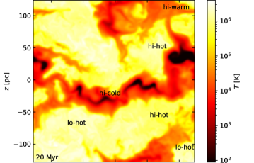
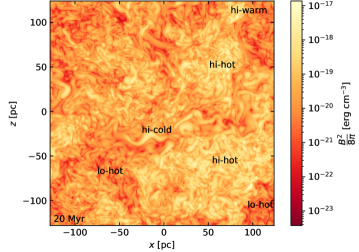
A hint toward explanation for the intermittent growth in the SSD in these models appears on inspection of slices of the simulation data as displayed in Figure 2 for Model HP2r5sl. The expected response of the magnetic energy to compressive flows is evident in regions highlighted by labels ‘hi-cold’, ‘hi-warm’ and ‘lo-hot’. What is anomalous in this scenario are the regions highlighted as ‘hi-hot’. In these regions the strongest magnetic field is associated with the most diffuse and hottest ISM. This cannot be explained by passive compression of the field and suggests strong SSD activity in these regions. The snapshot shown is at , a period in the simulation when there is a burst of magnetic field growth. Why is SSD present in these and not in other regions of hot gas, and why is field growth strong during this period and not others?
For our core analysis of the multiphase structure of the SSD we primarily focus on our models with resolution of 1 pc. We include the highest resolution 0.5 pc model to demonstrate how well our solutions converge. The lower resolution runs support insights into the dependence of the SSD on ISM structure and SN rate.
We hypothesise that the erratic behaviour of the SSD is due to the changing multiphase structure of the ISM. To test this hypothesis, we compute joint histograms by thermal phase of various physical properties in the total domain from snapshots of each model alongside growth rates computed using Equations (7) and (8).
3.1 Vorticity
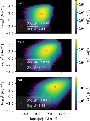
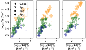
In Figure 3 we display the set of cumulative joint histograms of absolute growth and (twice the) enstrophy or the norm squared vorticity of cold, warm and hot gas from Model HP5r2sl. As is common across all models and variables, there is large variance and histograms overlap between the phases. However, a clear trend appears of increasing vorticity and growth rate with temperature. In the warm and hot phases there is discernible positive correlation between vorticity and growth rate within the phase. The phases and time intervals used for the histograms are listed in Table 3.
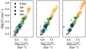
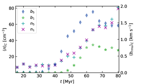
The most striking correlation we find is between relative growth rate and the norm squared vorticity , which we show in Figure 4(a). We find that the growth rate is strongly proportional to , and vorticity increases as we move from cold to hot gas at all times. At times belonging to the high growth rate bin (right panel) the hot gas increases in vorticity, while the vorticity in the cold and warm gas does not differ so much between bins. The fractional volume of the hot gas increases slightly for high resolution within the upper bin. So the efficiency of the SSD is linked to high vorticity and high local and average growth rates and are correlated with increased vorticity in the hot gas, consistent with results from models using more idealised turbulence (Federrath et al., 2011; Achikanath Chirakkara et al., 2021)
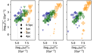
To confirm whether this correlation is reflected in the absolute gains in magnetic energy we plot the same summary for in Figure 4(b). At high resolution the same trends are preserved as for , with the changes in most associated with changes in the characteristics of the hot gas. However for low resolution is actually anti-correlated with vorticity. Increased mixing at low resolution dampens vorticity and inhibits the formation of hot gas, damping the SSD.
Energy growth at low resolution is better correlated with gas density, the cold and then warm phases exhibiting higher , consistent with results from isothermal modelling, except at for the upper bin of (right) when vorticity and fractional volume increases for the hot gas. Mean vorticity in the warm and cold phases does not change markedly between bins.
3.2 Mach number and Rm dependence
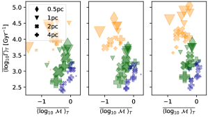
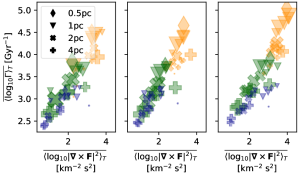
Results from models of isothermal SSDs indicate that highly compressible flows inhibit dynamo activity (Haugen et al., 2004; Federrath et al., 2011, 2014; Seta & Federrath, 2021), while high magnetic Reynolds number Rm makes SSDs more likely and is correlated with higher growth rates (Schekochihin et al., 2002, 2005; Iskakov et al., 2007; Brandenburg, 2011; Schober et al., 2012; Seta et al., 2020; Warnecke et al., 2022).
In Figure 5(a) we display the summary statistics for Mach number against relative growth rate for each bin of volume-averaged magnetic energy growth rate. Overall the expected trend of reducing as increases is visible, more so in the lowest growth rate regions (left panel). We observe that hot gas with high sound speed has low Ms and high relative growth rate and cold gas the inverse. What is, perhaps, unexpected is to see that within each phase there is a trend of increasing with increasing . This can be explained by the counter effect of increased velocities, which drive higher Mach numbers for a given sound speed, but also higher Rm. So increased with should have complementary trends in Rm.
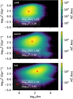
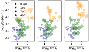
In this highly compressible system it is challenging to calculate Rm as would conventionally be defined for weakly compressible simulations. Instead, we use the ratio of advective to diffusive terms given by Eq. (9). With strongly fluctuating characteristic velocities and length scales applying between the continuously shifting phases, and the very sporadic and flexible scale of the SN forcing, Rm varies as a function of position and time. An illustration of the extent to which Rm varies is shown in the histograms of Figure 6. While the mean Rm is quite modest of order 16 and 45 in the cold and warm phases, there are regions in all phases where Rm , and in the hot phase Rm . For the summary statistics the log mean values are quite informative to identify the trends in SSD dependencies across simulations over time and between phases.
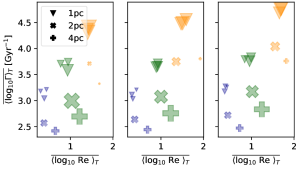
Results for Rm versus are shown in Figure 5(b). Velocities increase with temperature, increasing Rm and supporting faster SSD, an overall trend as would be expected for . Within each phase and within each bin, however, is weakly anticorrelated with Rm, and across each bin the patterns are largely unaffected for cold and warm gas, suggesting higher velocities may be associated with higher Mach numbers. Results are similar for Re versus as shown in Figure 5(c) for samples from models that include explicit viscosity . The higher resolution models () show a good correlation between Re and growth rate. The lower normalization of that correlation seen in the lower resolution models may well be due to reduced kinetic energy from excess cooling in under-resolved density gradients. The comparison between the 1 pc and 0.5 pc models without viscosity suggests that the 1 pc model is well converged. For the hot gas Rm, Re, and all increase for the upper growth rate bin, suggesting increased velocities are associated with rotational rather than compressive flows.
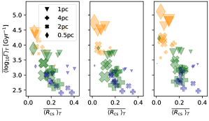
If this were the case, we would expect to see this reflected in the structure of the flow, which we consider in Figure 7 (see analysis of hydrodynamic flow by Käpylä et al., 2018). We use a Helmholtz decomposition to separate the velocity field into purely solenoidal and compressive flows , in which and are, respectively, a vector potential and scalar potential pair from which orthogonal flows and can be derived.
Both flows appear strongly correlated with , although not as clearly as vorticity in Figure 4(a). It is reasonable to expect that the magnitude of compressive and solenoidal flows would be correlated, and as such some common correlation to would be evident. The clearer correlations for (b) rotational rather than (a) compressive flows indicates that the latter is coincidental. Growth rate trends in the warm and cold gas do not alter significantly between bins of even as flow strength varies. In the hot gas clearly increases when increases between low (left) and high (right) bins, especially for high resolution models.
In Figure 7(c) the summary statistics are plotted of the compressive ratio (Kritsuk et al., 2007) defined by
| (11) |
This shows that the ratio of solenoidal energy to total compressive and solenoidal energy is typically between 60% (cold) and 90% (hot). At higher resolution the fraction of energy in solenoidal flow is higher. The compressive ratio reduces from cold to hot phases. The growth rate is directly correlated with the fraction of solenoidal energy.
3.3 Prandtl number variability
The multiphase structure and intermittent forcing of the ISM causes the fluid Reynolds number Re to vary just as was shown for Rm in Figure 6. This results in a wide variation of magnetic Prandtl number Pm. In Gent et al. (2021, see Figures 5[b1] and [b2]) we examined the role of Pm on the SSD in ISM simulations, by varying both viscosity and resistivity . For a fixed , the SSD did not depend on Pm and the energy at which the dynamo saturated was consistently around 5% of equipartition. For a fixed , on the other hand, SSD growth rate did increase with Pm for in the parameter space considered. The energy at saturation increased with Pm, remaining steady for . This suggested that it is the ratio of the Lorentz force to Rm rather than Pm that is the controlling parameter (see also Oishi & Mac Low, 2011, for a similar suggestion in magnetorotational dynamos).
Therefore, here we vary Pm by varying only . Where the viscosity, , and the resistivity, , are explicitly defined, we can nominally express the magnetic Prandtl number, , which is what we shall use here. Alternatively, as a function of position Pm can also vary due to the flows and length scales characteristic at different regions and times altering the effective ratios of Rm to Re. In the Appendix we determine the effective magnetic Prandtl number in various models to examine the relevance the explicit diffusivities to the dynamics (see Figure 12).
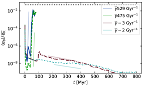
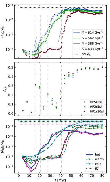
In Figure 8(a) we show the volume averaged magnetic energy density for models with with resolution . Around there is a burst of SSD, common to all three runs, highlighted between the two leftmost vertical dotted lines. Growth rates applying for depend on Pm in this range. Sensitivity to Pm reduces as Pm approaches 5, consistent with the idea that growth rates become asymptotic for higher Pm. We also fit for at , where the growth rate exceeds that for earlier. Under most circumstances we would expect to be lower for the larger , but during this period the fractional volume of the hot gas is higher (Figure 8(b)) in all models than during the earlier subinterval. A surge aligned to the rightmost vertical dotted line is also evident in the high Pm models, although it is inhibited in those by the onset of saturation.
The critical Rm above which SSD can be excited and the typical scaling relations with Rm for the rate of magnetic energy growth are not well determined. For SSD actually decays during two periods, before its final surge. This could be due to Rm varying or changing conditions resulting in a lower critical Rm.
We plot the hot gas fractional volumes for the models with in Figure 8(b). At first, the hot gas fractions for all models coincide. Despite the initial weakness of magnetic effects, the fractional volumes diverge slightly within 20 megayears. The resistive timestep differs between the models; small changes in timestep lead to the chaotic solutions adopting alternate trajectories. For example a delay of a few decades in scheduling a single SN, even at the identical location, alters the specific ambient conditions modifying the remnant evolution and subsequent dynamics, propagating into diverging trajectories between models.
Nevertheless the trends are consistent between models. In the subinterval between the two leftmost vertical dotted lines, is enhanced, corresponding to a burst in SSD activity. The dip in between the middle two vertical lines corresponds to decay in the model and slower growth at higher Pm, followed by another SSD burst aligned with the third vertical line and a peak in , least so for . The value of then rises again at 40 megayears, particularly for , with an accompanying boost in SSD. The described behavior supports the hypothesis that higher SSD activity is correlated with increasing fractional volume of the hot gas .
3.4 Growth trends by phase
To examine our hypothesis further, we split the evolution of the magnetic energy between phases and plot these in Figure 8(c) for the models with and 5. These are normalised by . Horizontal dotted lines of matching color for each phase indicate the time-averaged kinetic energy density by phase . These lines, plotted for , are very similar for .
Usually is smallest in the hot gas, but during the SSD activity bursts, its growth is the most rapid and its energy density then exceeds that of the other two phases. The saturation energy of the hot gas is similar for both models, around at 40 megayears for , and 55 megayears for . In contrast the saturation energy in the cold and warm phases is affected by . In the nonlinear phase the magnetic energy in the hot phase decays to around , while the magnetic energy in the cold phase grows, above in the case of .
Is the latter consistent with compression in the statistical steady MHD state? Under compression, magnetic field strength relates to density , where for compression along field lines up to disc or slab-like compression (Tritsis et al., 2015). In Figure 9, for the two models in Figure 8(c) we plot the mean gas number density in the cold gas (left axis) and the root mean square strength of the magnetic field normalised by cold gas density (right axis), taking . In the interval the dynamo has clearly saturated for the warm and hot gas (Figure 8). If the continued growth of the magnetic field in the cold gas were due to compression of the field with the gas, then we would expect the ratio of to remain steady or even decay. Instead, in both models this ratio continues to increase until , indicating that dynamo remains active in the cold phase. The increasing mean density in the cold gas toward the end of the simulation reflects the increasing fractional volume of hot gas and mean thermal energy density. The cooling in the hot gas is too inefficient to balance the supply of thermal energy from subsequent SNe in the closed system, and thermal runaway will eventually result. Applying in the analysis does not qualitatively alter the development of .
3.5 Supernova rate
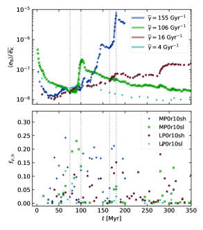
The strength of the SSD in SN-driven turbulence has been found to be sensitive to the SN rate, (Balsara et al., 2004; Gent et al., 2021). Balsara et al. (2004) used an SN rate of . Because of their confinement within the periodic boundaries, these models were dominated by thermal runaway, as described by Kim & Ostriker (2015), in which the fractional volume of hot gas reaches . Therefore, SSD has a steady exponential growth, because the ISM has effectively become a homogeneous, single phase medium. Indeed, in similar experiments by Gent et al. (2021), thermal runaway was easily excited at high resolution () even with . At low resolution (), with consequentially higher numerical diffusion, and thus unphysically strong cooling, thermal runaway was still excited for . Rapid steady acceleration of the SSD occurs, which is excluded here with lower .
In Figure 10(a) we compare evolution of for and at and 4 pc, and (b) the fractional volume of the hot gas . The higher rate produces more hot gas and sustains the dynamo, more so for (blue) than (brown). For lower , decays, but growth occurs briefly in the subinterval between the first two vertical lines, while increases, particularly for (green). Least-squares fits for are shown for this subinterval (green and cyan). Higher occurs for higher with fits for (blue and red) indicated in the second subinterval. Another boost in SSD occurs for after 270 megayears when is at an even higher peak. In general for there is less hot gas than for at each given SN rate, because of higher numerical diffusion and cooling.
Mean kinetic energy density is not strongly affected by the SN rate (Gent et al., 2021, see their Figure 3[d]), so the change in SSD growth rate would appear to be due to the increased heating of the ISM at higher . Figure 10 demonstrates that this is indeed the case. High SSD growth rate coincides with high for hot gas within each model and between models, higher occurs in models that support higher .
3.6 Stratification
Anticipating future examination of the LSD, in Model LP5r8sm-S we consider how stratification affects the SSD. To exclude the LSD, we omit large-scale rotation and shear. Inhomogeneities due to non-periodic boundaries vertically might still cause an LSD effect, so any residual mean magnetic field volume and horizontal component average is subtracted at each timestep. In contrast to the periodic domains, the open vertical boundary enables gas flow and magnetic helicity flux to and from the disk.
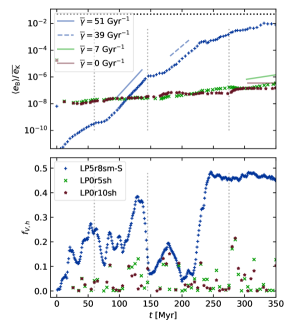
In Figure 11(a) we plot for this model with alongside models with . Given that always increases with in otherwise equivalent models, it is evident that the substantially increased growth rate in model LP5r8sm-S is due to its stratification. We also see from Figure 11(b) that the stratified Model LP5r8sm-S has the largest fractional volume of hot gas, although none of the low resolution periodic models have large (see also Figure 10]b]).
From the summary statistics in Figure 4(b), we find for that the absolute growth of magnetic energy is fastest in the cold gas, but occurs mostly in the warm gas due to its higher fractional volume. In contrast the stratification supports high and high for the hot gas, depicted in Figures 4–7 by a large orange plus symbol.
As increases, the absolute growth rate in the hot gas reduces, as shown in Figure 4(b) (left to right), for , While for it increases. In the cold gas increases for and reduces for higher resolution. At , however, does not vary over time as much as for higher resolution. At all stages in the warm gas is five to ten times larger in the stratified model than the periodic models.
Vorticity in all phases is much lower (Figure 4) at , but of these it is highest in the stratified model. The values of , , and velocities (Figs. 5 and 7), are also highest in the stratified model. Higher velocities, and vorticity, in all phases are possible with stratification, because the gas can expand into lower pressure diffuse gas away from the midplane.
4 Discussion and conclusions
4.1 Differences with isothermal dynamo
Consensus based on studies of isothermal MHD turbulence predicts that , the critical Rm above which SSD can be excited, reduces as Pm increases above with an asymptotic limit of order for (Schekochihin et al., 2002; Schober et al., 2012; Seta et al., 2020). Less directly relevant to our context of ISM turbulence, for low Pm there is a range where has a maximum (Schekochihin et al., 2005; Iskakov et al., 2007; Brandenburg, 2011), and then for again begins to drop (Warnecke et al., 2022). Once excited, the rate of growth of SSD also increases, up to some asymptote, for higher Pm. In these isothermal systems, it has also been demonstrated that as increases it becomes more difficult to excite SSD ( for Haugen et al., 2004) and growth rates are correspondingly reduced (Federrath et al., 2011, 2014). Hence, according to these findings, SSD can be excited in our models, as this threshold value is easily exceeded.
Superficially, these conclusions might appear irrelevant to an SSD in multiphase SN-driven turbulence with respect to the averages across all phases. The response of models with respect to Pm is inconsistent. Higher SN rates with correspondingly higher compressive forcing appear to excite SSD more easily and with larger growth rate. SSD does not appear to follow a dominant eigenmode, establishing a distinct exponential amplification until saturation.
However, detailed analysis reveals that what is inconsistent in this more realistic ISM is the distribution of temperatures, gas densities, and flow properties throughout the thermal phases and over time. Determination of Pm, Rm, Re, and must be specific to each region of the ISM. It is likely that the variation we see by position in these properties occurs also in isothermal simulations, but that the statistics of these remain quite consistent throughout the domain and duration. In a multiphase system, on the other hand, these statistics vary by orders of magnitude as a function of position and time.
The breakdown of the models by phase and overall SSD growth rate shows that the insights from isothermal SSD experiments do apply, but contrary trends, such as increasing growth in SSD with increasing , seen in Figure 5(a), are due to the SSD supportive counter trends, such as increasing velocity (with ). The expected effect of on growth rate is well demonstrated in the anticorrelation going from hot to cold phase. Conversely, in Figure 5(b), Rm seems anticorrelated with SSD growth rate in the hot phase, indicating that SSD is more easily excited as the hot filling fraction and typical temperature of the hot gas increase, even for lower Rm. The expected trend of positive correlation between Rm and SSD growth rate is evident in the differences between phases.
4.2 Growth rates and strength of SSD
In their two-phase simulations, Seta & Federrath (2022) determined that the magnetic energy in their models grows more slowly than in isothermal models with the same forcing and equivalent mean Mach numbers for the warm gas and 5 for the cold gas. Their SSD saturates after around 400 megayears for solenoidal forcing and 800 megayears for compressive forcing, for a grid resolution comparable to Model UP0r10sl. For this and all our 1 pc resolution periodic models, the SSD saturates within 40–60 megayears with mean , 0.6 and 0.25 in the cold, warm and hot gas, respectively. However, in all phases spans around two orders of magnitude over a large proportion of the volume, and outliers extend even further. The variance is much larger than in the two-phase simulations. The faster SSD in our models may, therefore, be less sensitive to the mean , as growth occurs predominantly in low Mach number, high vorticity regions, particularly in the hot gas.
The SSD persists longest in the cold phase and next longest in the warm phase (Fig. 8[c]). We speculate that an explanation for the growth rates differing between phases in three-phase and not in two-phase simulations is that high vorticity generated in the hot gas transfers to warm then cold regions, but with a time delay that is significantly longer than from the warm to cold phase. As a result, we find faster growth in all phases.
Estimates for the post inflationary seed magnetic field are in the range –G (Grasso & Rubinstein, 2001; Subramanian, 2016). With an exponent of this could be amplified to sub-equipartition saturation of around G within 170 to 590 Myr. Given these results consistently yield saturation of the SSD significantly below equipartition with the kinetic energy density (see also Schober et al., 2015), this does not exclude LSD action being sufficient to amplify even the lowest estimates of post-inflation magnetic field to the values observed in high redshift galaxies.
4.3 Interpretation of Rm
It is perhaps surprising, and inconsistent with current understanding of dynamo, to see in Figure 6 locations with , well below isothermal predictions of , coincident with growth rate in cold gas. These are outliers in a highly inhomogeneous multiphase structure, in which there is phase mixing and energy transfer within and between phases. The bulk of the simulation data corresponds to high Rm and high with the positive correlation reflected in the increasing log mean from the cold to hot phase.
To examine whether the high apparent growth rates at low Rm can be explained without SSD, let us approximate the effect of a blast wave following Sedov-Taylor (Sedov, 1959; Taylor, 1950) travelling at , as would occur in an SN remnant with radius near 30 pc in a K medium of uniform gas number density . From Equation (8) with the normalized quantity we can write
| (12) | ||||
Considering the first term with a shock front traveling at into warm gas with sound speed around resolved in our model over three cells, . If the local magnetic field is even twice the volume averaged strength, this would yield . The effect of the other terms and nonadiabatic cooling would adjust this estimate up or down, but nevertheless it remains entirely consistent with the rare high values of and in regions of low Rm in Figure 6.
For a magnetic field perpendicular to the blast wave
| (13) |
reaching a maximum at the shock centre, where the first derivative approaches infinity and the second derivative vanishes, but near zero either side of the shock where the inverse is true. Both can coexist with the compression estimated above, explaining these low Rm outliers in the joint histograms.
Conventionally, a single characteristic Rm for a domain is related to , associated with the single exponential growth rate of the dominant eigenmode of the SSD. The analysis of Grete et al. (2017) found that the Lorentz forces could induce weak nonlocal energy transfers, but that magnetic and kinetic energy transfers in both directions are predominantly highly localised in -space, including for isothermal compressible MHD. Hence, the differences in characteristic length scales between the phases would tend to yield Rm supportive of very different dominant dynamo modes. Thus, in the multiphase ISM the SSD growth rate represents a superposition of varying dynamo modes, in which the dominant modes can switch from one phase to another over time due to heating, cooling and phase mixing.
The mean of the instantaneous localised growth rates collected while is highest have similar magnitude to as fitted in each simulation, supporting the concept of a superposition. Sufficiently high mean or correlated with a supercritical mean Rm would dominate the overall growth rates irrespective of the outliers.
4.4 SSD dependence on vorticity
We considered the properties in the simulations of velocity, Mach number, fluid and magnetic Reynolds numbers, Prandtl number, kinetic and magnetic helicity, and kinetic energy to identify how they relate to the relative and absolute growth rates of magnetic energy and . By far the clearest correlation to growth rate was in the enstrophy, or norm squared vorticity.
The dependence of growth rate on velocity shows a weaker dependence, which is very similar to that of the Helmholtz decomposed flow displayed in Figure 7, and even less correlation is seen in the kinetic energy density. The latter indicates that it is the magnitude of the flow rather than the kinetic energy density that is important to the SSD efficiency.
We break down the statistics into epochs of various rates of volume averaged growth . Periods of higher have higher velocities and vorticity. From the stronger correlation between vorticity and growth, we conclude that the vorticity of the flow drives the SSD. Despite the compressive structure of the SN forcing there is, as expected, a high fraction of rotational flow present, as identified from the Helmholtz decomposition. The excess of rotational to compressive flow is indicated by the compressive ratio at less than 40% and even below 10% in the hot gas. The efficiency of vortex generation is primarily driven in the ISM by the strong baroclinicity, the cross of orthogonal gradients of pressure and density, at the SN shock interactions (see Käpylä et al., 2018). Typically the magnitude of the velocity and the proportion of enstrophy increase with temperature. Fitting data from Figure 4(a) and for the high resolution data only from Figure 7(c), we find that the local growth rate and .
A concern might exist that vorticity could be artificially generated, as has been identified at the intersection of adaptive grids of mixed mesh refinement (Plewa & Müller, 2001), or due to the use of locally varying diffusive schemes (Robertson et al., 2010) at lower resolution. Diffusivity is independent of position in our models, except for its use in resolving shocks. Inspection of the energy spectra (as in Gent et al., 2021, and here in Figure 12 of the Appendix) confirms in all cases that energy peaks are far from the Nyquist frequency and with very low energy near theses scales. Hence, any transfer of energy from the flow to the magnetic field must occur at length scales independent of the shock resolution over a few cells.
The study of vortex generation by Käpylä et al. (2018) was a purely hydrodynamical study, although stratified, with similar levels of vortex generation. It had no hyperdiffusion. Given the relatively low magnetic energy here, even after saturation of the SSD, we can also exclude the generation of vorticity being due to the magnetic field.
4.5 SSD dependence on temperature
We have shown that SSD activity increases when the fractional volume of the hot gas increases, and we have shown that the magnetic energy density in the hot gas grows the most rapidly during these epochs. At other times, though, the magnetic field does not grow as quickly in the hot gas as in the warm gas. The vorticity in the hot gas is also particularly high during these rapid bursts of SSD. So, both the volume and the stirring of the hot gas increase, combining to drive strong dynamo action for a limited period.
In Kirchschlager et al. (2022), we use model UP0r10sl to examine dust-processing due to SN blast waves. The progress of individual remnants are followed in detail for isolated explosions in a dense turbulent region or a diffuse turbulent region. The effects on the magnetic field inside each remnant is instructive for the understanding of SSD in hot gas (see their Figure 1). In the case of the explosion in a dense region, the magnetic field is evacuated from within the remnant and is swept along by the the blast wave for up to 1 megayear. In the case of the diffuse region, the surrounding regions of strong magnetic field are pushed away by the blast wave, but inside the remnant the magnetic field grows, with the interior field strength orders of magnitude stronger at 1 megayear than at the time of the explosion. The SSD is enhanced in the hot gas where the interaction of the blast wave with the inhomogeneous density structure excites strong, interacting reverse shocks that can persist to late times in the diffuse medium. In dense regions, on the other hand, the reverse shocks from the ambient ISM are weak relative to the blast wave and then quickly slow in the relatively high gas density remnant interior.
This is consistent with our finding that the SSD is more sensitive to the vorticity than the kinetic energy, as the diffuse remnant contains relatively low kinetic energy. In our stratified model LP5r8sm-S the SSD is more active, with the ISM typically more diffuse. The SSD accelerates when the hot gas develops more solenoidal turbulence through SN remnant interactions and mergers (such as emerging superbubbles in the local and nearby galactic disks Bik et al., 2018; Sofue & Kataoka, 2021). Simulated superbubbles with magnetic fields (e.g., Ferrière et al., 1991; Stil et al., 2009) have tended to apply uniform ambient fields and smooth ambient gas, such that amplification of the magnetic fields are concentrated around the outer shell due to compression, as in the case of the dense region. Superbubbles in turbulent MHD have been modelled (e.g., Korpi et al., 1999; de Avillez & Breitschwerdt, 2005; Breitschwerdt & de Avillez, 2006; Gressel et al., 2008; Gent et al., 2013a, b), but the local structure of the magnetic field not analysed in such detail.
4.6 Summary of results
We conclude that the SSD in the SN-driven multiphase turbulence of the ISM:
-
a.
has an average growth rate linearly correlated with the average vorticity of the flow, which is efficiently generated by baroclinic effects due to SN blast wave interactions;
-
b.
correspondingly has an average growth rate well correlated with the average magnitude of the rotational flow velocity, as well as the compressible and total velocities and the fluid Reynolds number, and anticorrelates with the compressive ratio;
-
c.
grows as a superposition of varying dynamo modes in each phase and within different regions of each phase;
-
d.
grows intermittently, predominantly during periods when the hot gas, with low sonic Mach number , has strong enstrophy and large volume filling fraction;
-
e.
is thus most efficient in hot gas produced when supernovae explode in diffuse regions, where interacting reverse shocks can have high velocities;
-
f.
is more efficient in a stratified disk, where diffuse gas away from the disk is more easily heated and supports high velocities with low ;
-
g.
and already appears to approach asymptotic solutions at values of , and significantly below the actual values estimated to apply in the ISM, although higher resolution will be required to confirm this point (see Appendix).
Prior to the onset of SSD the magnetic field strength aligns with the gas density, consistent with turbulent mixing, and following saturation of the SSD the field redistributes back into alignment with the gas concentration. The hot gas saturates significantly below equipartition, and even below the the ISM average of around 5% of equipartition with kinetic energy density, while the cold gas saturates at close to the equipartition energy.
References
- Achikanath Chirakkara et al. (2021) Achikanath Chirakkara, R., Federrath, C., Trivedi, P., & Banerjee, R. 2021, Phys. Rev. Lett., 126, 091103, doi: 10.1103/PhysRevLett.126.091103
- Balsara et al. (2004) Balsara, D. S., Kim, J., Mac Low, M.-M., & Mathews, G. J. 2004, ApJ, 617, 339, doi: 10.1086/425297
- Beck (2016) Beck, R. 2016, A&A Rev., 24, 4, doi: 10.1007/s00159-015-0084-4
- Beck et al. (1996) Beck, R., Brandenburg, A., Moss, D., Shukurov, A., & Sokoloff, D. 1996, ARA&A, 34, 155, doi: 10.1146/annurev.astro.34.1.155
- Beck et al. (2003) Beck, R., Shukurov, A., Sokoloff, D., & Wielebinski, R. 2003, A&A, 411, 99, doi: 10.1051/0004-6361:20031101
- Bhat et al. (2016) Bhat, P., Subramanian, K., & Brandenburg, A. 2016, MNRAS, 461, 240, doi: 10.1093/mnras/stw1257
- Bik et al. (2018) Bik, A., Östlin, G., Menacho, V., et al. 2018, A&A, 619, A131, doi: 10.1051/0004-6361/201833916
- Brandenburg (2011) Brandenburg, A. 2011, ApJ, 741, 92, doi: 10.1088/0004-637X/741/2/92
- Brandenburg & Dobler (2002) Brandenburg, A., & Dobler, W. 2002, Computer Physics Communications, 147, 471
- Brandenburg et al. (2007) Brandenburg, A., Korpi, M. J., & Mee, A. J. 2007, ApJ, 654, 945, doi: 10.1086/509143
- Brandenburg & Sarson (2002) Brandenburg, A., & Sarson, G. R. 2002, Phys. Rev. Lett., 88, 055003, doi: 10.1103/PhysRevLett.88.055003
- Brandenburg et al. (2020) Brandenburg, A., Johansen, A., Bourdin, P. A., et al. 2020, arXiv e-prints, arXiv:2009.08231
- Breitschwerdt & de Avillez (2006) Breitschwerdt, D., & de Avillez, M. A. 2006, A&A, 452, L1, doi: 10.1051/0004-6361:20064989
- Chandrasekhar & Fermi (1953) Chandrasekhar, S., & Fermi, E. 1953, ApJ, 118, 116, doi: 10.1086/145732
- Crutcher et al. (2003) Crutcher, R., Heiles, C., & Troland, T. 2003, in Lecture Notes in Physics, Berlin Springer Verlag, Vol. 614, Turbulence and Magnetic Fields in Astrophysics, ed. E. Falgarone & T. Passot, 155–181
- de Avillez & Breitschwerdt (2005) de Avillez, M. A., & Breitschwerdt, D. 2005, A&A, 436, 585, doi: 10.1051/0004-6361:20042146
- de Avillez & Breitschwerdt (2007) —. 2007, ApJ, 665, L35, doi: 10.1086/521222
- Evirgen et al. (2019) Evirgen, C. C., Gent, F. A., Shukurov, A., Fletcher, A., & Bushby, P. J. 2019, MNRAS, 488, 5065, doi: 10.1093/mnras/stz2084
- Federrath et al. (2011) Federrath, C., Chabrier, G., Schober, J., et al. 2011, Phys. Rev. Lett., 107, 114504, doi: 10.1103/PhysRevLett.107.114504
- Federrath & Klessen (2012) Federrath, C., & Klessen, R. S. 2012, ApJ, 761, 156, doi: 10.1088/0004-637X/761/2/156
- Federrath et al. (2014) Federrath, C., Schober, J., Bovino, S., & Schleicher, D. R. G. 2014, ApJ, 797, L19, doi: 10.1088/2041-8205/797/2/L19
- Ferrière (2001) Ferrière, K. M. 2001, Reviews of Modern Physics, 73, 1031, doi: 10.1103/RevModPhys.73.1031
- Ferrière et al. (1991) Ferrière, K. M., Mac Low, M.-M., & Zweibel, E. G. 1991, ApJ, 375, 239, doi: 10.1086/170185
- Field et al. (1969) Field, G. B., Goldsmith, D. W., & Habing, H. J. 1969, ApJ, 155, L149, doi: 10.1086/180324
- Fletcher et al. (2011) Fletcher, A., Beck, R., Shukurov, A., Berkhuijsen, E. M., & Horellou, C. 2011, MNRAS, 412, 2396, doi: 10.1111/j.1365-2966.2010.18065.x
- Fryxell et al. (1991) Fryxell, B., Mueller, E., & Arnett, D. 1991, ApJ, 367, 619, doi: 10.1086/169657
- Gent (2012) Gent, F. A. 2012, PhD thesis, Newcastle University School of Mathematics and Statistics
- Gent et al. (2020) Gent, F. A., Mac Low, M.-M., Käpylä, M. J., Sarson, G. R., & Hollins, J. F. 2020, Geophysical and Astrophysical Fluid Dynamics, 114, 77, doi: 10.1080/03091929.2019.1634705
- Gent et al. (2021) Gent, F. A., Mac Low, M.-M., Käpylä, M. J., & Singh, N. K. 2021, ApJ, 910, L15, doi: 10.3847/2041-8213/abed59
- Gent et al. (2013a) Gent, F. A., Shukurov, A., Fletcher, A., Sarson, G. R., & Mantere, M. J. 2013a, MNRAS, 432, 1396, doi: 10.1093/mnras/stt560
- Gent et al. (2013b) Gent, F. A., Shukurov, A., Sarson, G. R., Fletcher, A., & Mantere, M. J. 2013b, MNRAS, 430, L40, doi: 10.1093/mnrasl/sls042
- Grasso & Rubinstein (2001) Grasso, D., & Rubinstein, H. R. 2001, Phys. Rep., 348, 163, doi: 10.1016/S0370-1573(00)00110-1
- Gressel et al. (2008) Gressel, O., Elstner, D., Ziegler, U., & Rüdiger, G. 2008, A&A, 486, L35, doi: 10.1051/0004-6361:200810195
- Grete et al. (2017) Grete, P., O’Shea, B. W., Beckwith, K., Schmidt, W., & Christlieb, A. 2017, Physics of Plasmas, 24, 092311, doi: 10.1063/1.4990613
- Hanasz et al. (2009) Hanasz, M., Wóltański, D., & Kowalik, K. 2009, ApJ, 706, L155, doi: 10.1088/0004-637X/706/1/L155
- Harnett et al. (2004) Harnett, J., Ehle, M., Fletcher, A., et al. 2004, A&A, 421, 571, doi: 10.1051/0004-6361:20034377
- Haugen & Brandenburg (2004) Haugen, N. E. L., & Brandenburg, A. 2004, Phys. Rev. E, 70, 036408, doi: 10.1103/PhysRevE.70.036408
- Haugen et al. (2004) Haugen, N. E. L., Brandenburg, A., & Mee, A. J. 2004, MNRAS, 353, 947, doi: 10.1111/j.1365-2966.2004.08127.x
- Hill et al. (2018) Hill, A. S., Mac Low, M.-M., Gatto, A., & Ibáñez-Mejía, J. C. 2018, ApJ, 862, 55, doi: 10.3847/1538-4357/aacce2
- Hollins et al. (2017) Hollins, J. F., Sarson, G. R., Shukurov, A., Fletcher, A., & Gent, F. A. 2017, ApJ, 850, 4, doi: 10.3847/1538-4357/aa93e7
- Iskakov et al. (2007) Iskakov, A. B., Schekochihin, A. A., Cowley, S. C., McWilliams, J. C., & Proctor, M. R. E. 2007, Phys. Rev. Lett., 98, 208501, doi: 10.1103/PhysRevLett.98.208501
- Joung & Mac Low (2006) Joung, M. K. R., & Mac Low, M.-M. 2006, ApJ, 653, 1266
- Joung et al. (2009) Joung, M. R., Mac Low, M.-M., & Bryan, G. L. 2009, ApJ, 704, 137, doi: 10.1088/0004-637X/704/1/137
- Käpylä et al. (2018) Käpylä, M. J., Gent, F. A., Väisälä, M. S., & Sarson, G. R. 2018, A&A, 611, A15, doi: 10.1051/0004-6361/201731228
- Karak & Brandenburg (2016) Karak, B. B., & Brandenburg, A. 2016, ApJ, 816, 28, doi: 10.3847/0004-637X/816/1/28
- Kim & Ostriker (2015) Kim, C.-G., & Ostriker, E. C. 2015, ApJ, 802, 99, doi: 10.1088/0004-637X/802/2/99
- Kirchschlager et al. (2022) Kirchschlager, F., Mattsson, L., & Gent, F. A. 2022, in preparation
- Korpi et al. (1999) Korpi, M. J., Brandenburg, A., Shukurov, A., & Tuominen, I. 1999, A&A, 350, 230
- Kritsuk et al. (2007) Kritsuk, A. G., Norman, M. L., Padoan, P., & Wagner, R. 2007, ApJ, 665, 416, doi: 10.1086/519443
- Mac Low & Klessen (2004) Mac Low, M.-M., & Klessen, R. S. 2004, Reviews of Modern Physics, 76, 125, doi: 10.1103/RevModPhys.76.125
- McCourt et al. (2012) McCourt, M., Sharma, P., Quataert, E., & Parrish, I. J. 2012, MNRAS, 419, 3319, doi: 10.1111/j.1365-2966.2011.19972.x
- McKee & Ostriker (1977) McKee, C. F., & Ostriker, J. P. 1977, ApJ, 218, 148, doi: 10.1086/155667
- Oishi & Mac Low (2011) Oishi, J. S., & Mac Low, M.-M. 2011, ApJ, 740, 18
- Plewa & Müller (2001) Plewa, T., & Müller, E. 2001, Computer Physics Communications, 138, 101, doi: 10.1016/S0010-4655(01)00199-0
- Rieder & Teyssier (2016) Rieder, M., & Teyssier, R. 2016, MNRAS, 457, 1722, doi: 10.1093/mnras/stv2985
- Robertson et al. (2010) Robertson, B. E., Kravtsov, A. V., Gnedin, N. Y., Abel, T., & Rudd, D. H. 2010, MNRAS, 401, 2463, doi: 10.1111/j.1365-2966.2009.15823.x
- Rogachevskii & Kleeorin (2007) Rogachevskii, I., & Kleeorin, N. 2007, Phys. Rev. E, 76, 056307, doi: 10.1103/PhysRevE.76.056307
- Sánchez-Salcedo et al. (2002) Sánchez-Salcedo, F. J., Vázquez-Semadeni, E., & Gazol, A. 2002, ApJ, 577, 768, doi: 10.1086/342223
- Sarazin & White (1987) Sarazin, C. L., & White, III, R. E. 1987, ApJ, 320, 32, doi: 10.1086/165522
- Schekochihin et al. (2002) Schekochihin, A. A., Boldyrev, S. A., & Kulsrud, R. M. 2002, ApJ, 567, 828, doi: 10.1086/338697
- Schekochihin et al. (2005) Schekochihin, A. A., Haugen, N. E. L., Brandenburg, A., et al. 2005, ApJ, 625, L115, doi: 10.1086/431214
- Schober et al. (2012) Schober, J., Schleicher, D., Federrath, C., Klessen, R., & Banerjee, R. 2012, Phys. Rev. E, 85, 026303, doi: 10.1103/PhysRevE.85.026303
- Schober et al. (2015) Schober, J., Schleicher, D. R. G., Federrath, C., Bovino, S., & Klessen, R. S. 2015, Phys. Rev. E, 92, 023010, doi: 10.1103/PhysRevE.92.023010
- Sedov (1959) Sedov, L. I. 1959, Similarity and Dimensional Methods in Mechanics (New York: Academic Press)
- Seta et al. (2020) Seta, A., Bushby, P. J., Shukurov, A., & Wood, T. S. 2020, Phys. Rev. Fluids, 5, 043702, doi: 10.1103/PhysRevFluids.5.043702
- Seta & Federrath (2021) Seta, A., & Federrath, C. 2021, Physical Review Fluids, 6, 103701, doi: 10.1103/PhysRevFluids.6.103701
- Seta & Federrath (2022) —. 2022, MNRAS, 514, 957, doi: 10.1093/mnras/stac1400
- Sofue & Kataoka (2021) Sofue, Y., & Kataoka, J. 2021, MNRAS, 506, 2170, doi: 10.1093/mnras/stab1857
- Sridharan et al. (2014) Sridharan, T. K., Rao, R., Qiu, K., et al. 2014, ApJ, 783, L31, doi: 10.1088/2041-8205/783/2/L31
- Steinwandel et al. (2019) Steinwandel, U. P., Beck, M. C., Arth, A., et al. 2019, MNRAS, 483, 1008, doi: 10.1093/mnras/sty3083
- Stil et al. (2009) Stil, J., Wityk, N., Ouyed, R., & Taylor, A. R. 2009, The Astrophysical Journal, 701, 330, doi: 10.1088/0004-637x/701/1/330
- Subramanian (2016) Subramanian, K. 2016, Reports on Progress in Physics, 79, 076901, doi: 10.1088/0034-4885/79/7/076901
- Taylor (1950) Taylor, G. 1950, Royal Society of London Proceedings Series A, 201, 159, doi: 10.1098/rspa.1950.0049
- Tritsis et al. (2015) Tritsis, A., Panopoulou, G. V., Mouschovias, T. C., Tassis, K., & Pavlidou, V. 2015, Monthly Notices of the Royal Astronomical Society, 451, 4384, doi: 10.1093/mnras/stv1133
- van Loo et al. (2012) van Loo, S., Hartquist, T. W., & Falle, S. A. E. G. 2012, Astronomy and Geophysics, 53, 5.31, doi: 10.1111/j.1468-4004.2012.53531.x
- Warnecke et al. (2022) Warnecke, J., Käpylä, M. J., Gent, F. A., & Rheinhardt, M. 2022, submitted Nat. Astron., doi: 10.21203/rs.3.rs-1819381/v1
- Wolfire et al. (1995) Wolfire, M. G., Hollenbach, D., McKee, C. F., Tielens, A. G. G. M., & Bakes, E. L. O. 1995, ApJ, 443, 152, doi: 10.1086/175510
Appendix A Effective Prandtl number
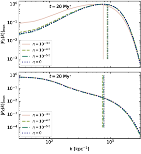
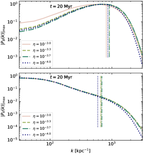
Examples of the magnetic and kinetic energy spectra are displayed in Figure 12 to confirm that the nominal are reflected in the effective magnetic Prandtl number
| (A1) |
in which and are the wavenumbers where the dissipative range begins. At the time indicated, early in the kinematic stage, the spectra are averaged over snapshots spanning and then Gaussian smoothed with . To aid comparison the spectra are all normalised by their maximum.
The wavenumbers and their ratios are listed in Table 4 for each parameter and in the models. These include some models not listed in Table 1, but included in Gent et al. (2021). is determined as the lowest wavenumber after the intertial range for which the log gradient of and for , where the log gradient of . In the case of for , the numerical diffusivities of hyperdiffusion and shock diffusion appear to dominate, with . For this is sufficient to obtain , which should nominally be the case for any .
For we obtain in all cases, due to the higher effective numerical viscosity than resistivity. Nonetheless, the difference between and is sufficient to explain the differences, between the model and . However, we should be cautious about concluding whether the SSD is converging above Pm=5 until we increase resolution or reduce the effective numerical diffusivities.
| 0 | 1e-03 | 785.4 | 760.9 | 0 | 0.97 |
| 0 | 1e-04 | 736.3 | 883.6 | 0 | 1.20 |
| 0 | 1e-05 | 760.9 | 908.1 | 0 | 1.19 |
| 0 | 0e+00 | 785.4 | 908.1 | 1.16 | |
| 1e-3 | 1e-03 | 662.7 | 809.9 | 1 | 1.22 |
| 1e-3 | 5e-04 | 662.7 | 908.1 | 2 | 1.37 |
| 1e-3 | 2e-04 | 687.2 | 908.1 | 5 | 1.32 |
| 1e-3 | 1e-04 | 589.0 | 859.0 | 10 | 1.46 |