The Solvability of Interpretability Evaluation Metrics
Abstract
Feature attribution methods are popular for explaining neural network predictions, and they are often evaluated on metrics such as comprehensiveness and sufficiency. In this paper, we highlight an intriguing property of these metrics: their solvability. Concretely, we can define the problem of optimizing an explanation for a metric, which can be solved by beam search. This observation leads to the obvious yet unaddressed question: why do we use explainers (e.g., LIME) not based on solving the target metric, if the metric value represents explanation quality? We present a series of investigations showing strong performance of this beam search explainer and discuss its broader implication: a definition-evaluation duality of interpretability concepts. We implement the explainer and release the Python solvex package for models of text, image and tabular domains.
1 Introduction
For neural network models deployed in high stakes domains, the explanations for predictions are often as important as the predictions themselves. For example, a skin cancer detection model may work by detecting surgery markers (Winkler et al., 2019) and an explanation that reveals this spurious correlation is highly valuable. However, evaluating the correctness (or faithfulness) of explanations is fundamentally ill-posed: because the explanations are used to help people understand the reasoning of the model, we cannot check it against the ground truth reasoning, as the latter is not available.
As a result, correctness evaluations typically employ certain alternative metrics. For feature attribution explanations, they work under a shared principle: changing an important feature should have a large impact on the model prediction. Thus, the quality of the explanation is defined by different formulations of the model prediction change, resulting in various metrics such as comprehensiveness and sufficiency (DeYoung et al., 2020). To develop new explanation methods (Fig. 1, left), people generally identify a specific notion of feature importance (e.g., local sensitivity), propose the corresponding explainer (e.g., gradient saliency (Simonyan et al., 2013)), evaluate it on one or more metrics, and claim its superiority based on favorable results vs. baseline explainers. We call these explainers heuristic as they are motivated by pre-defined notions of feature importance.
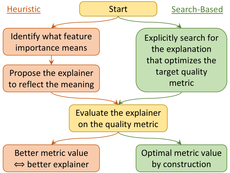
In this paper, we show that all these metrics are solvable, in that we can define an explanation as the one that optimizes a metric value and search for it. The obvious question is then: if we take a specific target metric to represent correctness, why don’t we just search for the metric-optimal explanation (Fig. 1, right) but take the more convoluted route of developing heuristic explanations and then evaluating them (Fig. 1, left)?
There are several possible reasons. First, the optimization problem may be so hard that we cannot find an explanation better than the heuristic ones. The bigger concern, however, is that of Goodhart’s Law. In other words, as soon as a metric is used in explicit optimization, it ceases to be a good metric. Concretely, the explanation may overfit to the particular metric and perform much worse on closely related ones (Chan et al., 2022), or overfit to the model and effectively adversarially attack the model when assigning word importance (Feng et al., 2018). It may also perform poorly on evaluations not based on such metrics, such as ground truth alignment (Zhou et al., 2022a).
We assess these concerns, taking the widely used comprehensiveness and sufficiency metrics (DeYoung et al., 2020) as the optimization target. Our findings, however, largely dispel every concern. A standard beam search produces explanations that greatly outperform existing one such as LIME and SHAP on the target metric. On several other metrics, the search-based explainer also performs favorably on average. There is no strong evidence of it adversarially exploiting the model either, and it achieves competitive performances on a suite of ground truth-based evaluations.
Thus, we advocate for wider adoptions of the explainer, which is domain-general and compatible with models on image and tabular data as well. As an engineering contribution, we release the Python solvex package (solvability-based explanation) and demonstrate its versatility in App.A.
More broadly, the solvability phenomenon is one facet of the definition-evaluation duality, which asserts an equivalence between definitions and evaluations. Solvability recognizes that for each evaluation metric, we can define explainer that performs optimally on this metric. Conversely, for each explainer, we can also come up with an evaluation metric that ranks this explainer on top – a straightforward one would be the negative distance between the explanation under evaluation and the “reference explanation” generated by the explainer.
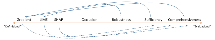
While the community has mostly agreed on a spectrum on which various interpretability concepts (Fig. 2) are located, duality allows every concept to be moved freely on the scale. We explored two particular movements as represented by the solid arrows, but the more general investigation of this operation could be of both theoretical and practical interest. In addition, given that definitions and evaluations are really two sides of the same coin, we need to reflect how to best evaluate explanations. Sec. 6 argues to measure their demonstrable utilities in downstream tasks, and present potential ways and ideas to better align the interpretability research with such goals.
2 Background and Related Work
In this section, we give a concise but unified introduction to the popular feature attribution explainers and evaluation metrics studied in this paper.
2.1 Feature Attribution Explainers
We focus on feature attribution explanations, which explains an input by a vector where represents the “contribution” of to the prediction. Many different definitions for contribution have been proposed and we consider the following five.
- •
-
•
Integrated gradient (IntG) (Sundararajan et al., 2017) is the path integral of the embedding gradient along the line segment from the zero embedding value to the actual value.
-
•
LIME (Ribeiro et al., 2016) is the coefficient of a linear regression in the local neighborhood.
- •
-
•
Occlusion (Occl) (Li et al., 2016b) is the change in prediction when a word is removed from the input while all other words remain.
2.2 Feature Attribution Evaluations
Naturally, different definitions result in different explanation values. As findings (e.g., Adebayo et al., 2018; Nie et al., 2018) suggest that some explanations are not correct (i.e., faithfully reflecting the model’s reasoning process), many evaluations are proposed to quantify the correctness of different explanations. Not having access to the ground truth model working mechanism (which is what explanations seek to reveal in the first place), they are instead guided by one principle: changing an important feature (as judged by the explanation) should have a large impact on the prediction, and the magnitude of the impact is taken as explanation quality. However, there are different ways to quantify the impact, leading to different evaluations, and we consider six in this paper.
Let be a function that we want to explain, such as the probability of the target class. For an input of words, according to an explanation , we can create a sequence of input deletions where is the the input but with most important features removed. Thus, we have and being the empty string.111We define feature removal as the literal deletion of the word from the sentence, which is a popular practice. Other methods replace the token with [UNK], [MASK] or zero embedding, are more sophisticated such as performing BERT mask filling (Kim et al., 2020). While our current approach could lead to out-of-distribution instances, we adopt it due to its popularity. A thorough investigation for the best strategy is orthogonal to our paper and beyond its scope. The comprehensiveness (DeYoung et al., 2020) is defined as
| (1) |
It measures the deviation from the original model prediction when important features (according to ) are successively removed, and therefore a larger value is desirable. It was also proposed for computer vision models as the area over perturbation curve (AoPC) by Samek et al. (2016).
Analogously, we can define the sequence of input insertions , where is the input with the most important features present. Thus, is the empty string and , but otherwise the sequences of input insertions and deletions do not mirror each other. The sufficiency (DeYoung et al., 2020) is defined as
| (2) |
It measures the gap to the original model prediction that remains (i.e., convergence to the model prediction) when features are successively inserted from the most important to the least. Therefore, a smaller value is desirable.
Another interpretation of prediction change just considers decision flips. Let be the function that outputs the most likely class of an input. The decision flip by removing the most important token (Chrysostomou and Aletras, 2021) is defined as
| (3) |
which measures whether removing the most important token changes the decision. Across a dataset, its average value gives the overall decision flip rate, and a higher value is desirable.
The fraction of token removals for decision flip (Serrano and Smith, 2019) is defined as
| (4) |
and we define if no value of leads to the decision flip. This metric represents the fraction of feature removals that is needed to flip the decision, and hence a lower value is desirable.
Last, two metrics evaluate correlations between model prediction and feature importance. For and , we define the sequence of marginal feature deletions such that is original input with only the -th important feature removed. The deletion rank correlation (Alvarez-Melis and Jaakkola, 2018b) is defined as
| (5) | |||
| (6) |
where is the Spearman rank correlation coefficient between the two input vectors. Intuitively, this metric asserts that suppressing a more important feature should have a larger impact to the model prediction. A higher correlation is desirable.
The insertion rank correlation (Luss et al., 2021) is defined as
| (7) | |||
| (8) |
and recall that is the sequence of inputs with increasingly more important features inserted, starting from the empty string to the full input . This metric asserts that the model prediction on this sequence should increase monotonically to the original prediction. Also a higher correlation is desirable.
Related to our proposed notion of solvability is the phenomenon that some metric values seem to favor some explainers (Pham et al., 2022; Ju et al., 2022). While it is often used to argue against the use of certain evaluations, we take this idea to the extreme, which culminates in the solvability property, and find that metric-solving (Def. 3.1) explanations from some metrics can be high-quality.
3 The Solvability of Evaluation Metrics
Now we establish the central observation of this paper: the solvability of these evaluation metrics. Observe that each evaluation metric, e.g., comprehensiveness , is defined on the input and the explanation , and its computation only uses the model prediction function (or derived from for the two decision flip metrics). In addition, the form of feature attribution explanation constrains to be a vector of the same length as , or .
Without loss of generality, we assume that the metrics are defined such that a higher value means a better explanation (e.g., redefining the sufficiency to be the negative of its original form). We formalize the concept of solvability as follows:
Definition 3.1.
For a metric and an input , an explanation solves the metric if for all . We also call the -solving explanation.
Notably, there are already two explanation-solving-metric cases among the ones in Sec. 2.
Theorem 1.
The occlusion explainer solves the DFMIT and RankDel metrics.
The proof follows from the definition of the explainer and the two metrics. Occlusion explainer defines token importance as the prediction change when each the token is individually removed, thus the most important token is the one that induces the largest change, which makes it most likely to flip the decision under DFMIT. In addition, because token importance is defined as the model prediction change, its rank correlation with the latter (i.e., RankDel) is maximal at 1.0.
Thm. 1 highlights an important question: if we take DFMIT or RankDel as the metric (i.e., indicator) of explanation quality, why should we consider any other explanation, when the occlusion explanation provably achieves the optimum? A possible answer is that the metrics themselves are problematic. For example, one can argue that the DFMIT is too restrictive for overdetermined input: when redundant features (e.g., synonyms) are present, removing any individual one cannot change the prediction, such as for the sentiment classification input of “This movie is great, superb and beautiful.”
Nonetheless, the perceived quality of a metric can be loosely inferred from its adoption by the community, and the comprehensiveness and sufficiency metrics (DeYoung et al., 2020) are by far the most widely used. They overcome the issue of DFMIT by also considering inputs with more than one token removed. Since a metric is scalar-valued, we combine comprehensiveness and sufficiency into comp-suff difference , defined as (recall that a lower sufficiency value is better):
| (9) |
Again, we face the same question: if is solvable, why should any heuristic explainers be used instead of the -solving ? In the next two sections, we seek to answer it by first proposing a beam search algorithm to (approximately) find and then explore its various properties.
4 Solving Metrics with Beam Search
We first define two properties that are satisfied by some metrics: value agnosticity and additivity.
Definition 4.1.
For an input with explanation , we define the ranked importance as . In other word, the with is the most important, and that with is the least. A metric is value-agnostic if for all and that induce the same ranked importance, we have
| (10) |
A value-agnostic metric has at most unique values across all possible explanations for an input of length . Thus, in theory, an exhaustive search over the permutations of the list is guaranteed to find the that solves the metric.
Definition 4.2.
A metric is additive if it can be written in the form of
| (11) |
for some function , where reveals the attribution values of most important features according to but keeps the rest inaccessible.
Theorem 2.
Comprehensiveness, sufficiency and their difference are value-agnostic and additive.
The proof is straightforward, by observing that both and can be created from and the ordering of . In fact, all metrics in Sec. 2 are value-agnostic (but only some are additive).
A metric satisfying these two properties admits an efficient beam search algorithm to approximately solve it. As can be considered as a partial explanation that only specifies the top- important features, we start with , and try each feature as most important obtain . With beam size , if there are more than features, we keep the top- according to the partial sum. This extension procedure continues until all features are added, and top extension is then . Alg. 1 documents the procedure, where extends and returns a set of explanations, in which each new one has value on one previously empty entry of . Finally, note that generated on Line 8 has entry values in , but some features may contribute against the prediction (e.g., “This movie is truly innovative although slightly cursory.”). Thus, we post-process by shifting all values by such that the new values (in ) maximally satisfy the sign of marginal contribution of each word (i.e., the sign of the occlusion saliency).
Without the additive property, beam search is not feasible due to the lack of partial metric values. However, Zhou et al. (2021) presented a simulated annealing algorithm (Kirkpatrick et al., 1983) to search for the optimal data acquisition order in active learning, and we can use a similar procedure to search for the optimal feature importance order. If the metric is value-sensitive, assuming differentiability with respect to the explanation value, methods such as gradient descent can be used. Since we focus on comprehensiveness and sufficiency in this paper, the development and evaluation of these approaches are left to future work.
5 Experiments
We investigate various properties of the beam search explainer vs. existing heuristic explainers, using the publicly available textattack/roberta-base-SST-2 model on the SST dataset (Socher et al., 2013) as a case study. The sentiment value for each sentence is a number between 0 (very negative) and 1 (very positive), which we binarize into two classes of and . Sentences with sentiment values in middle are discarded. The average sentence length is 19, making the exhaustive search impossible. We use a beam size of 100 to search for -solving explanation E∗. All reported statistics are computed on the test set.
Fig. 3 presents two explanations, with additional ones in Fig. 11 of App. C. While we need more quantitative analyses (carried out below) for definitive conclusions on its various properties, E∗ explanations at least looks reasonable and is likely to help people understand the model by highlighting the high importance of sentiment-laden words.
A worthy tribute to a great humanitarian and her vibrant ‘ co-stars . ’
So stupid , so ill-conceived , so badly drawn , it created whole new levels of ugly .
5.1 Performance on the Target Metric
We compare E∗ to heuristic explainers on the metric, with results shown in Tab. 5.1 along with the associated and . A random explanation baseline is included for reference. We can see that E∗ achieves the best , often by a large margin. It also tops the ranking separately for and , which suggests that an explanation could be optimally comprehensive and sufficient at the same time.
| Explainer | Comp | Suff | Diff | |
| Grad | 0.327 | 0.108 | 0.218 | |
| IntG | 0.525 | 0.044 | 0.481 | |
| LIME | 0.682 | 0.033 | 0.649 | |
| SHAP | 0.612 | 0.034 | 0.578 | |
| Occl | 0.509 | 0.040 | 0.469 | |
| \cdashline1-4 E∗ | 0.740 | 0.020 | 0.720 | |
| Random | 0.218 | 0.212 | 0.006 | |
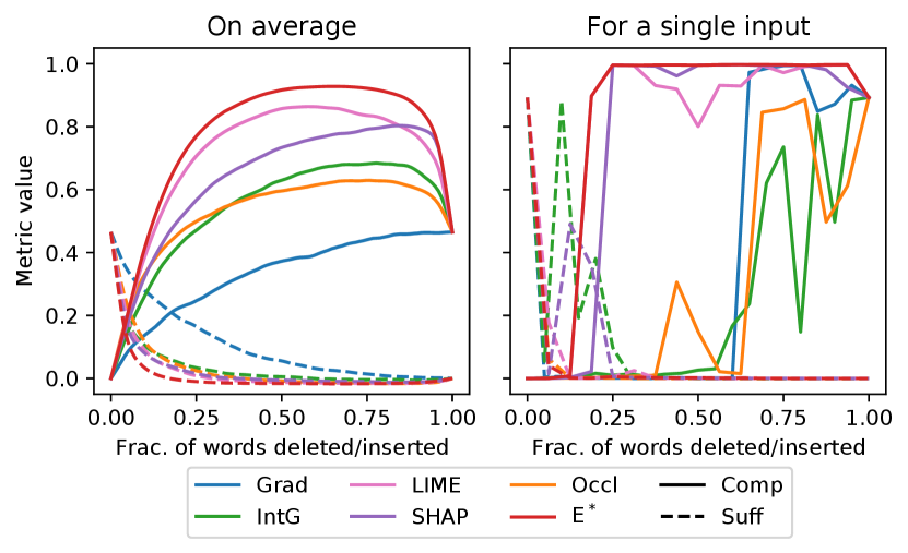
To visually understand how the model prediction changes during feature removal and insertion, we plot in Fig. 4 the values of and (i.e., the summands in Eq. 1 and 2), as a function of . The left panel shows the curves averaged across all test set instances, and the right panel shows those for a specific instance. and are thus the areas under the solid and dashed curves respectively. The curves for E∗ dominate the rest, and, on individual inputs, are also much smoother than those for other explanations.
One concern for beam search is its efficiency, especially compared to those that only require a single pass of the model such as the vanilla gradient. However, we note that explanations, unlike model predictions, are rarely used in real-time decision making. Instead, they are mostly used for debugging and auditing purposes, and incurring a longer generation time to obtain a higher-quality explanation is often beneficial. On a single RTX3080 GPU card without any in-depth code optimization, the metric values and time costs for various beam sizes are presented in Tab. 2, with statistics for the best explainer LIME also listed for comparison.
| 1 | 5 | 10 | 20 | 50 | 100 | LIME | |
| 0.717 | 0.731 | 0.734 | 0.736 | 0.739 | 0.740 | 0.682 | |
| 0.020 | 0.020 | 0.020 | 0.020 | 0.020 | 0.020 | 0.033 | |
| 0.697 | 0.711 | 0.714 | 0.716 | 0.719 | 0.720 | 0.649 | |
| 0.38 | 0.77 | 1.15 | 1.72 | 2.85 | 4.37 | 4.75 |
Expectedly, the metric values increase with increasing beam size, but the improvement is meager after 10 beams. More importantly, beam search is not slow – it is still faster than LIME even with 100 beams, and the single-beam version outperforms LIME by a decent margin while being more than 10 times faster. Thus, these results establish that if we take comprehensiveness and sufficiency as the quality metrics, there is really no reason not to use the beam search explainer directly.
5.2 Performance on Other Metrics
Sec. 2 lists many metrics that all operationalize the same principle that changing important features should have large impact on model prediction, but in different ways. A potential argument against the explicit beam search optimization is the fulfillment of Goodhart’s Law: E∗ overfits to the metric by exploiting its realization (i.e., Eq. 1 and 2) of this principle and not truly reflecting its “spirit.”
To establish the legitimacy of this opposition, we evaluate all the explainers on the remaining four metrics in Sec. 2, and present the results in Tab. 5.2.
| Explainer | DFMIT | DFFrac | RankDel | RankIns | |
| Grad | 10.5% | 54.5% | 0.162 | 0.521 | |
| IntG | 16.9% | 39.6% | 0.369 | 0.468 | |
| LIME | 25.5% | 28.1% | 0.527 | 0.342 | |
| SHAP | 23.0% | 36.1% | 0.369 | 0.458 | |
| Occl | 26.4% | 40.6% | 1.000 | 0.396 | |
| \cdashline1-5 E∗ | 25.0% | 25.2% | 0.438 | 0.423 | |
| Random | 3.4% | 72.3% | 0.004 | 0.599 | |
Since the occlusion explainer solves DFMIT and RankDel (Thm. 1), it ranks the best on these two metrics, as expected. Nonetheless, E∗ still ranks competitively on these two metrics and comes out ahead on DFFrac. The only exception is RankIns, on which the random explanation surprisingly performs the best. We carefully analyze it in App. D and identify a fundamental flaw in this metric.
Last, note that we can also incorporate any of these metrics into the objective function (which already contains two metrics: and ), and search for E∗ that performs overall the best, if so desired. We leave this investigation to future work.
5.3 Explainer “Attacking” the Model
Another concern is that the search procedure may overfit to the model. Specifically, removing a word in a partial sentence drastically changes the model prediction but does not have the same effect for most other . This makes E∗ assign an overly high attribution, as only happens to have a high impact in one particular case. By contrast, explainers like LIME and SHAP automatically avoid this issue by computing the average contribution of on many different partial sentences.
We test this concern by locally perturbing the explanation. If E∗ uses many such “adversarial attacks,” we should expect its metric values to degrade sharply under perturbation, as the high-importance words (according to E∗) will no longer be influential in different partial sentence contexts.
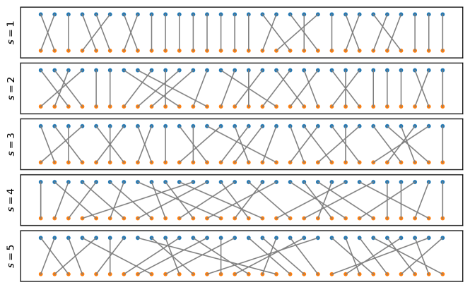
To perturb the explanation, we first convert each explanation to its ranked importance version using in Def. 4.1, which does not affect any metric as they are value-agnostic. Then we define the perturbed rank by adding to each entry of an independent Gaussian noise: with . Thus, two words and with have their ordering switched if . A visualization of the switching with different is in Fig. 12 of App. E.
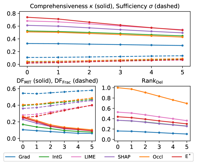
Fig. 5 plots the metrics under different values (RankIns not shown due to its intrinsic issue discussed in App. D). Everything degrades to various extents. Although E∗ degrades slightly faster than the rest on and DFFrac (and on par on others), it still achieves best results even at , with many order switches (Fig. 12), and a faster degradation is reasonable anyway for metrics with better starting values (c.f. occlusion on RankDel).
The evidence suggests that there is at most a slight model overfitting phenomenon, as E∗ remains comparable to other explainers under quite severe perturbation. Furthermore, we can incorporate perturbation robustness into metric solving to obtain an E∗ that degrade less, similar to adversarial training (Madry et al., 2018). We leave the exploration of this idea to future work.
App. F describes another assessment of model overfitting, though with a mild assumption and relying on word-level sentiment scores provided by the SST dataset. Similar conclusions are reached.
5.4 Ground Truth Recovery
| Type | ||
| Short | terrible, awful, disaster, worst, never | excellent, great, fantastic, brilliant, enjoyable |
| Long | A total waste of time. Not worth the money! Is it even a real film? Overall it looks cheap. | I like this movie. This is a great movie! Such a beautiful work. Surely recommend it! |
| Replacement word sets | ||
| a, an, the | a | the |
| in, on, at | in | on |
| I, you | I | you |
| he, she | he | she |
| can, will, may | can | may |
| could, would, might | could | might |
| (all forms of be) | is | are |
| (all punctuation marks) | (period) | (comma) |
| Short Addition | Long Addition | Replacement | |||||||||||
| Sym | Asym | Sym | Asym | Sym | Asym | ||||||||
| Explainer | Pr | NR | Pr | NR | Pr | NR | Pr | NR | Pr | NR | Pr | NR | |
| Grad | 0.91 | 0.06 | 0.51 | 0.08 | 0.70 | 0.37 | 0.77 | 0.30 | 0.50 | 0.75 | 0.51 | 0.74 | |
| IntG | 0.82 | 0.10 | 0.60 | 0.21 | 0.60 | 0.76 | 0.70 | 0.55 | 0.49 | 0.74 | 0.48 | 0.74 | |
| LIME | 1.00 | 0.06 | 1.00 | 0.06 | 0.72 | 0.60 | 0.84 | 0.32 | 0.63 | 0.65 | 0.54 | 0.71 | |
| SHAP | 0.98 | 0.07 | 1.00 | 0.06 | 0.61 | 0.83 | 0.75 | 0.98 | 0.65 | 0.67 | 0.62 | 0.68 | |
| Occl | 1.00 | 0.06 | 1.00 | 0.06 | 0.72 | 0.59 | 0.79 | 0.42 | 0.40 | 0.80 | 0.40 | 0.85 | |
| \cdashline1-13 E∗ | 1.00 | 0.06 | 1.00 | 0.06 | 0.67 | 0.64 | 0.92 | 0.38 | 0.60 | 0.66 | 0.54 | 0.73 | |
| Random | 0.06 | 0.54 | 0.07 | 0.53 | 0.25 | 0.89 | 0.24 | 0.88 | 0.27 | 0.85 | 0.28 | 0.85 | |
For a model trained on a natural dataset, its ground truth working mechanism is rarely available – in fact, arguably the very purpose of interpretability methods is to uncover it. Thus, a series of work (e.g., Zhou et al., 2022a) proposed methods to modify the dataset such that a model trained on the new dataset has to follow a certain working mechanism to achieve high performance, which allows for evaluations against the known mechanism.
Ground Truth Definitions
We construct three types of ground truths – short additions, long additions and replacements. First, we randomize the label to so that the original input features are not predictive (Zhou et al., 2022a).
For the two addition types, a word or a sentence is inserted randomly to either the beginning or the end of the input. The inserted text is randomly chosen from the the sets in Tab. 4.
For the replacement type, each word in the input is checked against the list of replacement word sets in Tab. 5, and if the word belongs to one of the set, it is changed according to the new label . On average, 27% of input words are replaced.
We call these modifications symmetric since inputs corresponding to both and are modified. We also define the asymmetric modification, where only inputs with are modified, and those with are left unchanged.
Metrics
We use the two metrics proposed by Bastings et al. (2022): precision and normalized rank. First, we define the ground truth correlated words. For the two addition types, they are the inserted words. In the asymmetric case, instances with does not have any words added, so we exclude them in metric value computation.222This also highlights an intrinsic limitation of feature attribution explanations: they cannot explain that the model predicts a class because certain features are not present. For the replacement type, they are the words that are in the replacement set (but not necessarily replaced).
Let be the set of ground truth correlated words. Using ranked importance in Def. 4.1, precision and normalized rank are defined as
Precision is the fraction of ground truth words among the the top- ranked words, and normalized rank is the lowest rank among ground truth words, normalized by the length of the input. Both values are in , and higher precision values and lower normalized rank values are better.
Results
Tab. 5.4 presents the test set Pr and NR values. Many explainers including E∗ score perfectly on short additions, but all struggle on other types. Nonetheless, E∗ still ranks comparably or favorably to other methods. Its largest advantage shows on the asymmetric long addition, because this setup matches with the computation of and : E∗ finds the most important words to remove/add to maximally change/preserve the original prediction, and those words are exactly the ground truth inserted ones. For replacement and symmetric addition, the search procedure does not “reconstruct” inputs of the other class, and E∗ fails to uncover the ground truth. This finding suggests a mismatch between metric computation and certain ground truth types.
Conversely, vanilla gradient performs decently on ground truth types other than short addition, yet ranks at the bottom on most quality metrics (Tab. 5.1 and 5.2), again likely due to the mismatch.
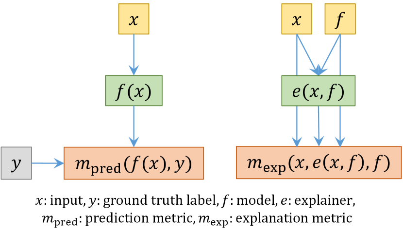
In fact, this evaluation is fundamentally different from the rest in its non-solvability, specifically due to its use of privileged information. To understand this point, let us first compare the evaluation of model prediction to that of model explanation, as illustrated in Fig. 6. The former runs the model on the input, receives the prediction, and compares it with the ground truth label, which is emphatically not available to the model under evaluation. By contrast, no such privileged information exists when computing interpretability metrics, allowing the explainer to directly solve them. In this ground truth recovery evaluation, we employ similar privileged information (i.e., induced ground truth model working mechanism) by dataset modification and model retraining. However, as discussed by Zhou et al. (2022a), such evaluations are limited to the range of ground truths that could be induced.
6 Discussion
Definition-Evaluation Duality
Our investigation demonstrates that some evaluation metrics can be used to find high-quality explanations, defined as the optimizers of the metrics. Conversely, we could also use any explanation definition as an evaluation metric . A very simple one would be , where is the explanation under evaluation, is the “reference explanation” and is a suitably chosen distance metric. It is obvious that itself achieves the optimal evaluation metric value.
Therefore, in theory, there should not be a difference of using a concept as definition vs. evaluation, but in practice, we almost always see some used mainly as definitions and others as evaluations (Fig. 2). A major reason of not considering to use evaluations as definitions could be the presumed intractability of the optimization, which is experimentally refuted in this paper, as the beam search demonstrates its efficacy and efficiency.
Conversely, why do we not see more definitions (e.g., gradients and LIME) used as evaluations? Such an attempt may sound trivial yet unjustifiable at the same time: trivial because it is equivalent to claiming that the corresponding explainer definition is the best, which is in turn a seemingly unjustifiable circular logic.
More importantly, we motivate a new research direction opened up by the duality concept. Traditionally, definitions and evaluations have been considered and developed separately, but duality suggests that any interpretability concept can be used as both. Thus, we propose that we should focus on studying the intrinsic properties of these concepts, independent of their usage as one or another. For example, are some concepts inherently superior for model explanations than others? How can we measure the similarity between two concepts? What does the space of these concepts look like? None of them are currently answerable due to a complete lack of formalization, but research on it could lead to a much deeper understanding of local explanations.
Demonstrable Utility
Given the duality, how should we evaluate explanations? Fundamentally, local explanations are used for model understanding (Zheng et al., 2022; Zhou et al., 2022b), and we advocate for evaluating demonstrable utility: the presence of an explanation compared to its absence, or the newly proposed explanation compared to existing ones, should lead to a measurable difference in some practically beneficial aspect.
For example, people use explanations to identify spurious correlation during development, audit fairness before deployment, and assist human decision makers during deployment. However, recent findings cast doubt on the feasibility of model explanations to support any of these use cases (Bansal et al., 2021; Jia et al., 2022; Zhou et al., 2022a).
Demonstrating such utilities would bypass discussions of solvability and directly assert their usefulness (Chen et al., 2022). The examples listed here are by no means comprehensive, and a systematic taxonomy is valuable. Furthermore, it is likely that no single explainer is a one-size-fit-all solution. More refined knowledge of the strengths and weaknesses of each method in supporting different aspects of model understanding is highly desirable.
7 Conclusion
We study the relationship between definitions and evaluations of local explanations. We identify the solvability property of evaluation metrics, such that for each evaluation metric, there is an explicit search procedure to find the explanation that achieves the optimal metric value. In other words, every evaluation admits a definition that solves it.
Compared to the current practice of defining a explainer and then evaluating it on a metric, solvability allows us to directly find the explanation that optimizes the target metric and guarantee a very favorable evaluation outcome. In this paper, we investigate the feasibility of this process. First, we propose to use beam search to find the explanation E∗ that optimizes for comprehensiveness and sufficiency (DeYoung et al., 2020). Then, in a suite of evaluations, we find E∗ performing comparably or favorably to existing explainers such as LIME.
Therefore, for practitioners, we recommend using the proposed explainer for computing local model explanations and provide the Python solvex package for easy adoption (App. A). For researchers, we propose a definition-evaluation duality inspired by solvability, which opens up many new research directions.
Limitations and Ethical Impact
The focus of our paper is to investigate the search-based explanation that explicitly optimizes a target quality metric. While the results suggest that it is comparable or favorable to existing heuristic explainers on various technical aspects, its societal properties have not been studied. For example, Ghorbani et al. (2019) showed that many heuristic explanations can be easily manipulated and Slack et al. (2020) demonstrated that discriminative models can be carefully modified such that their discrimination is hidden by heuristic explanations. It is possible that same issues exist for the search-based explanation, and thus we advise to carefully study them before deployment.
Another limitation of this approach is that E∗ explainer only produces rankings of feature importance, rather than numerical values of feature importance. In other words, E∗ does not distinguish whether one feature is only slightly or significantly more important than another. By comparison, almost all heuristic explainers output numerical values (e.g., magnitude of gradient). Other than the ease of search in the ranking space than the numerical value space, we give three additional reasons. First, the utility of actual values, beyond the induced rankings, has not been well studied in the literature. In addition, many popular explanation toolkits (e.g., Wallace et al., 2019) even defaults to top- visualization. Last, popular evaluation metrics rarely consider values either, suggesting that there currently lack guiding principles and desiderata for these values. Moreover, if and when such value-aware metrics are widely adopted, we could augment our optimizer with them or incorporate them into a post-processing fix without affecting the ranking, similar to the shift operation done on Line 9 of Alg. 1.
References
- Adebayo et al. (2018) Julius Adebayo, Justin Gilmer, Michael Muelly, Ian Goodfellow, Moritz Hardt, and Been Kim. 2018. Sanity checks for saliency maps. In Advances in Neural Information Processing Systems (NeurIPS), pages 9505–9515.
- Alvarez-Melis and Jaakkola (2018a) David Alvarez-Melis and Tommi S Jaakkola. 2018a. On the robustness of interpretability methods. In ICML Workshop on Human Interpretability in Machine Learning.
- Alvarez-Melis and Jaakkola (2018b) David Alvarez-Melis and Tommi S Jaakkola. 2018b. Towards robust interpretability with self-explaining neural networks. In Advances in Neural Information Processing Systems (NeurIPS), volume 31.
- Arya et al. (2019) Vijay Arya, Rachel KE Bellamy, Pin-Yu Chen, Amit Dhurandhar, Michael Hind, Samuel C Hoffman, Stephanie Houde, Q Vera Liao, Ronny Luss, Aleksandra Mojsilović, et al. 2019. One explanation does not fit all: A toolkit and taxonomy of AI explainability techniques. arXiv:1909.03012.
- Asghar (2016) Nabiha Asghar. 2016. Yelp dataset challenge: Review rating prediction. arXiv:1605.05362.
- Bansal et al. (2021) Gagan Bansal, Tongshuang Wu, Joyce Zhou, Raymond Fok, Besmira Nushi, Ece Kamar, Marco Tulio Ribeiro, and Daniel Weld. 2021. Does the whole exceed its parts? the effect of AI explanations on complementary team performance. In ACM CHI Conference on Human Factors in Computing Systems (CHI), pages 1–16.
- Bastings et al. (2022) Jasmijn Bastings, Sebastian Ebert, Polina Zablotskaia, Anders Sandholm, and Katja Filippova. 2022. A protocol for evaluating the faithfulness of input salience methods for text classification. In Conference on Empirical Methods in Natural Language Processing (EMNLP). Association for Computational Linguistics.
- Chan et al. (2022) Chun Sik Chan, Huanqi Kong, and Liang Guanqing. 2022. A comparative study of faithfulness metrics for model interpretability methods. In Annual Meeting of the Association for Computational Linguistics (ACL), pages 5029–5038. Association for Computational Linguistics.
- Chen et al. (2022) Valerie Chen, Jeffrey Li, Joon Sik Kim, Gregory Plumb, and Ameet Talwalkar. 2022. Interpretable machine learning: Moving from mythos to diagnostics. Queue, 19(6):28–56.
- Chrysostomou and Aletras (2021) George Chrysostomou and Nikolaos Aletras. 2021. Improving the faithfulness of attention-based explanations with task-specific information for text classification. In Annual Meeting of the Association for Computational Linguistics and International Joint Conference on Natural Language Processing (ACL-IJCNLP), pages 477–488. Association for Computational Linguistics.
- Dabkowski and Gal (2017) Piotr Dabkowski and Yarin Gal. 2017. Real time image saliency for black box classifiers. In Advances in Neural Information Processing Systems (NIPS), volume 30.
- Deng et al. (2009) Jia Deng, Wei Dong, Richard Socher, Li-Jia Li, Kai Li, and Li Fei-Fei. 2009. ImageNet: A large-scale hierarchical image database. In IEEE Conference on Computer Vision and Pattern Recognition (CVPR), pages 248–255. IEEE.
- DeYoung et al. (2020) Jay DeYoung, Sarthak Jain, Nazneen Fatema Rajani, Eric Lehman, Caiming Xiong, Richard Socher, and Byron C. Wallace. 2020. ERASER: A benchmark to evaluate rationalized NLP models. In Annual Meeting of the Association for Computational Linguistics (ACL), pages 4443–4458. Association for Computational Linguistics.
- Feng et al. (2018) Shi Feng, Eric Wallace, Alvin Grissom II, Mohit Iyyer, Pedro Rodriguez, and Jordan Boyd-Graber. 2018. Pathologies of neural models make interpretations difficult. In Conference on Empirical Methods in Natural Language Processing (EMNLP), pages 3719–3728. Association for Computational Linguistics.
- Geirhos et al. (2020) Robert Geirhos, Jörn-Henrik Jacobsen, Claudio Michaelis, Richard Zemel, Wieland Brendel, Matthias Bethge, and Felix A Wichmann. 2020. Shortcut learning in deep neural networks. Nature Machine Intelligence, 2(11):665–673.
- Ghorbani et al. (2019) Amirata Ghorbani, Abubakar Abid, and James Zou. 2019. Interpretation of neural networks is fragile. In AAAI Conference on Artificial Intelligence (AAAI), volume 33, pages 3681–3688.
- He et al. (2016) Kaiming He, Xiangyu Zhang, Shaoqing Ren, and Jian Sun. 2016. Deep residual learning for image recognition. In IEEE Conference on Computer Vision and Pattern Recognition (CVPR), pages 770–778. IEEE.
- Jia et al. (2022) Yan Jia, John McDermid, Tom Lawton, and Ibrahim Habli. 2022. The role of explainability in assuring safety of machine learning in healthcare. IEEE Transactions on Emerging Topics in Computing (T-ETC), 10(4):1746–1760.
- Ju et al. (2022) Yiming Ju, Yuanzhe Zhang, Zhao Yang, Zhongtao Jiang, Kang Liu, and Jun Zhao. 2022. Logic traps in evaluating attribution scores. In Annual Meeting of the Association for Computational Linguistics (ACL), pages 5911–5922. Association for Computational Linguistics.
- Kim et al. (2020) Siwon Kim, Jihun Yi, Eunji Kim, and Sungroh Yoon. 2020. Interpretation of NLP models through input marginalization. In Conference on Empirical Methods in Natural Language Processing (EMNLP), pages 3154–3167. Association for Computational Linguistics.
- Kirkpatrick et al. (1983) Scott Kirkpatrick, C Daniel Gelatt Jr, and Mario P Vecchi. 1983. Optimization by simulated annealing. Science, 220(4598):671–680.
- Kohavi and Becker (1996) Ronny Kohavi and Barry Becker. 1996. UCI Adult data set. UCI Meachine Learning Repository.
- Li et al. (2016a) Jiwei Li, Xinlei Chen, Eduard Hovy, and Dan Jurafsky. 2016a. Visualizing and understanding neural models in NLP. In Conference of the North American Chapter of the Association for Computational Linguistics: Human Language Technologies (NAACL-HLT), pages 681–691. Association for Computational Linguistics.
- Li et al. (2016b) Jiwei Li, Will Monroe, and Dan Jurafsky. 2016b. Understanding neural networks through representation erasure. arXiv:1612.08220.
- Lundberg and Lee (2017) Scott M Lundberg and Su-In Lee. 2017. A unified approach to interpreting model predictions. In Advances in Neural Information Processing Systems (NIPS), pages 4765–4774.
- Luss et al. (2021) Ronny Luss, Pin-Yu Chen, Amit Dhurandhar, Prasanna Sattigeri, Yunfeng Zhang, Karthikeyan Shanmugam, and Chun-Chen Tu. 2021. Leveraging latent features for local explanations. In ACM SIGKDD International Conference on Knowledge Discovery and Data Mining (KDD), pages 1139–1149.
- Madry et al. (2018) Aleksander Madry, Aleksandar Makelov, Ludwig Schmidt, Dimitris Tsipras, and Adrian Vladu. 2018. Towards deep learning models resistant to adversarial attacks. In International Conference on Learning Representations (ICLR).
- Nie et al. (2018) Weili Nie, Yang Zhang, and Ankit Patel. 2018. A theoretical explanation for perplexing behaviors of backpropagation-based visualizations. In International Conference on Machine Learning (ICML), pages 3809–3818.
- Petsiuk et al. (2018) Vitali Petsiuk, Abir Das, and Kate Saenko. 2018. RISE: Randomized input sampling for explanation of black-box models. In British Machine Vision Conference (BMVC).
- Pham et al. (2022) Thang Pham, Trung Bui, Long Mai, and Anh Nguyen. 2022. Double trouble: How to not explain a text classifier’s decisions using counterfactuals synthesized by masked language models? In Conference of the Asia-Pacific Chapter of the Association for Computational Linguistics and International Joint Conference on Natural Language Processing (AACL-IJCNLP), pages 12–31. Association for Computational Linguistics.
- Plumb et al. (2018) Gregory Plumb, Denali Molitor, and Ameet S Talwalkar. 2018. Model agnostic supervised local explanations. In Advances in Neural Information Processing Systems (NeurIPS).
- Ribeiro et al. (2016) Marco Tulio Ribeiro, Sameer Singh, and Carlos Guestrin. 2016. "Why should I trust you?" explaining the predictions of any classifier. In ACM SIGKDD International Conference on Knowledge Discovery and Data Mining (KDD), pages 1135–1144.
- Roth (1988) Alvin E Roth. 1988. The Shapley Value: Essays in Honor of Lloyd S. Shapley. Cambridge University Press.
- Samek et al. (2016) Wojciech Samek, Alexander Binder, Grégoire Montavon, Sebastian Lapuschkin, and Klaus-Robert Müller. 2016. Evaluating the visualization of what a deep neural network has learned. IEEE Transactions on Neural Networks and Learning Systems (T-NNLS), 28(11):2660–2673.
- Serrano and Smith (2019) Sofia Serrano and Noah A. Smith. 2019. Is attention interpretable? In Annual Meeting of the Association for Computational Linguistics (ACL), pages 2931–2951. Association for Computational Linguistics.
- Simonyan et al. (2013) Karen Simonyan, Andrea Vedaldi, and Andrew Zisserman. 2013. Deep inside convolutional networks: Visualising image classification models and saliency maps. arXiv:1312.6034.
- Slack et al. (2020) Dylan Slack, Sophie Hilgard, Emily Jia, Sameer Singh, and Himabindu Lakkaraju. 2020. Fooling LIME and SHAP: Adversarial attacks on post hoc explanation methods. In AAAI/ACM Conference on AI, Ethics, and Society (AIES), pages 180–186. Association for Computing Machinery.
- Smilkov et al. (2017) Daniel Smilkov, Nikhil Thorat, Been Kim, Fernanda Viégas, and Martin Wattenberg. 2017. SmoothGrad: Removing noise by adding noise. arXiv:1706.03825.
- Socher et al. (2013) Richard Socher, Alex Perelygin, Jean Wu, Jason Chuang, Christopher D Manning, Andrew Y Ng, and Christopher Potts. 2013. Recursive deep models for semantic compositionality over a sentiment treebank. In Conference on Empirical Methods in Natural Language Processing (EMNLP), pages 1631–1642. Association for Computational Linguistics.
- Sundararajan et al. (2017) Mukund Sundararajan, Ankur Taly, and Qiqi Yan. 2017. Axiomatic attribution for deep networks. In International Conference on Machine Learning (ICML), pages 3319–3328.
- Wallace et al. (2019) Eric Wallace, Jens Tuyls, Junlin Wang, Sanjay Subramanian, Matt Gardner, and Sameer Singh. 2019. AllenNLP Interpret: A framework for explaining predictions of NLP models. In Conference on Empirical Methods in Natural Language Processing and International Joint Conference on Natural Language Processing (EMNLP-IJCNLP): System Demonstrations, pages 7–12. Association for Computational Linguistics.
- Winkler et al. (2019) Julia K Winkler, Christine Fink, Ferdinand Toberer, Alexander Enk, Teresa Deinlein, Rainer Hofmann-Wellenhof, Luc Thomas, Aimilios Lallas, Andreas Blum, Wilhelm Stolz, et al. 2019. Association between surgical skin markings in dermoscopic images and diagnostic performance of a deep learning convolutional neural network for melanoma recognition. JAMA Dermatology, 155(10):1135–1141.
- Zeiler and Fergus (2014) Matthew D Zeiler and Rob Fergus. 2014. Visualizing and understanding convolutional networks. In European Conference on Computer Vision (ECCV), pages 818–833. Springer.
- Zhang et al. (2019) Hao Zhang, Jiayi Chen, Haotian Xue, and Quanshi Zhang. 2019. Towards a unified evaluation of explanation methods without ground truth. arXiv preprint arXiv:1911.09017.
- Zheng et al. (2022) Yiming Zheng, Serena Booth, Julie Shah, and Yilun Zhou. 2022. The irrationality of neural rationale models. In 2nd Workshop on Trustworthy Natural Language Processing (TrustNLP). Association for Computational Linguistics.
- Zhou et al. (2022a) Yilun Zhou, Serena Booth, Marco Tulio Ribeiro, and Julie Shah. 2022a. Do feature attribution methods correctly attribute features? In AAAI Conference on Artificial Intelligence (AAAI).
- Zhou et al. (2021) Yilun Zhou, Adithya Renduchintala, Xian Li, Sida Wang, Yashar Mehdad, and Asish Ghoshal. 2021. Towards understanding the behaviors of optimal deep active learning algorithms. In International Conference on Artificial Intelligence and Statistics (AISTATS), pages 1486–1494.
- Zhou et al. (2022b) Yilun Zhou, Marco Tulio Ribeiro, and Julie Shah. 2022b. ExSum: From local explanations to model understanding. In Conference of the North American Chapter of the Association for Computational Linguistics: Human Language Technologies (NAACL-HLT). Association for Computational Linguistics.
Appendix A The Python solvex Package
We release the Python solvex package implementing explainer in a model-agnostic manner. The project website at https://yilunzhou.github.io/solvability/ contains detailed tutorials and documentation. Here, we showcase three additional use cases of the explainer.
To explain long paragraphs, feature granularity at the level of sentences may be sufficient or even desired. solvex can use spaCy333https://spacy.io/ to split a paragraph into sentences and compute the sentence-level attribution explanation accordingly. As an explanation, Fig. 7 shows an explanation for the prediction on a test instance in the Yelp dataset (Asghar, 2016) made by the albert-base-v2-yelp-polarity model.
Contrary to other reviews, I have zero complaints about the service or the prices. I have been getting tire service here for the past 5 years now, and compared to my experience with places like Pep Boys, these guys are experienced and know what they’re doing. Also, this is one place that I do not feel like I am being taken advantage of, just because of my gender. Other auto mechanics have been notorious for capitalizing on my ignorance of cars, and have sucked my bank account dry. But here, my service and road coverage has all been well explained - and let up to me to decide. And they just renovated the waiting room. It looks a lot better than it did in previous years.
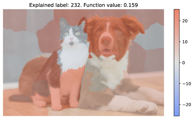
This package can explain image predictions with superpixel features (similar to LIME (Ribeiro et al., 2016)). Fig. 8 shows the explanation for the top prediction (Class 232: Border Collie, a dog breed) by the ResNet-50 (He et al., 2016) trained on ImageNet (Deng et al., 2009).
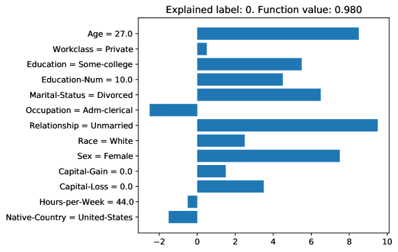
Last, it can also explain models trained on tabular datasets with both categorical and numerical features. For a random forest model trained on the Adult dataset (Kohavi and Becker, 1996), Fig. 9 shows the attribution on each feature that contributes to the class 0 (i.e., income less than or equal to ). Note that a more positive attribution value indicates that the feature (e.g. age or relationship) contributes more to the low income prediction.
Appendix B The Definition-Evaluation Spectrum and Its Various Concepts
We describe the reasoning of assigning each concept to its location on the definition-evaluation spectrum (Fig. 2, reproduced as Fig. 10 below), as currently perceived by the community according to our understanding. Note that the discussion is unavoidably qualitative, but we hope that it illustrates the general idea of this spectrum.

We start on the definition side, where the gradient saliency (Simonyan et al., 2013; Li et al., 2016a) is a classic feature attribution definition but, to the best of our knowledge, has never been used in any evaluation capacity. Moving towards the evaluation side, we have LIME (Ribeiro et al., 2016), which is again used mainly to define explanations (as linear regression coefficients), but the notion of local fidelity introduced by LIME has been occasionally used to evaluate other explainers as well (Plumb et al., 2018). Similar to LIME, SHAP (Lundberg and Lee, 2017) defines explanations as those that (approximately) satisfy the Shapley axioms (Roth, 1988), which can also be used to evaluate how well a certain explanation performs with respect to these axioms (Zhang et al., 2019). Next up we have the occlusion concept, which, as seen in Sec. 2, can be used as one explainer definition, Occl (Zeiler and Fergus, 2014; Li et al., 2016b), and two (not so popular) evaluations, DFMIT (Chrysostomou and Aletras, 2021) and RankDel (Alvarez-Melis and Jaakkola, 2018b).
Further on the evaluation side, we now encounter concepts that are more often used for evaluations than definitions. Robustness (Ghorbani et al., 2019) evaluates the similarity between explanations among similar inputs and a higher degree of similarity is often more desirable (Alvarez-Melis and Jaakkola, 2018a). However, this robustness desideratum is incorporated explicitly into some explainers, such as via the noise aggregation in SmoothGrad (Smilkov et al., 2017). On the right-most end we have sufficiency and comprehensiveness (DeYoung et al., 2020), which evaluates whether keeping a small subset of features could lead to the original model prediction, or removing it could lead to a large drop in model prediction. They are arguably the most popular among various evaluation metrics, and have been repeatedly proposed under different names such as the area over perturbation curve (AoPC) (Samek et al., 2016) and insertion/deletion metrics (Petsiuk et al., 2018). Using such these two ideas for definitions are relatively rare, with one notable exception of smallest sufficient/destroying regions (SSR/SDR) proposed by (Dabkowski and Gal, 2017).
Overall, it is clear that the community considers certain concepts more for definitions and others more for evaluations, which motivates the investigation for this paper and future work: can we swap the definition/evaluation roles, and if so, what are the implications?
Appendix C Additional Qualitative Examples of the E∗ Explanation
Fig. 11 presents more visualizations of E∗ explanations. These examples suggest that E∗ mostly focus on words that convey strong sentiments, which is a plausible working mechanism of a sentiment classifier.
A triumph , relentless and beautiful in its downbeat darkness .
Ranks among Willams ’ best screen work .
Zany , exuberantly irreverent animated space adventure .
Behind the snow games and lovable Siberian huskies ( plus one sheep dog ) , the picture hosts a parka-wrapped dose of heart .
… a haunting vision , with images that seem more like disturbing hallucinations .
Suffocated at conception by its Munchausen-by-proxy mum .
It ’s an awfully derivative story .
A dreadful live-action movie .
Appendix D An Analysis on the RankIns Metric
As introduced in App. 2, RankDel evaluates the monotonicity of the model prediction curve when more important features are successively inserted into an empty input. While this expectation seems reasonable, it suffers from a critical issue due to the convention in ranking features: if a feature contributes against the prediction, such as a word of sentiment opposite to the prediction (e.g., a positive prediction on “Other than the story plot being a bit boring, everything else is actually masterfully designed and executed.”), it should have negative attribution and the convention is to put them lower in the rank (i.e., less important) than those have zero contributions. This implementation leads to the correct interpretation of all other metric values.
However, under this convention, the first few words added to the empty input should decrease the model prediction and then increase it, leading to a U-shaped curve. In fact, it is the comprehensiveness curve shown in Fig. 4, flipped both horizontally (because features are inserted rather than removed) and vertically (because the plotted quantity is the model prediction rather than change in prediction). Thus, a deeper U-shape should be preferred, but it is less monotonic. This also explains why the random attribution baseline achieves such a high ranking correlation: as we randomly add features from the empty string to the full input, on average the curve should be a more or less monotonic interpolation between model predictions on empty and full inputs, which has better monotonicity rank correlation than the U-shape.
It is not clear how to fix the metric. Previous works that proposed (Luss et al., 2021) or used (Chan et al., 2022) this metric often ignored the issue. One work (Arya et al., 2019) filtered out all features of negative attribution values and evaluate the rank correlation only on the rest. This, however, is easily manipulatable by an adversary. Specifically, an explainer could shift all attribution values down such that only the most positive one has a non-negative value. This change results in a perfect correlation as long as removing most positive feature induces a decrease in model prediction – an especially low requirement to satisfy. Empirically, we found that inserting features based on their (unsigned) magnitude barely affects the result either. Thus, we argue that this metric is not a good measurement of explanation quality.
Appendix E Visualization of Perturbation Effects
Fig. 12 visually presents the random perturbation, with different standard deviation of the Gaussian noise. In each panel, the top row orders the features by their ranked importance, from least important on the left to most on the right, and the bottom row orders the features with perturbed ranked importance, with lines connecting to their original position. For example, in the top panel for , the perturbation swaps the relative order of the two least important features on the left.
Appendix F Another Assessment on the Explainer-Attacking-Model Behavior
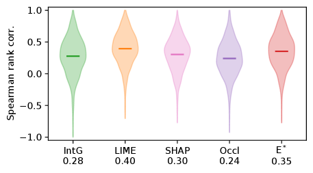
We describe another experiment to assess whether the explanations exploit the adversarial vulnerability of the model. While it is possible that the model could use some shortcuts (Geirhos et al., 2020), we would expect it to predominantly use sentiment-conveying words, as it achieves high accuracy and no such shortcuts are known for the dataset. In this case, we should expect an explainer that does not adversarially exploit the model to give attributions for words correlated with their sentiment values, while an explainer that attacks the model would rate words that are “adversarial bugs” to be more important.
Conveniently, the SST dataset provides human annotations of the polarity score between 0 and 1 for each word, where 0 means very negative, 1 means very positive, and 0.5 means neutral. We compute the alignment between the attribution values (for the positive class) and this score for each word. Given a sentence with explanation and word polarity score , the alignment is defined as the Spearman rank correlation coefficient . Since the vanilla gradient only produces non-negative values, it is impossible to identify whether a word contributes to or against the positive class, and we exclude it from the analysis.
Fig. 13 plots the distribution of rank correlations among the test set instances, with the average shown as the bar and also annotated on the horizontal axis. Although no method achieves very high alignment, E∗ is the second-highest, after LIME. Thus, giving out assumption that high-polarity words are the indeed genuine signals used by the model for making predictions, we can conclude that E∗ does not adversarially exploit the model for its vulnerability any more severely than the heuristic explainers.