The strong convergence phenomenon

Ramon van Handel Department of Mathematics, Princeton University, Princeton, NJ 08544, USA rvan@math.princeton.edu

Abstract.

In a seminal 2005 paper, Haagerup and Thorbjørnsen discovered that the norm of any noncommutative polynomial of independent complex Gaussian random matrices converges to that of a limiting family of operators that arises from Voiculescu’s free probability theory. In recent years, new methods have made it possible to establish such strong convergence properties in much more general situations, and to obtain even more powerful quantitative forms of the strong convergence phenomenon. These, in turn, have led to a number of spectacular applications to long-standing open problems on random graphs, hyperbolic surfaces, and operator algebras, and have provided flexible new tools that enable the study of random matrices in unexpected generality. This survey aims to provide an introduction to this circle of ideas.

2010 Mathematics Subject Classification:

60B20; 15B52; 46L53; 46L54

1. Introduction

The aim of this survey is to discuss recent developments surrounding the following phenomenon, which has played a central role in a series of breakthroughs in the study of random graphs, hyperbolic surfaces, and operator algebras.

Definition 1.1.

Let $\bm{X}^{N}=(X_{1}^{N},\ldots,X_{r}^{N})$ be a sequence of $r$ -tuples of random matrices of increasing dimension, and let $\bm{x}=(x_{1},\ldots,x_{r})$ be an $r$ -tuple of bounded operators on a Hilbert space. Then $\bm{X}^{N}$ is said to converge strongly to $\bm{x}$ if

\lim_{N\to\infty}\|P(\bm{X}^{N},\bm{X}^{N*})\|=\|P(\bm{x},\bm{x}^{*})\|\quad\text{in probability}

for every $D\in\mathbb{N}$ and $P\in\mathrm{M}_{D}(\mathbb{C})\otimes\mathbb{C}\langle x_{1},\ldots,x_{2r}\rangle$ .

Here we recall that a noncommutative polynomial with matrix coefficients $P\in\mathrm{M}_{D}(\mathbb{C})\otimes\mathbb{C}\langle x_{1},\ldots,x_{r}\rangle$ of degree $q$ is a formal expression

P(x_{1},\ldots,x_{r})=A_{0}\otimes\mathbf{1}+\sum_{k=1}^{q}\sum_{i_{1},\ldots,i_{k}=1}^{r}A_{i_{1},\ldots,i_{k}}\otimes x_{i_{1}}\cdots x_{i_{k}},

where $A_{i_{1},\ldots,i_{k}}\in\mathrm{M}_{D}(\mathbb{C})$ are $D\times D$ complex matrices. Such a polynomial defines a bounded operator whenever bounded operators are substituted for the free variables $x_{1},\ldots,x_{r}$ . When $D=1$ , this reduces to the classical notion of a noncommutative polynomial (we will then write $P\in\mathbb{C}\langle x_{1},\ldots,x_{r}\rangle$ ).

The significance of the strong convergence phenomenon may not be immediately obvious when it is encountered for the first time. Let us therefore begin with a very brief discussion of its origins.

The modern study of the spectral theory of random matrices arose from the work of physicists, especially that of Wigner and Dyson in the 1950s and 60s [129]. Random matrices arise here as generic models for real physical systems that are too complicated to be understood in detail, such as the energy level structure of complex nuclei. It is believed that universal features of such systems are captured by random matrix models that are chosen essentially uniformly within the appropriate symmetry class. Such questions have led to numerous developments in probability and mathematical physics, and the spectra of such models are now understood in stunning detail down to microscopic scales (see, e.g., [46]).

In contrast to these physically motivated models, random matrices that arise in other areas of mathematics often possess a much less regular structure. One way to build complex models is to consider arbitrary noncommutative polynomials of independent random matrices drawn from simple random matrix ensembles. It was shown in the seminal work of Voiculescu [126] that the limiting empirical eigenvalue distribution of such matrices can be described in terms of a family of limiting operators obtained by a free product construction. This is a fundamentally new perspective: while traditional random matrix methods are largely based on asymptotic explicit expressions or self-consistent equations satisfied by certain spectral statistics, Voiculescu’s theory provides us with genuine limiting objects whose spectral statistics are, in many cases, amenable to explicit computations. The interplay between random matrices and their limiting objects has proved to be of central importance, and will play a recurring role in the sequel.

While Voiculescu’s theory is extremely useful, it yields rather weak information in that it can only describe the asympotics of the trace of polynomials of random matrices. It was a major breakthrough when Haagerup and Thorbjørnsen [60] showed, for complex Gaussian (GUE) random matrices, that also the norm of arbitrary polynomials converges to that of the corresponding limiting object. This much more powerful property, which was the first instance of strong convergence, opened the door to many subsequent developments.

The works of Voiculescu and Haagerup–Thorbjørnsen were directly motivated by applications to the theory of operator algebras. The fact that polynomials of a family of operators can be approximated by matrices places strong constraints on the operator (von Neumann- or $C^{*}$ -)algebras generated by this family: roughly speaking, it ensures that such algebras are “approximately finite-dimensional” in a certain sense. These properties have led to the resolution of important open problems in the theory of operator algebras which do not a priori have anything to do with random matrices; see, e.g., [128, 99, 60].

The interplay between operator algebras and random matrices continues to be a rich source of problems in both areas; an influential recent example is the work of Hayes [65] on the Peterson–Thom conjecture (cf. section 5.4). In recent years, however, the notion of strong convergence has led to spectacular new applications in several other areas of mathematics. Broadly speaking, the importance of the strong convergence phenomenon is twofold.

$\bullet$

Noncommutative polynomials are highly expressive: many complex structures can be encoded in terms of spectral properties of noncommutative polynomials.
$\bullet$

Norm convergence is an extremely strong property, which provides access to challenging features of complex models.

Furthermore, new mathematical methods have made it possible to establish novel quantitative forms of strong convergence, which enable the treatment of even more general random matrix models that were previously out of reach.

We will presently highlight a number of themes that illustrate recent applications and developments surrounding strong convergence. The remainder of this survey is devoted to a more detailed introduction to this circle of ideas.

It should be emphasized at the outset that while I have aimed to give a general introduction to the strong convergence phenomenon and related topics, this survey is selectively focused on recent developments that are closest to my own interests, and is by no means comprehensive or complete. The interested reader may find complementary perspectives in surveys of Magee [88] and Collins [39], and is warmly encouraged to further explore the research literature on this subject.

1.1. Optimal spectral gaps

Let $G^{N}$ be a $d$ -regular graph with $N$ vertices. By the Perron-Frobenius theorem, its adjacency matrix $A^{N}$ has largest eigenvalue $\lambda_{1}(A)=d$ with eigenvector $1$ (the vector all of whose entries are one). The remaining eigenvalues are bounded by

\|A^{N}|_{1^{\perp}}\|=\max_{i=2,\ldots,N}|\lambda_{i}(A^{N})|\leq d.

The smaller this quantity, the faster does a random walk on $G^{N}$ mix. The following classical lemma yields a lower bound that holds for any sequence of $d$ -regular graphs. It provides a speed limit on how fast random walks can mix.

Lemma 1.2 (Alon–Boppana).

For any $d$ -regular graphs $G^{N}$ with $N$ vertices,

\|A^{N}|_{1^{\perp}}\|\geq 2\sqrt{d-1}-o(1)\quad\text{as}\quad N\to\infty.

Given a universal lower bound on the nontrivial eigenvalues, the obvious question is whether there exist graphs that attain this bound. Such graphs have the largest possible spectral gap. One may expect that such heavenly graphs must be very special, and indeed the first examples of such graphs were carefully constructed using deep number-theoretic ideas by Lubotzky–Phillips–Sarnak [87] and Margulis [97]. It may therefore seem surprising that this property does not turn out to be all that special at all: random graphs have an optimal spectral gap [50].¹¹1Here we gloss over an important distinction between the explicit and random constructions: the former yields the so-called Ramanujan property $\|A^{N}|_{1^{\perp}}\|\leq 2\sqrt{d-1}$ , while the latter yields only $\|A^{N}|_{1^{\perp}}\|\leq 2\sqrt{d-1}+o(1)$ which is the natural converse to Lemma 1.2 (cf. section 6.5).

Theorem 1.3 (Friedman).

For a random $d$ -regular graph $G^{N}$ on $N$ vertices,

\|A^{N}|_{1^{\perp}}\|\leq 2\sqrt{d-1}+o(1)\quad\text{with probability}\quad 1-o(1)\quad\text{as}\quad N\to\infty.

We now explain that Theorem 1.3 may be viewed as a very special instance of strong convergence. This viewpoint will open the door to establishing optimal spectral gaps in much more general situations.

Let us begin by recalling that the proof of Lemma 1.2 is based on the simple observation that for any graph $G$ , the number of closed walks with a given length and starting vertex is lower bounded by the number of such walks in its universal cover $\tilde{G}$ . When $G$ is $d$ -regular, its universal cover $\tilde{G}$ is the infinite $d$ -regular tree. From this, it is not difficult to deduce that the maximum nontrivial eigenvalue of a $d$ -regular graph is asymptotically lower bounded by the spectral radius of the infinite $d$ -regular tree, which is $2\sqrt{d-1}$ [71, §5.2.2].

Theorem 1.3 therefore states, in essence, that the support of the nontrivial spectrum of a random $d$ -regular graph behaves as that of the infinite $d$ -regular tree. To make the connection more explicit, it is instructive to construct both the random graph and infinite tree in a parallel manner. For simplicity, we assume $d$ is even (the construction can be modified to the odd case as well).

Figure 1.1. Left figure:

4

-regular graph generated by two permutations. Right figure:

4

-regular tree generated by two free generators

a,b

of the free group

\mathbf{F}_{2}

. The edges defined by the two generators are colored red and blue, respectively.

Given a permutation $\sigma\in\mathbf{S}_{N}$ , we can define edges between $N$ vertices by connecting each vertex $k\in[N]$ to its neighbors $\sigma(k)$ and $\sigma^{-1}(k)$ . This defines a $2$ -regular graph. To define a $d$ -regular graph, we repeat this process with $r=\frac{d}{2}$ permutations. If the permutations are chosen independently and uniformly at random from $\mathbf{S}_{N}$ , we obtain a random $d$ -regular graph with adjacency matrix

A^{N}=U_{1}^{N}+U_{1}^{N*}+\cdots+U_{r}^{N}+U_{r}^{N*},

where $U_{i}^{N}$ are i.i.d. random permutation matrices of dimension $N$ .²²2This is the permutation model of random graphs; see [50, p. 3] for its relation to other models.

To construct the infinite $d$ -regular tree in a parallel manner, we identify the vertices of the tree with the free group $\mathbf{F}_{r}$ with $r=\frac{d}{2}$ free generators $g_{1},\ldots,g_{r}$ . Each vertex $w\in\mathbf{F}_{r}$ is then connected to its neighbors $g_{i}w$ and $g_{i}^{-1}w$ for $i=1,\ldots,r$ . This defines a $d$ -regular tree with adjacency matrix

a=u_{1}+u_{1}^{*}+\cdots+u_{r}+u_{r}^{*},

where $u_{i}=\lambda(g_{i})$ is defined by the left-regular representation $\lambda:\mathbf{F}_{r}\to B(l^{2}(\mathbf{F}_{r}))$ , i.e., $\lambda(g)\delta_{w}=\delta_{gw}$ where $\delta_{w}\in l^{2}(\mathbf{F}_{r})$ is the coordinate vector of $w\in\mathbf{F}_{r}$ .

These models are illustrated in Figure 1.1 for $r=2$ , where the edges are colored according to their generator; e.g., $U_{1}+U_{1}^{*}$ and $u_{1}+u_{1}^{*}$ are the adjacency matrices of the red edges in the left and right figures, respectively.

In these terms, Theorem 1.3 states that

\lim_{N\to\infty}\|(U_{1}^{N}+U_{1}^{N*}+\cdots+U_{r}^{N}+U_{r}^{N*})|_{1^{\perp}}\|=\|u_{1}+u_{1}^{*}+\cdots+u_{r}+u_{r}^{*}\|

in probability. This is precisely the kind of convergence described by Definition 1.1, but only for one very special polynomial

P(\bm{x},\bm{x}^{*})=x_{1}+x_{1}^{*}+\cdots+x_{r}+x_{r}^{*}.

Making a leap of faith, we can now ask whether the same conclusion might even hold for every noncommutative polynomial $P$ . That this is indeed the case is a remarkable result of Bordenave and Collins [19].

Theorem 1.4 (Bordenave–Collins).

Let $\bm{U}^{N}=(U_{1}^{N},\ldots,U_{r}^{N})$ and $\bm{u}=(u_{1},\ldots,u_{r})$ be defined as above. Then $\bm{U}^{N}|_{1^{\perp}}$ converges strongly to $\bm{u}$ , that is,

\lim_{N\to\infty}\|P(\bm{U}^{N},\bm{U}^{N*})|_{1^{\perp}}\|=\|P(\bm{u},\bm{u}^{*})\|\quad\text{in probability}

for every $D\in\mathbb{N}$ and $P\in\mathrm{M}_{D}(\mathbb{C})\otimes\mathbb{C}\langle x_{1},\ldots,x_{2r}\rangle$ .³³3The reason that we must restrict to $1^{\perp}$ is elementary: the matrices $U_{i}^{N}$ have a Perron-Frobenius eigenvector $1$ , but the operators $u_{i}$ do not as $1\not\in l^{2}(\mathbf{F}_{r})$ (an infinite vector of ones is not in $l^{2}$ ). Thus we must remove the Perron-Frobenius eigenvector to achieve strong convergence.

Theorem 1.4 is a powerful tool because many problems can be encoded as special cases of this theorem by a suitable choice of $P$ . To illustrate this, let us revisit the optimal spectral gap phenomenon in a broader context.

In general terms, the optimal spectral gap phenomenon is the following. The spectrum of various kinds of geometric objects admits a universal bound in terms of that of their universal covering space. The question is then whether there exist such objects which meet this bound. In particular, we may ask whether that is the case for random constructions. Lemma 1.2 and Theorem 1.3 establish this for regular graphs. An analogous picture in other situations is much more recent:

$\bullet$

It was shown by Greenberg [71, Theorem 6.6] that for any sequence of finite graphs $G^{N}$ with diverging number of vertices that have the same universal cover $\tilde{G}$ , the maximal nontrivial eigenvalue of $G^{N}$ is asymptotically lower bounded by the spectral radius of $\tilde{G}$ . On the other hand, given any (not necessarily regular) finite graph $G$ , there is a natural construction of random lifts $G^{N}$ with the same universal cover $\tilde{G}$ [71, §6.1]. It was shown by Bordenave and Collins [19] that an optimal spectral gap phenomenon holds for random lifts of any graph $G$ .
$\bullet$

Any hyperbolic surface $X$ has the hyperbolic plane $\mathbb{H}$ as its universal cover. Huber [77] and Cheng [35] showed that for any sequence $X^{N}$ of closed hyperbolic surfaces with diverging diameter, the first nontrivial eigenvalue of the Laplacian $\Delta_{X^{N}}$ is upper bounded by the bottom of the spectrum of $\Delta_{\mathbb{H}}$ . Whether this bound can be attained was an old question of Buser [29]. An affirmative answer was obtained by Hide and Magee [69] by showing that an optimal spectral gap phenomenon holds for random covering spaces of hyperbolic surfaces.

The key ingredient in these breakthroughs is that the relevant spectral properties can be encoded as special instances of Theorem 1.4. How this is accomplished will be sketched in sections 5.1 and 5.2. In section 5.5, we will sketch another remarkable application due to Song [122] to minimal surfaces.

Another series of developments surrrounding optimal spectral gaps arises from a different perspective on Theorem 1.4. The map $\mathrm{std}_{N}:\mathbf{S}_{N}\to\mathrm{M}_{N-1}(\mathbb{C})$ that assigns to each permutation $\sigma\in\mathbf{S}_{N}$ the restriction of the associated $N\times N$ permutation matrix to $1^{\perp}$ defines an irreducible representation of the symmetric group $\mathbf{S}_{N}$ of dimension $N-1$ called the standard representation. Thus

U_{i}^{N}|_{1^{\perp}}=\mathrm{std}_{N}(\sigma_{i}^{N}),

where $\sigma_{1}^{N},\ldots,\sigma_{r}^{N}$ are independent uniformly distributed elements of $\mathbf{S}_{N}$ . One may ask whether strong convergence remains valid if $\mathrm{std}_{N}$ is replaced by other representations $\pi_{N}$ of $\mathbf{S}_{N}$ . This and related optimal spectral gap phenomena in representation-theoretic settings are the subject of long-standing questions and conjectures; see, e.g., [119] and the references therein.

Recent advances in the study of strong convergence have led to major progress in the understanding of such questions [21, 32, 33, 90, 30]. One of the most striking results in this direction to date is the recent work of Cassidy [30], who shows that strong convergence for the symmetric group holds uniformly for all nontrivial irreducible representations of $\mathbf{S}_{N}$ of dimension up to $\exp(N^{\frac{1}{12}-\delta})$ .⁴⁴4For comparison, all irreducible representations of $\mathbf{S}_{N}$ have dimension $\exp(O(N\log N))$ . This makes it possible, for example, to study natural models of random regular graphs that achieve optimal spectral gaps using far less randomness than is required by Theorem 1.4. We will discuss these results in more detail in section 5.3.

1.2. Intrinsic freeness

We now turn to an entirely different development surrounding strong convergence that has enabled a sharp understanding of a very large class of random matrices in unexpected generality.

To set the stage for this development, let us begin by recalling the original strong convergence result of Haagerup and Thorbjørnsen [60]. Let $G_{1}^{N},\ldots,G_{r}^{N}$ be independent GUE matrices, that is, $N\times N$ self-adjoint complex Gaussian random matrices whose off-diagonal elements have variance $\frac{1}{N}$ and whose distribution is invariant under unitary conjugation. The associated limiting object is a free semicircular family $s_{1},\ldots,s_{r}$ (cf. section 4.1). Define the random matrix

X^{N}=A_{0}\otimes\mathbf{1}+\sum_{i=1}^{r}A_{i}\otimes G_{i}^{N}

and the limiting operator

X_{\rm free}=A_{0}\otimes\mathbf{1}+\sum_{i=1}^{r}A_{i}\otimes s_{i},

where $A_{0},\ldots,A_{r}\in\mathrm{M}_{D}(\mathbb{C})$ are self-adjoint matrix coefficients.

Theorem 1.5 (Haagerup–Thorbjørnsen).

For $X^{N}$ and $X_{\rm free}$ defined as above,⁵⁵5Here $\mathrm{sp}(X)$ denotes the spectrum of $X$ , and we recall that the Hausdorff distance between sets $A,B\subseteq\mathbb{R}$ is defined as $\mathrm{d_{H}}(A,B)=\inf\{\varepsilon>0:A\subseteq B+[-\varepsilon,\varepsilon]\text{ and }B\subseteq A+[-\varepsilon,\varepsilon]\}$ .

\lim_{N\to\infty}\mathrm{d_{H}}\big{(}\mathrm{sp}(X^{N}),\mathrm{sp}(X_{\rm free})\big{)}=0\quad\text{a.s.}

It is a nontrivial fact, known as the linearization trick, that Theorem 1.5 implies that $\bm{G}^{N}=(G_{1}^{N},\ldots,G_{r}^{N})$ converges strongly to $\bm{s}=(s_{1},\ldots,s_{r})$ ; see section 2.5. This conclusion was used by Haagerup and Thorbjørnsen to prove an old conjecture that the $\mathrm{Ext}$ invariant of the reduced $C^{*}$ -algebra of any countable free group with at least two generators is not a group. For our present purposes, however, the above formulation of Theorem 1.5 will be the most natural.

The result of Haagerup–Thorbjørnsen may be viewed as a strong incarnation of Voiculescu’s asymptotic freeness principle [126]. The limiting operators $s_{1},\ldots,s_{r}$ arise from a free product construction and are thus algebraically free (in fact, they are freely independent in the sense of Voiculescu). This makes it possible to compute the spectral statistics of $X_{\rm free}$ by means of closed form equations, cf. section 4.1. The explanation for Theorem 1.5 provided by the asymptotic freeness principle is that since the random matrices $G_{i}^{N}$ have independent uniformly random eigenbases (due to their unitary invariance), they become increasingly noncommutative as $N\to\infty$ which leads them to behave freely in the limit.

From the perspective of applications, however, the most interesting case of this model is the special case $N=1$ , that is, the random matrix $X=X^{1}$ defined by

X=A_{0}+\sum_{i=1}^{r}A_{i}g_{i}

where $g_{i}$ are independent standard Gaussians. Indeed, any $D\times D$ self-adjoint random matrix with jointly Gaussian entries (with arbitrary mean and covariance) can be expressed in this form. This model therefore captures almost arbitrarily structured random matrices: if one could understand random matrices at this level of generality, one would capture in one fell swoop a huge class of models that arise in applications. However, since the $1\times 1$ matrices $g_{i}=G_{i}^{1}$ commute, the asymptotic freeness principle has no bearing on such matrices, and there is no reason to expect that $X_{\rm free}$ has any significance for the behavior of $X$ .

It is therefore rather surprising that the spectral properties of arbitrarily structured Gaussian random matrices $X$ are nonetheless captured by those of $X_{\rm free}$ in great generality. This phenomenon, developed in joint works of the author with Bandeira, Boedihardjo, Cipolloni, and Schröder [10, 11], is captured by the following counterpart of Theorem 1.5 (stated here in simplified form).

Theorem 1.6 (Intrinsic freeness).

For $X$ and $X_{\rm free}$ be defined as above, we have

\mathbf{P}\big{[}\mathrm{d_{H}}\big{(}\mathrm{sp}(X),\mathrm{sp}(X_{\rm free})\big{)}>C\tilde{v}(X)\big{(}(\log D)^{\frac{3}{4}}+t\big{)}\big{]}\leq e^{-t^{2}}

for all $t\geq 0$ . Here $C$ is a universal constant,

\tilde{v}(X)=\|\mathbf{E}[(X-\mathbf{E}X)^{2}]\|^{\frac{1}{4}}\|\mathrm{Cov}(X)\|^{\frac{1}{4}},

and $\mathrm{Cov}(X)$ is the $D^{2}\times D^{2}$ covariance matrix of the entries of $X$ .

Remark 1.7.

While Theorem 1.6 captures the edges of the spectrum of $X$ , analogous results for other spectral parameters (such as the spectral distribution) may be found in [10, 11]. These results are further extended to a large class of non-Gaussian random matrices in joint work of the author with Brailovskaya [23].

Theorem 1.6 states that the spectrum of $X$ behaves like that of $X_{\rm free}$ as soon at the parameter $\tilde{v}(X)$ is small. Unlike for the model $X^{N}$ , where noncommutativity is overtly introduced by means of unitarily invariant matrices, the mechanism for $X$ to behave as $X_{\rm free}$ can only arise from the structure of the matrix coefficients $A_{0},\ldots,A_{r}$ . We call this phenomenon intrinsic freeness. It should not be obvious at this point why the parameter $\tilde{v}(X)$ captures intrinsic freeness; the origin of this phenomenon (which was inspired in part by [60, 125]) and the mechanism that gives rise to it will be discussed in section 4.

In practice, Theorem 1.6 proves to be a powerful result as $\tilde{v}(X)$ is indeed small in numerous applications, while the result applies without any structural assumptions on the random matrix $X$ . This is especially useful in questions of applied mathematics, where messy random matrices are par for the course. Several such applications are illustrated, for example, in [11, §3].

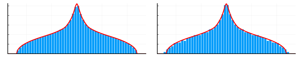
Refer to caption — Figure 1.2. Example of $P(H_{1}^{N},H_{2}^{N},H_{3}^{N})$ where $H_{i}^{N}$ are independent $N\times N$ GUE (left plot) or $w$ -sparse band matrices (right plot) with $N=1000$ and $w=27$ . The histograms show the eigenvalues of a single realization of the random matrix, the solid line is the spectral density of $P(s_{1},s_{2},s_{3})$ (computed using NCDist.jl).

Another consequence of Theorem 1.6 is that the Haagerup–Thorbjørnsen strong convergence result extends to far more general situations. We only give one example for sake of illustration. A $w$ -sparse Wigner matrix $H$ is a self-adjoint real random matrix so that each row has exactly $w$ nonzero entries, each of which is an independent (modulo symmetry $H_{ij}=H_{ji}$ ) centered Gaussian with variance $w^{-1}$ . In this case $\tilde{v}(H)\sim w^{-\frac{1}{4}}$ . Theorem 1.6 shows that if $H_{1}^{N},\ldots,H_{r}^{N}$ are independent $w$ -sparse Wigner matrices of dimension $N$ , then $\bm{H}^{N}=(H_{1}^{N},\ldots,H_{r}^{N})$ converges strongly to $\bm{s}=(s_{1},\ldots,s_{r})$ as soon as $w\gg(\log N)^{3}$ regardless of the choice of sparsity pattern. Unlike GUE matrices, such models need not possess any invariance and can have localized eigenbases. Even though this appears to dramatically violate the classical intuition behind asymptotic freeness, this model exhibits precisely the same strong convergence property as GUE (see Figure 1.2).

1.3. New methods in random matrix theory

The development of strong convergence has gone hand in hand with the discovery of new methods in random matrix theory. For example, Haagerup and Thorbjørnsen [60] pioneered the use of self-adjoint linerization (section 2.5), which enabled them to make effective use of Schwinger-Dyson equations to capture general polynomials (their work was extended to various classical random matrix models in [121, 7, 41]); while Bordenave and Collins [19, 21, 20] developed operator-valued nonbacktracking methods in order to efficiently apply the moment method to strong convergence.

More recently, however, two new methods for proving strong convergence have proved to be especially powerful, and have opened the door both to obtaining strong quantitative results and to achieving strong convergence in new situations that were previously out of reach. In contrast to previous approaches, these methods are rather different in spirit to those used in classical random matrix theory.

1.3.1. The interpolation method

The general principle captured by strong convergence (and by the earlier work of Voiculescu) is that the spectral statistics of families of random matrices behave of those of a family of limiting operators. In classical approaches to random matrix theory, however, the limiting operators do not appear directly: rather, one shows that the spectral statistics of these operators admit explicit expressions or closed-form equations, and that the random matrices obey these same expressions or equations approximately.

In contrast, the existence of limiting operators suggests that these may be exploited explicitly as a method of proof in random matrix theory. This is the basic idea behind the interpolation method, which was developed independently by Collins, Guionnet, and Parraud [40] to obtain a quantitative form of the Haagerup–Thorbjørnsen theorem, and by Bandeira, Boedihardjo, and the author [10] to prove the intrinsic freeness principle (Theorem 1.6).

Roughly speaking, the method works as follows. We aim to show that the spectral statistics of a random matrix $X$ behave as those of a limiting operator $X_{\rm free}$ . To this end, one introduces a certain continuous interpolation $(X(t))_{t\in[0,1]}$ between these objects, so that $X(1)=X$ and $X(0)=X_{\rm free}$ . To bound the discrepancy between the spectral statistics of $X$ and $X_{\rm free}$ , one can then estimate

|\mathbf{E}[\mathop{\mathrm{tr}}h(X)]-\tau(h(X_{\rm free}))|\leq\int_{0}^{1}\bigg{|}\frac{d}{dt}\mathbf{E}[\mathop{\mathrm{tr}}h(X(t))]\bigg{|}\,dt,

where $\tau$ denotes the limiting trace (see section 2.1). If a good bound can be obtained for sufficiently general $h$ (we will choose $h(x)=|z-x|^{-2p}$ for $p\in\mathbb{N}$ and $z\in\mathbb{C}\backslash\mathbb{R}$ ), convergence of the norm will follow as a consequence.

As stated above, this procedure does not make much sense. Indeed $X$ (a random matrix) and $X_{\rm free}$ (a deterministic operator) do not even live in the same space, so it is unclear what it means to interpolate between them. Moreover, the general approach outlined above does not in itself explain why the derivative along the interpolation should be small: the latter is the key part of the argument that requires one to understand the mechanism that gives rise to free behavior. Both these issues will be explained in more detail in section 4, where we will sketch the main ideas behind the proof of Theorem 1.6.

1.3.2. The polynomial method

We now describe an entirely different method, developed in the recent work of Chen, Garza-Vargas, Tropp, and the author [32], which has led to a series of new developments.

Consider a sequence of self-adjoint random matrices $X^{N}$ with limiting operator $X_{\rm F}$ ; one may keep in mind the example $X^{N}=P(\bm{U}^{N},\bm{U}^{N*})|_{1^{\perp}}$ and $X_{\rm F}=P(\bm{u},\bm{u}^{*})$ in the context of Theorem 1.4. In many natural models, it turns out to be the case that spectral statistics of polynomial test functions $h$ can be expressed as

\mathbf{E}[\mathop{\mathrm{tr}}h(X^{N})]=\Phi_{h}(\tfrac{1}{N}),

where $\Phi_{h}$ is a rational function whose degree is controlled by the degree $q$ of the polynomial $h$ . Whenever this is the case, the fact that

\tau(h(X_{\rm F}))=\Phi_{h}(0)

is generally an immediate consequence. However, such soft information does not in itself suffice to reason about the norm.

The key observation behind the polynomial method is that classical results in the analytic theory of polynomials (due to Chebyshev, Markov, Bernstein, $\ldots$ ) can be exploited to “upgrade” the above soft information to strong quantitative bounds, merely by virtue of the fact that $\Phi_{h}$ is rational. The basic idea is to write

|\mathbf{E}[\mathop{\mathrm{tr}}h(X^{N})]-\tau(h(X_{\rm F}))|=|\Phi_{h}(\tfrac{1}{N})-\Phi_{h}(0)|\leq\frac{1}{N}\|\Phi_{h}^{\prime}\|_{L^{\infty}[0,\frac{1}{N}]}.

This is reminiscent of the interpolation method, where now instead of an interpolation parameter we “differentiate with respect to $\frac{1}{N}$ ”. In contrast to the interpolation method, however, the surprising feature of the present approach is that the derivative of $\Phi_{h}$ can be controlled by means of completely general tools that do not require any understanding of the random matrix model. In particular, the analysis makes use of the following two classical facts about polynomials [34].

$\bullet$

An inequality of A. Markov states that $\|f^{\prime}\|_{L^{\infty}[-1,1]}\leq q^{2}\|f\|_{L^{\infty}[-1,1]}$ for every real polynomial $f$ of degree at most $q$ .
$\bullet$

A corollary of the Markov inequality states that $\|f\|_{L^{\infty}[-1,1]}\leq 2\max_{x\in I}|f(x)|$ for any discretization $I$ of $[-1,1]$ with spacing at most $\frac{1}{q^{2}}$ .

Applying these results to the numerator and denominator of the rational function $\Phi_{h}$ yields with minimal effort a bound of the form

\|\Phi_{h}^{\prime}\|_{L^{\infty}[0,\frac{1}{N}]}\lesssim q^{4}\max_{N}|\Phi_{h}(\tfrac{1}{N})|=q^{4}\max_{N}|\mathbf{E}[\mathop{\mathrm{tr}}h(X^{N})]|

(the additional factor $q^{2}$ arises since we must restrict to the part of the interval where the spacing between the points $\{\frac{1}{N}\}$ is sufficiently small). Thus we obtain a strong quantitative bound in a completely soft manner.

In this form, the above method does not suffice to achieve strong convergence. To this end, two additional ingredients must be added.

1.

The above analysis requires the test function $h$ to be a polynomial. However, since the bound depends only polynomially on the degree of $h$ , one can use a Fourier-analytic argument to extend the bound to arbitrary smooth $h$ .
2.

The $\frac{1}{N}$ rate obtained above does not suffice to deduce convergence of the norm, since it can only ensure that $X^{N}$ has a bounded (rather than vanishing) number of eigenvalues outside the support of $X_{\rm F}$ . To achieve strong convergence, we must expand $\Phi_{h}$ to second (or higher) order and control the additional term(s).

Nonetheless, all these ingredients are essentially elementary and can be implemented with minimal problem-specific inputs.

The polynomial method will be discussed in detail in section 3, where we will illustrate it by giving an essentially complete proof of Theorem 1.4. That an elementary proof is possible at all is surprising in itself, given that previous methods required delicate and lengthy computations.

Figure 1.3. Staircase pattern of the large deviation probabilities in Friedman’s Theorem 1.3 for the permutation model of random regular graphs. Here we define

I(x)=\lim_{N\to\infty}\frac{\log\mathbf{P}[\|A^{N}\|\,\geq\,x]}{\log N}

m_{*}=\lfloor\frac{1}{2}(\sqrt{d-1}+1)\rfloor

, and

\rho_{m}=2m-1+\frac{d-1}{2m-1}

When it is applicable, the polynomial method has typically provided the best known quantitative results and has made it possible to address previously inaccessible questions. To date, this includes works of Magee and de la Salle [90] and of Cassidy [30] on strong convergence of high dimensional representations of the unitary and symmetric groups (see also [33]); strong convergence for polynomials with coefficients in subexponential operator spaces [33]; strong convergence of the tensor GUE model of graph products of semicircular variables (ibid.); a characterization of the unusual large deviations in Friedman’s theorem [32] as illustrated in Figure 1.3; and work of Magee, Puder and the author on strong convergence of uniformly random permutation representations of surface groups [92].

1.4. Organization of this survey

The rest of this survey is organized as follows.

Section 2 collects a number of basic but very useful properties of strong (and weak) convergence that are scattered throughout the literature. These properties also illustrate the fundamdental interplay between strong convergence and the operator algebraic properties of the limiting objects.

Section 3 provides a detailed illustration of the polynomial method: we will give an essentially self-contained proof of Theorem 1.4.

Section 4 is devoted to further discussion of the intrinsic freeness phenomenon. In particular, we aim to explain the mechanism that gives rise to it.

Section 5 discusses in more detail various applications of the strong convergence phenomenon that we introduced above. In particular, we aim to explain how the strong convergence property is used in these applications.

Finally, section 6 is devoted to a brief exposition of various open problems surrounding the strong convergence phenomenon.

2. Strong convergence

The aim of this section is to collect various general properties of strong convergence that are often useful. Many of these properties rely on operator algebraic properties of the limiting objects. We have aimed to make the presentation accessible to readers without any prior background in operator algebras.

2.1. $C^{*}$ -probability spaces

Let $X$ be an $N\times N$ self-adjoint (usually random) matrix. We will be interested in understanding the empirical spectral distribution

\mu_{X}=\frac{1}{N}\sum_{k=1}^{N}\delta_{\lambda_{k}(X)}

(that is, $\mu_{X}(I)$ is the fraction of the eigenvalues of $X$ that lies in the set $I\subseteq\mathbb{R}$ ); and the spectral edges, that is, the extreme eigenvalues

\|X\|=\max_{1\leq k\leq N}|\lambda_{k}(X)|

or, more generally, the full spectrum $\mathrm{sp}(X)$ as a set. In the models that we will consider, both these spectral features are well described by the corresponding features of a limiting operator $X_{\rm F}$ as $N\to\infty$ : convergence of the spectral distribution is weak convergence, and convergence of the spectral edges is strong convergence. These notions will be formally defined in the next section.⁶⁶6These notions capture the macroscopic features of the spectrum. A large part of modern random matrix theory is concerned with understanding the spectrum at the microscopic (or local) scale, that is, understanding the limit of the eigenvalues viewed as a point process. Such questions are rather different in spirit, as the behavior of the local statistics is expected to be universal and is not described by the spectral properties of limiting operators.

To do so, we must first give meaning to the spectral distribution and edges of the limiting operator $X_{\rm F}$ . For the spectral edges, we may simply consider the norm or spectrum of $X_{\rm F}$ which are well defined for bounded operators on any Hilbert space $H$ . However, the meaning of the spectral distribution of $X_{\rm F}$ is not clear a priori. Indeed, since the empirical spectral distribution

\int f\,d\mu_{X}=\frac{1}{N}\sum_{k=1}^{N}f(\lambda_{k}(X))=\mathop{\mathrm{tr}}(f(X))

is defined by the normalized trace,⁷⁷7We denote by $\mathop{\mathrm{tr}}X=\frac{1}{N}\mathop{\mathrm{Tr}}X$ the normalized trace of an $N\times N$ matrix $X$ , and define $f(X)$ by functional calculus (i.e., apply $f$ to the eigenvalues of $X$ while keeping the eigenvectors fixed). defining the spectral distribution of $X_{\rm F}$ requires us to make sense of the normalized trace of infinite-dimensional operators. This is impossible in general, as any linear functional $\tau:B(H)\to\mathbb{C}$ with the trace property $\tau(xy)=\tau(yx)$ for all $x,y\in B(H)$ must be trivial $\tau\equiv 0$ (this follows immediately by noting that when $H$ is infinite-dimensional, every element of $B(H)$ can be written as the sum of two commutators [61]).

This situation is somewhat reminiscent of a basic issue of probability theory: one cannot define a probability measure on arbitrary subsets of an uncountable set, but must rather work with a suitable $\sigma$ -algebra of sets for which the notion of measure makes sense. In the present setting, we cannot define a normalized trace for all bounded operators on an infinite-dimensional Hilbert space $H$ , but must rather work with a suitable algebra $\mathcal{A}\subset B(H)$ of operators on which the trace $\tau:\mathcal{A}\to\mathbb{C}$ can be defined. These objects must satisfy some basic axioms.⁸⁸8We are a bit informal in our terminology: $C^{*}$ -algebras are usually defined as Banach algebras rather than as subalgebras of $B(H)$ . However, as any $C^{*}$ -algebra may be represented in the latter form, our definition entails no loss of generality. What we call a trace should more precisely be called a tracial state. A crash course on the basic notions may be found in [106].

Definition 2.1 ( $C^{*}$ -algebra).

A unital $C^{*}$ -algebra is an algebra $\mathcal{A}$ of bounded operators on a complex Hilbert space that is self-adjoint ( $a\in\mathcal{A}$ implies $a^{*}\in\mathcal{A}$ ), contains the identity $\mathbf{1}\in\mathcal{A}$ , and is closed in the operator norm topology.

Definition 2.2 (Trace).

A trace on a unital $C^{*}$ -algebra $\mathcal{A}$ is a linear functional $\tau:\mathcal{A}\to\mathbb{C}$ that is positive $\tau(a^{*}a)\geq 0$ , unital $\tau(\mathbf{1})=1$ , and tracial $\tau(ab)=\tau(ba)$ . A trace is called faithful if $\tau(a^{*}a)=0$ implies $a=0$ .

Definition 2.3 ( $C^{*}$ -probability space).

A $C^{*}$ -probability space is a pair $(\mathcal{A},\tau)$ , where $\mathcal{A}$ is a unital $C^{*}$ -algebra and $\tau:\mathcal{A}\to\mathbb{C}$ is a faithful trace.

The simplest example of a $C^{*}$ -probability space is the algebra of $N\times N$ matrices with its normalized trace $(\mathrm{M}_{N}(\mathbb{C}),\mathop{\mathrm{tr}})$ . One may conceptually think of general $C^{*}$ -probability spaces as generalizations of this example.

Remark 2.4.

Most of the axioms in the above definitions are obvious analogues of the properties of $(\mathrm{M}_{N}(\mathbb{C}),\mathop{\mathrm{tr}})$ . What may not be obvious at first sight is why we require $\mathcal{A}$ to be closed in the norm topology. The reason is that it ensures that $f(a)\in\mathcal{A}$ for any self-adjoint $a\in\mathcal{A}$ not only when $f$ is a polynomial (which follows merely from the fact that $\mathcal{A}$ is an algebra), but also when $f$ is a continuous function, since the latter can be approximated in norm by polynomials. This property will presently be needed to define the spectral distribution.

Remark 2.5.

If we make the stronger assumption that $\mathcal{A}$ is closed in the strong operator topology, $\mathcal{A}$ is called a von Neumann algebra. This ensures that $f(a)\in\mathcal{A}$ even when $f$ is a bounded measurable function. Von Neumann algebras form a major research area in their own right, but appear in this survey only in section 5.4.

Given a $C^{*}$ -probability space $(\mathcal{A},\tau)$ , we can now associate to each self-adjoint element $a\in\mathcal{A}$ , $a=a^{*}$ a spectral distribution $\mu_{a}$ by defining

\int f\,d\mu_{a}=\tau(f(a))

for every continuous function $f:\mathbb{R}\to\mathbb{C}$ . Indeed, that $\tau$ is positive and unital implies that $f\mapsto\tau(f(a))$ is a positive and normalized linear functional on $C_{0}(\mathbb{R})$ , so $\mu_{a}$ exists by the Riesz representation theorem.

This survey is primarily concerned with strong convergence, that is, with norms and not with spectral distributions. Nonetheless, it is generally the case that the only spectral statistics of random matrices that are directly computable are trace statistics (such as the moments $\mathbf{E}[\mathop{\mathrm{tr}}X^{p}]$ ), so that a good understanding of weak convergence is prerequisite for proving strong convergence. In particular, we must understand how to recover the spectrum from the spectral distribution. It is here that the faithfulness of the trace $\tau$ plays a key role.

Lemma 2.6 (Spectral distribution and spectrum).

Let $(\mathcal{A},\tau)$ be a $C^{*}$ -probability space. Then for any self-adjoint $a\in\mathcal{A}$ , $a=a^{*}$ , we have $\mathop{\mathrm{supp}}\mu_{a}=\mathrm{sp}(a)$ and thus

\|a\|=\lim_{p\to\infty}\tau(a^{2p})^{\frac{1}{2p}}.

Proof.

By the definition of support, $x\not\in\mathop{\mathrm{supp}}\mu_{a}$ if and only if there is a continuous nonnegative function $f$ so that $f(x)>0$ and $\int f\,d\mu_{a}=0$ . On the other hand, by the spectral theorem, $x\not\in\mathrm{sp}(a)$ if and only if there is a continuous nonnegative function $f$ so that $f(x)>0$ and $f(a)=0$ . That $\mathop{\mathrm{supp}}\mu_{a}=\mathrm{sp}(a)$ therefore follows as $\tau(f(a))=0$ if and only if $f(a)=0$ , since $\tau$ is faithful and $f\geq 0$ . ∎

We now introduce one of the most important examples of a $C^{*}$ -probability space. Another important example will appear in section 4.1.

Example 2.7 (Reduced group $C^{*}$ -algebras).

Let $\mathbf{G}$ be a finitely generated group with generators $g_{1},\ldots,g_{r}$ , and $\lambda:\mathbf{G}\to B(l^{2}(\mathbf{G}))$ be its left-regular representation, i.e., $\lambda(g)\delta_{w}=\delta_{gw}$ where $\delta_{e}\in l^{2}(\mathbf{G})$ is the coordinate vector of $w\in\mathbf{G}$ . Then

C^{*}_{\rm red}(\mathbf{G})=\mathrm{cl}_{\|\cdot\|}\big{(}\mathop{\mathrm{span}}\{\lambda(g):g\in\mathbf{G}\}\big{)}=C^{*}(\lambda(g_{1}),\ldots,\lambda(g_{r}))

is called the reduced $C^{*}$ -algebra of $\mathbf{G}$ . Here and in the sequel, $C^{*}(\bm{u})$ denotes the $C^{*}$ -algebra generated by a family of operators $\bm{u}=(u_{1},\ldots,u_{r})$ (that is, the norm-closure of the set of all noncommutative polynomials in $\bm{u},\bm{u}^{*}$ ).

The reduced $C^{*}$ -algebra of any group always comes equipped with a canonical trace $\tau:C^{*}_{\rm red}(\mathbf{G})\to\mathbb{C}$ that is defined for all $a\in C^{*}_{\rm red}(\mathbf{G})$ by

\tau(a)=\langle\delta_{e},a\,\delta_{e}\rangle,

where $e\in\mathbf{G}$ is the identity element. Note that:

$\bullet$

It is straightforward to check that $\tau$ is indeed tracial: by linearity, it suffices to show that $\tau(\lambda(g)\lambda(h))=1_{gh=e}=\tau(\lambda(h)\lambda(g))$ for all $g,h\in\mathbf{G}$ .
$\bullet$

$\tau$ is also faithful: if $\tau(a^{*}a)=0$ , then $\|a\delta_{g}\|^{2}=\tau(\lambda(g)^{*}a^{*}a\lambda(g))=\tau(a^{*}a)=0$ for all $g\in\mathbf{G}$ by the trace property (since $\lambda(g)\lambda(g)^{*}=\mathbf{1}$ ), and thus $a=0$ .

Thus $(C^{*}_{\rm red}(\mathbf{G}),\tau)$ defines a $C^{*}$ -probability space.

Example 2.8 (Free group).

In the case that $\mathbf{G}=\mathbf{F}_{r}$ is a free group, we implicitly encountered the above construction in section 1.1. We argued there that the adjacency matrix of a random $2r$ -regular graph is modelled by the operator

a=\lambda(g_{1})+\lambda(g_{1})^{*}+\cdots+\lambda(g_{r})+\lambda(g_{r})^{*}\in C^{*}_{\rm red}(\mathbf{F}_{r}).

It follows immediately from the definition that the moments of the spectral distribution $\mu_{a}$ (defined by the canonical trace $\tau$ ) are given by

\int x^{p}\,d\mu_{a}=\tau(a^{p})=\#\{\text{words of length $p$ in }g_{1},g_{1}^{-1},\ldots,g_{r},g_{r}^{-1}\text{ that reduce to }e\}.

As the moments grow at most exponentially in $p$ , this uniquely determines $\mu_{a}$ . The density of $\mu_{a}$ was computed in a classic paper of Kesten [80, proof of Theorem 3], and is known as the Kesten distribution. Since the explicit formula for the density shows that $\mathop{\mathrm{supp}}\mu_{a}=[-2\sqrt{2r-1},2\sqrt{2r-1}]$ , Lemma 2.6 yields

\|a\|=2\sqrt{2r-1}.

This explains the value of the norm that appears in Theorem 1.3.

2.2. Strong and weak convergence

We can now formally define the notions of weak and strong convergence of families of random matrices.

Definition 2.9 (Weak and strong convergence).

Let $\bm{X}^{N}=(X_{1}^{N},\ldots,X_{r}^{N})$ be a sequence of $r$ -tuples of random matrices, and let $\bm{x}=(x_{1},\ldots,x_{r})$ be an $r$ -tuple of elements of a $C^{*}$ -probability space $(\mathcal{A},\tau)$ .

\bullet

$\bm{X}^{N}$ is said to converge weakly to $\bm{x}$ if for every $P\in\mathbb{C}\langle x_{1},\ldots,x_{2r}\rangle$

\lim_{N\to\infty}\mathop{\mathrm{tr}}(P(\bm{X}^{N},\bm{X}^{N*}))=\tau(P(\bm{x},\bm{x}^{*}))\quad\text{in probability}.

(2.1)

$\bullet$

$\bm{X}^{N}$ is said to converge strongly to $\bm{x}$ if for every $P\in\mathbb{C}\langle x_{1},\ldots,x_{2r}\rangle$

$\lim_{N\to\infty}\|P(\bm{X}^{N},\bm{X}^{N*})\|=\|P(\bm{x},\bm{x}^{*})\|\quad\text{in probability}.$ (2.2)

This definition appears to be slightly weaker than our initial definition of strong convergence in Definition 1.1, where we allowed for polynomials $P$ with matrix rather than scalar coefficients. We will show in section 2.4 that the apparently weaker definition in fact already implies the stronger one.

We begin by spelling out some basic properties, see for example [41, §2.1].

Lemma 2.10 (Equivalent formulations of weak convergence).

The following are equivalent.

a.

$\bm{X}^{N}$ converges weakly to $\bm{x}$ .
b.

Eq. (2.1) holds for every self-adjoint $P\in\mathbb{C}\langle x_{1},\ldots,x_{2r}\rangle$ .
c.

For every self-adjoint $P\in\mathbb{C}\langle x_{1},\ldots,x_{2r}\rangle$ , the empirical spectral distribution $\mu_{P(\bm{X}^{N},\bm{X}^{N*})}$ converges weakly to $\mu_{P(\bm{x},\bm{x}^{*})}$ in probability.

Proof.

Since every polynomial $P\in\mathbb{C}\langle x_{1},\ldots,x_{2r}\rangle$ can be written as $P=P_{1}+iP_{2}$ for self-adjoint polynomials $P_{1},P_{2}$ , the equivalence $a\Leftrightarrow b$ is immediate by linearity of the trace. Moreover, the implication $c\Rightarrow b$ is trivial since $\tau(a)=\int x\,\mu_{a}(dx)$ by the definition of the spectral distribution (and as $\mu_{a}$ is compactly supported).

On the other hand, since $P^{p}\in\mathbb{C}\langle x_{1},\ldots,x_{2r}\rangle$ for every $p\in\mathbb{N}$ , (2.1) implies

\int x^{p}\,\mu_{P(\bm{X}^{N},\bm{X}^{N*})}(dx)=\mathop{\mathrm{tr}}(P(\bm{X}^{N},\bm{X}^{N*})^{p})\xrightarrow{N\to\infty}\\ \tau(P(\bm{x},\bm{x}^{*})^{p})=\int x^{p}\,\mu_{P(\bm{x},\bm{x}^{*})}(dx)

in probability. As $\mu_{P(\bm{x},\bm{x}^{*})}$ is compactly supported, convergence of moments implies weak convergence, and the implication $b\Rightarrow c$ follows. ∎

A parallel result holds for strong convergence.

Lemma 2.11 (Equivalent formulations of strong convergence).

The following are equivalent.

a.

$\bm{X}^{N}$ converges strongly to $\bm{x}$ .
b.

Eq. (2.2) holds for every self-adjoint $P\in\mathbb{C}\langle x_{1},\ldots,x_{2r}\rangle$ .

For every self-adjoint $P\in\mathbb{C}\langle x_{1},\ldots,x_{2r}\rangle$ and $f\in C(\mathbb{R})$ , we have

\lim_{N\to\infty}\|f(P(\bm{X}^{N},\bm{X}^{N*}))\|=\|f(P(\bm{x},\bm{x}^{*}))\|\quad\text{in probability}.

For every self-adjoint $P\in\mathbb{C}\langle x_{1},\ldots,x_{2r}\rangle$ , we have

\lim_{N\to\infty}\mathrm{d_{H}}\big{(}\mathrm{sp}(P(\bm{X}^{N},\bm{X}^{N*})),\mathrm{sp}(P(\bm{x},\bm{x}^{*}))\big{)}=0\quad\text{in probability}.

Proof.

Since $\|X\|^{2}=\|X^{*}X\|$ for any operator $X$ and as $P^{*}P\in\mathbb{C}\langle x_{1},\ldots,x_{2r}\rangle$ is self-adjoint, it is immediate that $a\Leftrightarrow b$ . That $d\Rightarrow b$ is immediate as $|\|X\|-\|Y\||\leq\mathrm{d_{H}}(\mathrm{sp}(X),\mathrm{sp}(Y))$ for any bounded self-adjoint operators $X,Y$ .

To show that $b\Rightarrow c$ , we may choose for any $\varepsilon>0$ a univariate real polynomial $h$ so that $\|f-h\|_{L^{\infty}[-K,K]}\leq\varepsilon$ , where $K=2\|P(\bm{x},\bm{x}^{*})\|$ . Since (2.2) implies that $\|P(\bm{X}^{N},\bm{X}^{N*})\|\leq K$ with probability $1-o(1)$ as $N\to\infty$ , we obtain

\|f(P(\bm{x},\bm{x}^{*}))\|-4\varepsilon\leq\|f(P(\bm{X}^{N},\bm{X}^{N*}))\|\leq\|f(P(\bm{x},\bm{x}^{*}))\|+4\varepsilon

with probability $1-o(1)$ as $N\to\infty$ by applying (2.2) to $h\circ P\in\mathbb{C}\langle x_{1},\ldots,x_{2r}\rangle$ . That $b\Rightarrow c$ follows by taking $\varepsilon\downarrow 0$ .

To show that $c\Rightarrow d$ , choose $f\in C(\mathbb{R})$ so that $f(x)=0$ for $x\in\mathrm{sp}(P(\bm{x},\bm{x}^{*}))$ and $f(x)>0$ otherwise. Since $c$ implies that $\|f(P(\bm{X}^{N},\bm{X}^{N*}))\|\to 0$ in probability,

\mathrm{sp}(P(\bm{X}^{N},\bm{X}^{N*}))\subseteq\mathrm{sp}(P(\bm{x},\bm{x}^{*}))+[-\varepsilon,\varepsilon]

with probability $1-o(1)$ as $N\to\infty$ for every $\varepsilon>0$ . On the other hand, for any $y\in\mathrm{sp}(P(\bm{x},\bm{x}^{*}))$ , we may choose $f\in C(\mathbb{R})$ so that $f(y)=1$ and $f(x)<1$ for $x\neq y$ . Since $c$ implies that $\|f(P(\bm{X}^{N},\bm{X}^{N*}))\|\to 1$ in probability,

y+[-\tfrac{\varepsilon}{2},\tfrac{\varepsilon}{2}]\subseteq\mathrm{sp}(P(\bm{X}^{N},\bm{X}^{N*}))+[-\varepsilon,\varepsilon]

with probability $1-o(1)$ as $N\to\infty$ for every $\varepsilon>0$ . As $\mathrm{sp}(P(\bm{x},\bm{x}^{*}))$ can be covered by a finite number of such sets $y+[-\tfrac{\varepsilon}{2},\tfrac{\varepsilon}{2}]$ , the implication $c\Rightarrow d$ follows. ∎

The elementary equivalent formulations of weak and strong convergence discussed above are all concerned with the (real) eigenvalues of self-adjoint polynomials. In contrast, what implications weak or strong convergence may have for the empirical distributions of the complex eigenvalues of non-self-adjoint (or non-normal) polynomials is poorly understood; see section 6.9. We nonetheless record one easy observation in this direction [100, Remark 3.6].

Lemma 2.12 (Spectral radius).

Suppose that $\bm{X}^{N}$ converges strongly to $\bm{x}$ . Then

\varrho\big{(}P(\bm{X}^{N},\bm{X}^{N*})\big{)}\leq\varrho\big{(}P(\bm{x},\bm{x}^{*})\big{)}+o(1)\quad\text{with probability}\quad 1-o(1)

for every $P\in\mathbb{C}\langle x_{1},\ldots,x_{2r}\rangle$ , where $\varrho(a)=\sup\{|\lambda|:\lambda\in\mathrm{sp}(a)\}$ denotes the spectral radius of any (not necessarily normal) operator $a$ .

Proof.

This follows immediately from the fact that the spectral radius is upper semicontinuous with respect to the operator norm [62, §104]. ∎

2.3. Strong implies weak

While we have formulated weak and strong convergence as distinct phenomena, it turns out that strong convergence—or even merely a one-sided form of it—often automatically implies weak convergence. Such a statement should be viewed with suspicion, since the definition of weak convergence requires us to specify a trace while the definition of strong convergence is independent of the trace. However, it turns out that many $C^{*}$ -algebras have a unique trace, and this is precisely the setting we will consider.

Lemma 2.13 (Strong implies weak).

For every $P\in\mathbb{C}\langle x_{1},\ldots,x_{2r}\rangle$

\|P(\bm{X}^{N},\bm{X}^{N*})\|\leq\|P(\bm{x},\bm{x}^{*})\|+o(1)\quad\text{with probability}\quad 1-o(1).

b.

$\bm{X}^{N}$ converges weakly to $\bm{x}$ .

For every $P\in\mathbb{C}\langle x_{1},\ldots,x_{2r}\rangle$

\|P(\bm{X}^{N},\bm{X}^{N*})\|\geq\|P(\bm{x},\bm{x}^{*})\|-o(1)\quad\text{with probability}\quad 1-o(1).

Then $b\Rightarrow c$ , and $a\Rightarrow b$ if in addition $C^{*}(\bm{x})$ has a unique trace.

Proof.

To prove $b\Rightarrow c$ , note that weak convergence implies

\|P(\bm{X}^{N},\bm{X}^{N*})\|\geq\mathop{\mathrm{tr}}\big{(}|P(\bm{X}^{N},\bm{X}^{N*})|^{2p}\big{)}^{\frac{1}{2p}}=\tau\big{(}|P(\bm{x},\bm{x}^{*})|^{2p}\big{)}^{\frac{1}{2p}}-o(1)

with probability $1-o(1)$ for every $p\in\mathbb{N}$ , as $|P|^{2p}=(P^{*}P)^{p}\in\mathbb{C}\langle x_{1},\ldots,x_{2r}\rangle$ . The conclusion follows by letting $p\to\infty$ and applying Lemma 2.6.

To prove $a\Rightarrow b$ , let us first consider the special case that $\bm{X}^{N}$ are nonrandom. Define a linear functional $\ell_{N}:\mathbb{C}\langle x_{1},\ldots,x_{2r}\rangle\to\mathbb{C}$ by

\ell_{N}(P)=\mathop{\mathrm{tr}}P(\bm{X}^{N},\bm{X}^{N*}).

This is called the law of the family $\bm{X}^{N}$ ; it has the same properties as the trace in Definition 2.2, but restricted only to polynomials. Note that by linearity, $\ell_{N}$ is fully determined by its value on all monomials.

Since $|\ell_{N}(Q)|\leq\max_{N,i}\|X_{i}^{N}\|^{\deg(Q)}$ for every monomial $Q$ , the sequence $\ell_{N}$ is precompact in the weak^∗-topology. Thus for every subsequence of the indices $N$ , there is a further subsequence so that $\ell_{N}\to\ell$ pointwise for some law $\ell$ that satisfies the properties of a trace. On the other hand, condition $a$ ensures that

|\ell(P)|=\lim|\ell_{N}(P)|\leq\limsup\|P(\bm{X}^{N},\bm{X}^{N*})\|\leq\|P(\bm{x},\bm{x}^{*})\|

where the limits are taken along the subsequence. Thus $\ell$ extends by continuity to a trace on $C^{*}(\bm{x})$ . Since the latter has the unique trace property, we must have $\ell(P)=\tau(P(\bm{x},\bm{x}^{*}))$ , and thus we have proved weak convergence.

When $\bm{X}^{N}$ are random, we note that condition $a$ implies (by Borel-Cantelli and as $\mathbb{C}\langle x_{1},\ldots,x_{2r}\rangle$ is separable) that for every subequence of indices $N$ , we can find a further subsequence along which $\|P(\bm{X}^{N},\bm{X}^{N*})\|\leq\|P(\bm{x},\bm{x}^{*})\|+o(1)$ for every $P\in\mathbb{C}\langle x_{1},\ldots,x_{2r}\rangle$ a.s. The proof now proceeds as in the nonrandom case. ∎

The unique trace property turns out to arise frequently in practice. In particular, that $C^{*}_{\rm red}(\mathbf{F}_{r})$ has a unique trace for $r\geq 2$ is a classical result of Powers [118], and a general characterization of countable groups $\mathbf{G}$ so that $C^{*}_{\rm red}(\mathbf{G})$ has a unique trace is given by Breuillard–Kalantar–Kennedy–Ozawa [24]. In such situations, Lemma 2.13 shows that a strong convergence upper bound (condition $a$ ) already suffices to establish both strong and weak convergence in full. Establishing such an upper bound is the main difficulty in proofs of strong convergence.

Remark 2.14.

The implication $a\Rightarrow c$ of Lemma 2.13 also holds under the alternative hypothesis that $C^{*}(\bm{x})$ is a simple $C^{*}$ -algebra; see [86, pp. 16–19].

2.4. Scalar, matrix, and operator coefficients

In Definition 2.9, we have defined the weak and strong convergence properties for polynomials $P$ with scalar coefficients. However, applications often require polynomials with matrix or even operator coefficients to encode the models of interest.⁹⁹9Let $(\mathcal{A},\tau)$ and $(\mathcal{B},\sigma)$ be $C^{*}$ -probability spaces. If $\bm{x}=(x_{1},\ldots,x_{r})$ are elements of $\mathcal{A}$ and $P\in\mathcal{B}\otimes\mathbb{C}\langle x_{1},\ldots,x_{2r}\rangle$ is a polynomial with coefficients in $\mathcal{B}$ , then $P(\bm{x},\bm{x}^{*})$ lies in the algebraic tensor product $\mathcal{A}\otimes_{\rm alg}\mathcal{B}$ . This viewpoint suffices for weak convergence. To make sense of strong convergence, however, we must define a norm on the tensor product. We will do so in the obvious way: Given $\mathcal{A}\subseteq B(H_{1})$ and $\mathcal{B}\subseteq B(H_{2})$ , we define the $C^{*}$ -algebra $\mathcal{A}\otimes\mathcal{B}\subseteq B(H_{1}\otimes H_{2})$ by $\mathcal{A}\otimes\mathcal{B}=\mathrm{cl}_{\|\cdot\|}\big{(}\mathop{\mathrm{span}}\{a\otimes b:a\in\mathcal{A},b\in\mathcal{B}\}\big{)},$ and extend the trace $\tau\otimes\sigma:\mathcal{A}\otimes\mathcal{B}\to\mathbb{C}$ accordingly. This construction is called the minimal tensor product of $C^{*}$ -probability spaces, and is often denoted $\otimes_{\rm min}$ . For simplicity, we fix the following convention: in this survey, the notation $\otimes$ will always denote the minimal tensor product. We now show that such properties are already implied by their counterparts for scalar polynomials.

For weak convergence, this situation is easy.

Lemma 2.15 (Operator-valued weak convergence).

The following are equivalent.

a.

$\bm{X}^{N}$ converges weakly to $\bm{x}$ , i.e., for all $P\in\mathbb{C}\langle x_{1},\ldots,x_{2r}\rangle$

$\lim_{N\to\infty}\mathop{\mathrm{tr}}(P(\bm{X}^{N},\bm{X}^{N*}))=\tau(P(\bm{x},\bm{x}^{*}))\quad\text{in probability}.$

For any $C^{*}$ -probability space $(\mathcal{B},\sigma)$ and $P\in\mathcal{B}\otimes\mathbb{C}\langle x_{1},\ldots,x_{2r}\rangle$

\lim_{N\to\infty}(\sigma\otimes\mathop{\mathrm{tr}})(P(\bm{X}^{N},\bm{X}^{N*}))=(\sigma\otimes\tau)(P(\bm{x},\bm{x}^{*}))\quad\text{in probability}.

Proof.

That $b\Rightarrow a$ is obvious. To prove $a\Rightarrow b$ , let us express $P\in\mathcal{B}\otimes\mathbb{C}\langle x_{1},\ldots,x_{2r}\rangle$ concretely as $P(x_{1},\ldots,x_{2r})=b_{0}\otimes\mathbf{1}+\sum_{k=1}^{q}\sum_{i_{1},\ldots,i_{k}=1}^{2r}b_{i_{1},\ldots,i_{k}}\otimes x_{i_{1}}\cdots x_{i_{k}}$ with operator coefficients $b_{i_{1},\ldots,i_{k}}\in\mathcal{B}$ . Then clearly

(\sigma\otimes\mathop{\mathrm{tr}})(P(\bm{X}^{N},\bm{X}^{N*}))=\sigma(b_{0})+\sum_{k=1}^{q}\sum_{i_{1},\ldots,i_{k}=1}^{2r}\sigma(b_{i_{1},\ldots,i_{k}})\,\mathop{\mathrm{tr}}(X^{N}_{i_{1}}\cdots X^{N}_{i_{k}})

where we denote $X_{r+i}^{N}=X_{i}^{N*}$ for $i=1,\ldots,r$ . Since $a$ yields $\mathop{\mathrm{tr}}(X^{N}_{i_{1}}\cdots X^{N}_{i_{k}})\to\tau(x_{i_{1}}\cdots x_{i_{k}})$ for all $k,i_{1},\ldots,i_{k}$ , the conclusion follows. ∎

Unfortunately, the analogous equivalence for strong convergence is simply false at this level of generality; a counterexample can be constructed as in [33, Appendix A]. Nonetheless, strong convergence extends in complete generality to polynomials with matrix (as opposed to operator) coefficients. This justifies the apparently more general Definition 1.1 given in the introduction.

Lemma 2.16 (Matrix-valued strong convergence).

The following are equivalent.

a.

$\bm{X}^{N}$ converges strongly to $\bm{x}$ , i.e., for all $P\in\mathbb{C}\langle x_{1},\ldots,x_{2r}\rangle$

$\lim_{N\to\infty}\|P(\bm{X}^{N},\bm{X}^{N*})\|=\|P(\bm{x},\bm{x}^{*})\|\quad\text{in probability}.$
b.

For every $D\in\mathbb{N}$ and $P\in\mathrm{M}_{D}(\mathbb{C})\otimes\mathbb{C}\langle x_{1},\ldots,x_{2r}\rangle$

$\lim_{N\to\infty}\|P(\bm{X}^{N},\bm{X}^{N*})\|=\|P(\bm{x},\bm{x}^{*})\|\quad\text{in probability}.$

Proof.

That $b\Rightarrow a$ is obvious. To prove $a\Rightarrow b$ , express $P\in\mathrm{M}_{D}(\mathbb{C})\otimes\mathbb{C}\langle x_{1},\ldots,x_{2r}\rangle$ as $P=\sum_{i,j=1}^{D}e_{i}e_{j}^{*}\otimes P_{ij}$ with $P_{ij}\in\mathbb{C}\langle x_{1},\ldots,x_{2r}\rangle$ , where $e_{1},\ldots,e_{D}$ denotes the standard basis of $\mathbb{C}^{D}$ . We can therefore estimate

\max_{i,j}\|P_{ij}(\bm{x},\bm{x}^{*})\|\leq\|P(\bm{x},\bm{x}^{*})\|\leq D^{2}\max_{i,j}\|P_{ij}(\bm{x},\bm{x}^{*})\|,

and analogously for $P(\bm{X}^{N},\bm{X}^{N*})$ . Here we used $\|P_{ij}\|=\|(e_{i}e_{i}^{*}\otimes\mathbf{1})P(e_{j}e_{j}^{*}\otimes\mathbf{1})\|$ for the first inequality and the triangle inequality for the second. Thus $a$ yields

D^{-2}\|P(\bm{x},\bm{x}^{*})\|-o(1)\leq\|P(\bm{X}^{N},\bm{X}^{N*})\|\leq D^{2}\|P(\bm{x},\bm{x}^{*})\|+o(1)

for probability $1-o(1)$ as $N\to\infty$ for every $P\in\mathrm{M}_{D}(\mathbb{C})\otimes\mathbb{C}\langle x_{1},\ldots,x_{2r}\rangle$ . Now note that since $\|P\|^{2p}=\|(P^{*}P)^{p}\|$ and $(P^{*}P)^{p}\in\mathrm{M}_{D}(\mathbb{C})\otimes\mathbb{C}\langle x_{1},\ldots,x_{2r}\rangle$ for every $p\in\mathbb{N}$ , applying the above inequality to $(P^{*}P)^{p}$ implies a fortiori that

D^{-1/p}\|P(\bm{x},\bm{x}^{*})\|-o(1)\leq\|P(\bm{X}^{N},\bm{X}^{N*})\|\leq D^{1/p}\|P(\bm{x},\bm{x}^{*})\|+o(1)

for probability $1-o(1)$ as $N\to\infty$ . Taking $p\to\infty$ completes the proof. ∎

Strong convergence of polynomials with operator coefficients requires additional assumptions. For example, if the coefficients are compact operators, strong convergence follows easily from Lemma 2.16 since compact operators can be approximated in norm by finite rank operators (i.e., by matrices).

A much weaker requirement is provided by the following property of $C^{*}$ -algebras. We give the definition in the form that is most relevant for our purposes; its equivalence to the original more algebraic definition (in terms of short exact sequences) is a nontrivial fact due to Kirchberg, see [115, Chapter 17] or [25].

Definition 2.17 (Exact $C^{*}$ -algebra).

A $C^{*}$ -algebra $\mathcal{B}$ is called exact if for every finite-dimensional subspace $\mathcal{S}\subseteq\mathcal{B}$ and $\varepsilon>0$ , there exists $D\in\mathbb{N}$ and a linear embedding $u:\mathcal{S}\to\mathrm{M}_{D}(\mathbb{C})$ such that

\|(u\otimes\mathrm{id})(x)\|\leq\|x\|\leq(1+\varepsilon)\|(u\otimes\mathrm{id})(x)\|

for every $C^{*}$ -algebra $\mathcal{A}$ and $x\in\mathcal{S}\otimes\mathcal{A}$ .

We can now prove the following.

Lemma 2.18 (Operator-valued strong convergence).

Suppose that $\bm{X}^{N}$ converges strongly to $\bm{x}$ . Then we have

\lim_{N\to\infty}\|P(\bm{X}^{N},\bm{X}^{N*})\|=\|P(\bm{x},\bm{x}^{*})\|\quad\text{in probability}

for every $P\in\mathcal{B}\otimes\mathbb{C}\langle x_{1},\ldots,x_{2r}\rangle$ with coefficients in an exact $C^{*}$ -algebra $\mathcal{B}$ .

Proof.

Fix $P\in\mathcal{B}\otimes\mathbb{C}\langle x_{1},\ldots,x_{2r}\rangle$ , let $\mathcal{S}\subseteq\mathcal{B}$ be the linear span of the operator coefficients of $P$ , and let $\varepsilon>0$ . Let $u:\mathcal{S}\to\mathrm{M}_{D}(\mathbb{C})$ be the embedding provided by Definition 2.17. Since $Q=(u\otimes\mathrm{id})(P)\in\mathrm{M}_{D}(\mathbb{C})\otimes\mathbb{C}\langle x_{1},\ldots,x_{2r}\rangle$ , we obtain

\|Q(\bm{x},\bm{x}^{*})\|-o(1)\leq\|P(\bm{X}^{N},\bm{X}^{N*})\|\leq(1+\varepsilon)\|Q(\bm{x},\bm{x}^{*})\|+o(1)

with probability $1-o(1)$ as $N\to\infty$ by Lemma 2.16, while

\|Q(\bm{x},\bm{x}^{*})\|\leq\|P(\bm{x},\bm{x}^{*})\|\leq(1+\varepsilon)\|Q(\bm{x},\bm{x}^{*})\|.

The conclusion follows by letting $\varepsilon\downarrow 0$ . ∎

The exactness property turns out to arise frequently in practice. In particular, $C^{*}_{\rm red}(\mathbf{F}_{r})$ is exact [115, Corollary 17.10], as is $C^{*}_{\rm red}(\mathbf{G})$ for many other groups $\mathbf{G}$ . For an extensive discussion, see [25, Chapter 5] or [6].

One reason that exactness is very useful in a strong convergence context is that it enables us construct complex strong convergence models by combining simpler building blocks, as will be explained briefly in section 5.4. Another useful application of exactness is that it enables an improved form of Lemma 2.13 with uniform bounds over polynomials with matrix coefficients of any dimension [90, §5.3].

2.5. Linearization

In the previous section, we showed that strong convergence of polynomials with scalar coefficients implies strong convergence of polynomials with matrix coefficients. If we allow for matrix coefficients, however, we can achieve a different kind of simplification: to establish strong convergence, it suffices to consider only polynomials with matrix coefficients of degree one. This nontrivial fact is often referred to as the linearization trick.

We first develop a version of the linearization trick for unitary families.

Theorem 2.19 (Unitary linearization).

Let $\bm{U}^{N}=(U_{1}^{N},\ldots,U_{r}^{N})$ be a sequence of $r$ -tuples of unitary random matrices, and let $\bm{u}=(u_{1},\ldots,u_{r})$ be an $r$ -tuple of unitaries in a $C^{*}$ -algebra $\mathcal{A}$ . Then the following are equivalent.

a.

For every $D\in\mathbb{N}$ and self-adjoint $P\in\mathrm{M}_{D}(\mathbb{C})\otimes\mathbb{C}\langle x_{1},\dots,x_{2r}\rangle$ of degree one,

$\lim_{n\to\infty}\|P(\bm{U}^{N},\bm{U}^{N*})\|=\|P(\bm{u},\bm{u}^{*})\|\quad\text{in probability}.$
b.

$\bm{U}^{N}$ converges strongly to $\bm{u}$ .

Theorem 2.19 is due to Pisier [114, 117], but the elementary proof we present here is due to Lehner [84, §5.1]. We will need a classical lemma.

Lemma 2.20.

For any operator $X$ in a $C^{*}$ -algebra $\mathcal{A}$ , define its self-adjoint dilation $\tilde{X}=e_{1}e_{2}^{*}\otimes X+e_{2}e_{1}^{*}\otimes X^{*}$ in $\mathrm{M}_{2}(\mathbb{C})\otimes\mathcal{A}$ . Then $\|X\|=\|\tilde{X}\|$ and $\mathrm{sp}(\tilde{X})=-\mathrm{sp}(\tilde{X})$ .

Proof.

We first note that $\|\tilde{X}\|^{2}=\|\tilde{X}^{2}\|=\|e_{1}e_{1}^{*}\otimes XX^{*}+e_{2}e_{2}^{*}\otimes X^{*}X\|=\|X\|^{2}$ . To show that the spectrum is symmetric, it suffices to note that $\tilde{X}$ is unitarily conjugate to $-\tilde{X}$ since $U\tilde{X}U^{*}=-\tilde{X}$ with $U=(e_{1}e_{1}^{*}-e_{2}e_{2}^{*})\otimes\mathbf{1}$ . ∎

The main step in the proof of Theorem 2.19 is as follows.

Lemma 2.21.

Fix $D,r\in\mathbb{N}$ and $A_{ij}\in\mathrm{M}_{D}(\mathbb{C})$ for $i,j\in[r]$ . Then there exist $C\geq 0$ , $D^{\prime}\in\mathbb{N}$ and $A_{i}^{\prime}\in\mathrm{M}_{D^{\prime}}(\mathbb{C})$ for $i\in[r]$ such that

\Bigg{\|}\sum_{i,j=1}^{r}A_{ij}\otimes U_{i}^{*}U_{j}\Bigg{\|}=\Bigg{\|}\sum_{i=1}^{r}A_{i}^{\prime}\otimes U_{i}\Bigg{\|}^{2}-C

for any family of unitaries $U_{1},\ldots,U_{r}$ in any $C^{*}$ -algebra $\mathcal{A}$ .

Proof.

Let $X=\sum_{i,j=1}^{r}A_{ij}\otimes U_{i}^{*}U_{j}$ . Lemma 2.20 yields $\tilde{X}=\sum_{i,j=1}^{r}\tilde{A}_{ij}\otimes U_{i}^{*}U_{j}$ with $\tilde{A}_{ij}=e_{1}e_{2}^{*}\otimes A_{ij}+e_{2}e_{1}^{*}\otimes A_{ji}^{*}$ . We therefore obtain for any $c>0$

\|X\|+rc=\|\tilde{X}\|+rc=\|\tilde{X}+rc\mathbf{1}\|=\Bigg{\|}\sum_{i,j=1}^{r}(\tilde{A}_{ij}+c1_{i=j}\mathbf{1})\otimes U_{i}^{*}U_{j}\Bigg{\|},

where the second equality used that $\tilde{X}$ has a symmetric spectrum.

Now note that the $r\times r$ block matrix $\tilde{A}=(\tilde{A}_{ij}+c1_{i=j}\mathbf{1})_{i,j\in[r]}\in\mathrm{M}_{2Dr}(\mathbb{C})$ is self-adjoint, and we can choose $c$ sufficiently large so that it is positive definite. Then we may write $\tilde{A}=B^{*}B$ for $B\in\mathrm{M}_{2Dr}(\mathbb{C})$ . Now view $B$ as an $1\times r$ block matrix with $2Dr\times 2D$ blocks $B_{1},\ldots,B_{r}$ , so that $\tilde{A}_{ij}+c1_{i=j}\mathbf{1}=B_{i}^{*}B_{j}$ . Therefore $\|X\|+rc=\|Y^{*}Y\|=\|Y\|^{2}$ with $Y=\sum_{i=1}^{r}B_{i}\otimes U_{i}$ . To conclude we let $C=rc$ , $D^{\prime}=2Dr$ , and define $A_{i}^{\prime}$ by padding $B_{i}$ with $2D(r-1)$ zero columns. ∎

We can now conclude the proof of Theorem 2.19.

Proof of Theorem 2.19.

Fix any $P\in\mathrm{M}_{D}(\mathbb{C})\otimes\mathbb{C}\langle x_{1},\ldots,x_{r}\rangle$ of degree at most $2^{q}$ , and let $\bm{u}=(u_{1},\ldots,u_{r})$ be unitaries in any $C^{*}$ -algebra $\mathcal{A}$ . Denote by $U_{1},\ldots,U_{R}$ all monomials of degree at most $2^{q-1}$ in the variables $\bm{u},\bm{u}^{*}$ . Then we may clearly express $P(\bm{u},\bm{u}^{*})=\sum_{i,j=1}^{R}A_{ij}\otimes U_{i}^{*}U_{j}$ for some matrix coefficients $A_{ij}\in\mathrm{M}_{D}(\mathbb{C})$ . Lemma 2.21 yields $P^{\prime}\in\mathrm{M}_{D^{\prime}}(\mathbb{C})\otimes\mathbb{C}\langle x_{1},\ldots,x_{r}\rangle$ of degree at most $2^{q-1}$ so that

\|P(\bm{u},\bm{u}^{*})\|=\|P^{\prime}(\bm{u},\bm{u}^{*})\|^{2}-C.

Iterating this procedure $q$ times and using Lemma 2.20, we obtain a self-adjoint $Q\in\mathrm{M}_{D^{\prime\prime}}(\mathbb{C})\otimes\mathbb{C}\langle x_{1},\ldots,x_{r}\rangle$ of degree at most one and a real polynomial $h$ so that

\|P(\bm{u},\bm{u}^{*})\|=h(\|Q(\bm{u},\bm{u}^{*})\|)

for any $r$ -tuple of unitaries $\bm{u}=(u_{1},\ldots,u_{r})$ in any $C^{*}$ -algebra $\mathcal{A}$ . As this identity therefore applies also to $\bm{U}^{N}$ , the implication $a\Rightarrow b$ follows immediately. The converse implication $b\Rightarrow a$ follows from Lemma 2.16. ∎

We have included a full proof of Theorem 2.19 to give a flavor of how the linearization trick comes about. In the rest of this section, we briefly discuss two additional linearization results without proof.

The proof of Theorem 2.19 relied crucially on the unitary assumption. It is tempting to conjecture that its conclusion extends to the non-unitary case. Unfortuntately, a simple example shows that this cannot be true.

Example 2.22.

Consider any $D\in\mathbb{N}$ and $P\in\mathrm{M}_{D}(\mathbb{C})\otimes\mathbb{C}\langle x_{1}\rangle$ of degree one, that is, $P(x_{1})=A_{0}\otimes\mathbf{1}+A_{1}\otimes x_{1}$ . Then the spectral theorem yields

\|P(x)\|=\sup_{\lambda\in\mathrm{sp}(x)}\|A_{0}+\lambda A_{1}\|

for every self-adjoint operator $x$ . Now let $x,y$ be self-adjoint operators with $\mathrm{sp}(x)=[-1,1]$ and $\mathrm{sp}(y)=\{-1,1\}$ . Since the right-hand side of the above identity is the supremum of a convex function of $\lambda$ , it is clear that $\|P(x)\|=\|P(y)\|$ for every $P\in\mathrm{M}_{D}(\mathbb{C})\otimes\mathbb{C}\langle x_{1}\rangle$ of degree one. But clearly $\|1-x^{2}\|=1$ while $\|1-y^{2}\|=0$ .

This example shows that the norms of polynomials of degree one cannot detect gaps in the spectrum of a self-adjoint operator, while higher degree polynomials can. Thus the norm of degree one polynomials does not suffice for strong convergence in the self-adjoint setting. However, it was realized by Haagerup and Thorbjørnsen [60] that this issue can be surmounted by requiring convergence not just of the norm, but rather of the full spectrum, of degree one polynomials.

Theorem 2.23 (Self-adjoint linearization).

Let $\bm{X}^{N}=(X_{1}^{N},\ldots,X_{r}^{N})$ be a sequence of $r$ -tuples of self-adjoint random matrices, and let $\bm{x}=(x_{1},\ldots,x_{r})$ be an $r$ -tuple of self-adjoint elements of a $C^{*}$ -algebra $\mathcal{A}$ . The following are equivalent.

For every $D\in\mathbb{N}$ and self-adjoint $P\in\mathrm{M}_{D}(\mathbb{C})\otimes\mathbb{C}\langle x_{1},\dots,x_{r}\rangle$ of degree one,

\mathrm{sp}\big{(}P(\bm{X}^{N})\big{)}\subseteq\mathrm{sp}\big{(}P(\bm{x})\big{)}+o(1)[-1,1]\quad\text{with probability}\quad 1-o(1).

b.

For every $D\in\mathbb{N}$ and self-adjoint $P\in\mathrm{M}_{D}(\mathbb{C})\otimes\mathbb{C}\langle x_{1},\dots,x_{r}\rangle$

$\|P(\bm{X}^{N})\|\leq\|P(\bm{x})\|+o(1)\quad\text{with probability}\quad 1-o(1).$

We omit the proof, which may be found in [60] or in [59] (see also [99, §10.3]). Let us note that while this theorem only gives an upper bound, the corresponding lower bound will often follow from Lemma 2.13.

Finally, while we have focused on strong convergence, linearization tricks for weak convergence can be found in the paper [45] of de la Salle. For example, we state the following result which follows readily from the proof of [45, Lemma 1.1].

Lemma 2.24 (Linearization and weak convergence).

Let $(\mathcal{A},\tau)$ be a $C^{*}$ -probability space. Then in the setting of Theorem 2.23, the following are equivalent.

For every $p,D\in\mathbb{N}$ and self-adjoint $P\in\mathrm{M}_{D}(\mathbb{C})\otimes\mathbb{C}\langle x_{1},\dots,x_{r}\rangle$ of degree one,

\lim_{N\to\infty}\mathop{\mathrm{tr}}\big{(}P(\bm{X}^{N})^{2p}\big{)}=({\mathop{\mathrm{tr}}}\otimes\tau)\big{(}P(\bm{x})^{2p}\big{)}\quad\text{in probability}.

b.

$\bm{X}^{N}$ converges weakly to $\bm{x}$ .

Why is linearization useful? It is often the case that one can perform computations more easily for polynomials of degree one than for general polynomials. For example, linearization played a key role in the Haagerup–Thorbjørnsen proof of strong convergence of GUE matrices [60] because the matrix Cauchy transform of polynomials of degree one can be computed by means of quadratic equations. Similarly, polynomials of degree one make the moment computations in the works of Bordenave and Collins [19, 21, 20] tractable. However, the interpolation and polynomial methods discussed in section 1.3 do not rely on linearization.

2.6. Positivization

The linearization trick of the previous section states that if we work with general matrix coefficients, it suffices to consider only polynomials of degree one. We now introduce (in the setting of group $C^{*}$ -algebras) a complementary principle: if we admit polynomials of any degree, it suffices to consider only polynomials with positive scalar coefficients. This positivization trick due to Mikael de la Salle appears in slightly different form in [90, §6.2].¹⁰¹⁰10The form of this principle that is presented here was explained to the author by de la Salle.

The positivization trick will rely on another nontrivial operator algebraic property that we introduce presently. Let us fix a finitely generated group $\mathbf{G}$ with generators $g_{1},\ldots,g_{r}$ , let $\lambda:\mathbf{G}\to B(l^{2}(\mathbf{G}))$ be its left-regular representation, and let $\tau$ be the canonical trace on $C^{*}_{\rm red}(\mathbf{G})$ . For simplicity, we will denote $u_{i}=\lambda(g_{i})$ . Then for any $P\in\mathbb{C}\langle x_{1},\ldots,x_{2r}\rangle$ , we can uniquely express

P(\bm{u},\bm{u}^{*})=\sum_{g\in\mathbf{G}}a_{g}\,\lambda(g)

(2.3)

for some coefficients $a_{g}\in\mathbb{C}$ that vanish for all but a finite number of $g\in\mathbf{G}$ . Moreover, it is readily verified using the definition of the trace that

\|P(\bm{u},\bm{u}^{*})\|_{2}=\tau(|P(\bm{u},\bm{u}^{*})|^{2})^{\frac{1}{2}}=\Bigg{(}\sum_{g\in\mathbf{G}}|a_{g}|^{2}\Bigg{)}^{\frac{1}{2}}.

We can now introduce the following property.

Definition 2.25 (Rapid decay property).

The group $\mathbf{G}$ is said to have the rapid decay property if there exists constants $C,c>0$ so that

\|P(\bm{u},\bm{u}^{*})\|\leq Cq^{c}\|P(\bm{u},\bm{u}^{*})\|_{2}

for all $q\in\mathbb{N}$ and $P\in\mathbb{C}\langle x_{1},\ldots,x_{2r}\rangle$ of degree $q$ .

The key feature of this property is the polynomial dependence on degree $q$ . This is a major improvement over the trivial bound obtained by applying the triangle inequality and Cauchy–Schwarz, which would yield such an inequality with an exponential constant $|\{g\in\mathbf{G}:a_{g}\neq 0\}|^{1/2}\leq(2r+1)^{q/2}$ .

While the rapid decay property appears to be very strong, it is widespread. It was first proved by Haagerup [57] for the free group $\mathbf{G}=\mathbf{F}_{r}$ , for which rapid decay property is known as the Haagerup inequality. The rapid decay property is now known to hold for many other groups, cf. [31].

We are now ready to introduce the positivization trick. For simplicity, we formulate the result for the case of the free group $\mathbf{G}=\mathbf{F}_{r}$ (see Remark 2.27).

Lemma 2.26 (Positivization).

Let $\bm{U}^{N}=(U_{1}^{N},\ldots,U_{r}^{N})$ be a sequence of $r$ -tuples of unitary random matrices, and let $\bm{u}=(u_{1},\ldots,u_{r})$ be defined as above for $\mathbf{G}=\mathbf{F}_{r}$ (that is, $u_{i}=\lambda(g_{i})\in C^{*}_{\rm red}(\mathbf{F}_{r})$ ). Then the following are equivalent.

a.

For every self-adjoint $P\in\mathbb{R}_{+}\langle x_{1},\dots,x_{2r}\rangle$

$\|P(\bm{U}^{N},\bm{U}^{N*})\|\leq\|P(\bm{u},\bm{u}^{*})\|+o(1)\quad\text{with probability}\quad 1-o(1).$
b.

$\bm{U}^{N}$ converges strongly to $\bm{u}$ .

Proof.

The implication $b\Rightarrow a$ is trivial. To prove $a\Rightarrow b$ , fix any $P\in\mathbb{C}\langle x_{1},\dots,x_{2r}\rangle$ . We may clearly assume without loss of generality that all the monomials of $P$ are reduced (i.e., do not contain consecutive letters $x_{i}x_{i}^{*}$ or $x_{i}^{*}x_{i}$ ), so that the coefficients of $P$ are precisely those that appear in the representation (2.3).

Let us write $P=P_{1}+iP_{2}$ for $P_{1},P_{2}\in\mathbb{R}\langle x_{1},\dots,x_{2r}\rangle$ defined by taking the real (imaginary) parts of the coefficients of $P$ . Since the polynomials $P_{j}^{*}P_{j}$ are self-adjoint with real coefficients, we can write $P_{j}^{*}P_{j}=Q_{j}-R_{j}$ for self-adjoint $Q_{j},R_{j}\in\mathbb{R}_{+}\langle x_{1},\dots,x_{2r}\rangle$ defined by keeping only the positive (negative) coefficients of $P_{j}^{*}P_{j}$ . Then we can estimate by the triangle inequality

	$\displaystyle\\|P(\bm{U}^{N},\bm{U}^{N})\\|^{2}\leq 2(\\|P_{1}(\bm{U}^{N},\bm{U}^{N})\\|^{2}+\\|P_{2}(\bm{U}^{N},\bm{U}^{N*})\\|^{2})$
	$\displaystyle\leq 2(\\|Q_{1}(\bm{U}^{N},\bm{U}^{N})\\|+\\|R_{1}(\bm{U}^{N},\bm{U}^{N})\\|+\\|Q_{2}(\bm{U}^{N},\bm{U}^{N})\\|+\\|R_{2}(\bm{U}^{N},\bm{U}^{N})\\|).$

On the other hand, note that

	$\displaystyle\\|Q_{j}(\bm{u},\bm{u}^{})\\|_{2}^{2}+\\|R_{j}(\bm{u},\bm{u}^{})\\|_{2}^{2}$	$\displaystyle=\\|P_{j}(\bm{u},\bm{u}^{})^{}P_{j}(\bm{u},\bm{u}^{*})\\|_{2}^{2},$
	$\displaystyle\\|P_{1}(\bm{u},\bm{u}^{})\\|_{2}^{2}+\\|P_{2}(\bm{u},\bm{u}^{})\\|_{2}^{2}$	$\displaystyle=\\|P(\bm{u},\bm{u}^{*})\\|_{2}^{2}.$

We can therefore estimate

	$\displaystyle\\|Q_{1}(\bm{u},\bm{u}^{})\\|+\\|R_{1}(\bm{u},\bm{u}^{})\\|+\\|Q_{2}(\bm{u},\bm{u}^{})\\|+\\|R_{2}(\bm{u},\bm{u}^{})\\|$
	$\displaystyle\leq Cq^{c}(\\|P_{1}(\bm{u},\bm{u}^{})^{}P_{1}(\bm{u},\bm{u}^{})\\|_{2}+\\|P_{2}(\bm{u},\bm{u}^{})^{}P_{2}(\bm{u},\bm{u}^{})\\|_{2})$
	$\displaystyle\leq Cq^{c}(\\|P_{1}(\bm{u},\bm{u}^{})\\|^{2}+\\|P_{2}(\bm{u},\bm{u}^{})\\|^{2})$
	$\displaystyle\leq C^{\prime}q^{c^{\prime}}\\|P(\bm{u},\bm{u}^{*})\\|^{2}$

for some $C,C^{\prime},c,c^{\prime}>0$ , where $q$ is the degree of $P$ and we have applied the rapid decay property of $\mathbf{F}_{r}$ in the first and last inequality. Thus $a$ implies that

\|P(\bm{U}^{N},\bm{U}^{N*})\|\leq Cq^{c}\|P(\bm{u},\bm{u}^{*})\|+o(1)\quad\text{with probability}\quad 1-o(1)

for every $P\in\mathbb{C}\langle x_{1},\ldots,x_{2r}\rangle$ of degree at most $q$ and some constants $C,c^{\prime}>0$ .

Now note that, for every $p\in\mathbb{N}$ , applying the above to $(P^{*}P)^{p}$ yields

\|P(\bm{U}^{N},\bm{U}^{N*})\|\leq C(2pq)^{\frac{c}{2p}}\|P(\bm{u},\bm{u}^{*})\|+o(1)\quad\text{with probability}\quad 1-o(1).

Taking $p\to\infty$ yields the strong convergence upper bound, and the lower bound now follows from Lemma 2.13 since $C^{*}_{\rm red}(\mathbf{F}_{r})$ has the unique trace property. ∎

The positivization trick is very useful in the context of the polynomial method, as we will see in section 3. Let us however give a hint as to its significance.

For a self-adjoint polynomial $P$ with positive coefficients, we may interpret (2.3) as defining the adjacency matrix of a weighted graph with vertex set $\mathbf{G}$ , where we place an edge with weight $a_{g}$ between every pair of vertices $(w,gw)$ with $w\in\mathbf{G}$ and $a_{g}>0$ . Thus, for example, computing the moments of $P(\bm{u},\bm{u}^{*})$ is in essence a combinatorial problem of counting the number of closed walks in this graph. This greatly facilitates the analysis of such quantities; for example, we can obtain upper bounds by overcounting some of the walks.

For a general choice of $P$ , we may still view $P(\bm{u},\bm{u}^{*})$ as a kind of adjacency matrix of a graph with complex edge weights. This is a much more complicated object, however, since the moments of this operator may exhibit cancellations between different walks and can therefore no longer by treated as a counting problem. The surprising consequence of the positivization trick is that for the purposes of proving strong convergence, we can completely ignore these cancellations and restrict attention only to the combinatorial situation.

Remark 2.27.

The only part of the proof of Lemma 2.26 where we used $\mathbf{G}=\mathbf{F}_{r}$ is in the very first step, where we argued that we may assume that the coefficients of $P$ agree with those in the representation (2.3). For other groups $\mathbf{G}$ , it is not clear that this is the case unless we assume that the matrices $\bm{U}^{N}$ also satisfy the group relations, i.e., that $U_{i}^{N}=\pi_{N}(g_{i})$ where $\pi_{N}:\mathbf{G}\to\mathrm{M}_{N}(\mathbb{C})$ is a (random) unitary representation of $\mathbf{G}$ . Under the latter assumption, Lemma 2.26 extends directly to any $\mathbf{G}$ with the rapid decay and unique trace properties.

Alternatively, when the positivization trick is applied to the polynomial method, it is possible to apply a variant of the argument directly to the limiting object that appears in the proof, avoiding the need to invoke properties of the random matrices. This form of the positivization trick is developed in [90, §6.2] (cf. Remark 3.11).

3. The polynomial method

The polynomial method, which was introduced in the recent work of Chen, Garza-Vargas, Tropp, and the author [32], has enabled significantly simpler proofs of strong convergence and has opened the door to various new developments. The method was briefly introduced in section 1.3.2 above. In this section, we aim to provide a detailed illustration of this method by using it to prove strong convergence of random permutation matrices (Theorem 1.4).

We will follow a simplified form of the treatment in [32]. The simplifications arise for two reasons: we will make no attempt to get good quantitative bounds, enabling us to to use crude estimates in various places; and we will take advantage of the idea of [90] to significantly simplify one part of the argument by exploiting positivization. Aside from the use of standard results on polynomials and Schwartz distributions, the proof given here is essentially self-contained.

Despite its simplicity, what makes the polynomial method work appears rather mysterious at first sight. We will conclude this section with a discussion of the new phenomenon that is captured by this method (section 3.6).

Significant refinements of the polynomial method may be found in [33, 92].

3.1. Outline

In the following, we fix independent random permutation matrices $\bm{U}^{N}=(U_{1}^{N},\ldots,U_{r}^{N})$ and the limiting model $\bm{u}=(u_{1},\ldots,u_{r})$ as in Theorem 1.4. More precisely, recall that $u_{i}=\lambda(g_{i})$ , where $g_{1},\ldots,g_{r}$ and $\lambda$ are the free generators and left-regular representation of $\mathbf{F}_{r}$ . We will view $\bm{u}$ as living in the $C^{*}$ -probability space $(C^{*}_{\rm red}(\mathbf{F}_{r}),\tau)$ where $\tau$ denotes the canonical trace.

For notational purposes, it will be convenient to define $g_{0}=e$ and $g_{r+i}=g_{i}^{-1}$ for $i=1,\ldots,r$ . We analogously define $u_{0}=\mathbf{1}$ and $u_{r+i}=u_{i}^{*}$ , and similarly $U_{0}^{N}=\mathbf{1}$ and $U_{r+i}^{N}=U_{i}^{N*}$ , for $i=1,\ldots,r$ . We will think of $r$ as fixed, and all constants that appear in this section may depend on $r$ .

We begin by outlining the key ingredients that are needed to conclude the proof. These ingredients will then be developed in the remainder of this section.

3.1.1. Polynomial encoding

The first step of the analysis is to show that the expected traces of monomials of $\bm{U}^{N}|_{1^{\perp}}$ are rational expressions of $\frac{1}{N}$ .

Lemma 3.1.

For every $q\in\mathbb{N}$ and $\bm{w}=(w_{1},\ldots,w_{q})\in\{0,\ldots,2r\}^{q}$ , there exist real polynomials $f_{\bm{w}}$ and $g_{q}$ of degree at most $Cq$ so that for all $N\geq q$

\mathbf{E}\big{[}\mathop{\mathrm{tr}}U_{w_{1}}^{N}\cdots U_{w_{q}}^{N}|_{1^{\perp}}\big{]}=\frac{f_{\bm{w}}(\frac{1}{N})}{g_{q}(\frac{1}{N})}=\Phi_{\bm{w}}(\tfrac{1}{N}).

Lemma 3.1 immediately implies that

\mathbf{E}\big{[}\mathop{\mathrm{tr}}U_{w_{1}}^{N}\cdots U_{w_{q}}^{N}|_{1^{\perp}}\big{]}=\mu_{0}(\bm{w})+\frac{\mu_{1}(\bm{w})}{N}+O\bigg{(}\frac{1}{N^{2}}\bigg{)}

as $N\to\infty$ . The values of $\mu_{0}(\bm{w})$ and $\mu_{1}(\bm{w})$ can be easily read off from the proof of Lemma 3.1. In particular, it will follow that

\mu_{0}(\bm{w})=1_{g_{w_{1}}\cdots g_{w_{q}}=e}=\tau(u_{w_{1}}\cdots u_{w_{q}}),

(3.1)

which essentially establishes weak convergence of $\bm{U}^{N}|_{1^{\perp}}$ to $\bm{u}$ (albeit in expectation rather than in probability; this will not be important in what follows).

3.1.2. Asymptotic expansion

Now fix a self-adjoint noncommutative polynomial $P\in\mathbb{C}\langle x_{1},\ldots,x_{2r}\rangle$ . Then for every univariate real polynomial $h$ , since $h\circ P$ is again a noncommutative polynomial, we immediately obtain

\mathbf{E}\big{[}\mathop{\mathrm{tr}}h(P(\bm{U}^{N},\bm{U}^{N*}))|_{1^{\perp}}\big{]}=\nu_{0}(h)+\frac{\nu_{1}(h)}{N}+O\bigg{(}\frac{1}{N^{2}}\bigg{)}.

(3.2)

Here $\nu_{0}$ and $\nu_{1}$ are defined, a priori, as linear functionals on the space $\mathcal{P}$ of all univariate real polynomials (of course, $\nu_{0},\nu_{1}$ also depend on the choice of $P$ , but we will view $P$ as fixed throughout the argument).

The core of the proof is now to show that the expansion (3.2) is valid not only for polynomial test functions $h\in\mathcal{P}$ , but even for arbitrary smooth test functions $h\in C^{\infty}(\mathbb{R})$ . It is far from obvious why this should be the case; for example, it is conceivable that there could exist smooth test functions $h$ for which weak convergence takes place at a rate slower than the $\frac{1}{N}$ rate for polynomial $h$ . If that were to be the case, then $\nu_{1}(h)$ would not even make sense for smooth $h$ . We will show, however, that this hypothetical scenario is not realized.

Recall that a linear functional $\nu$ on $C^{\infty}(\mathbb{R})$ is called a compactly supported (Schwartz) distribution (see [72, Chapter II]) if

|\nu(h)|\leq C\|h\|_{C^{m}[-K,K]}\quad\text{for all }h\in C^{\infty}(\mathbb{R})

holds for some constants $C,K\in\mathbb{R}_{+}$ and $m\in\mathbb{Z}_{+}$ .

Proposition 3.2.

For every self-adjoint $P\in\mathbb{C}\langle x_{1},\ldots,x_{2r}\rangle$ , the corresponding linear functionals $\nu_{0},\nu_{1}$ in (3.2) extend to compactly supported Schwartz distributions, and the expansion (3.2) remains valid for any $h\in C^{\infty}(\mathbb{R})$ .

Note that it is immediate from (3.1) that

\nu_{0}(h)=\tau\big{(}h(P(\bm{u},\bm{u}^{*}))\big{)}

for all $h\in C^{\infty}(\mathbb{R})$ . In other words, $\nu_{0}=\mu_{P(\bm{u},\bm{u}^{*})}$ is nothing other than the spectral distribution of $P(\bm{u},\bm{u}^{*})$ . The nontrivial aspect of Proposition 3.2 is that $\nu_{1}$ and the expansion (3.2) make sense for smooth $h$ as well.

The proof of Proposition 3.2 is the key point of the polynomial method. We will exploit the Markov inequality to achieve a quantitative form of (3.2) for $h\in\mathcal{P}$ . The resulting bound is so strong that it can be extended to any $h\in C^{\infty}(\mathbb{R})$ by means of a simple Fourier-analytic argument.

3.1.3. The infinitesimal distribution

As $\nu_{0}=\mu_{P(\bm{u},\bm{u}^{*})}$ , Lemma 2.6 yields

\mathop{\mathrm{supp}}\nu_{0}\subseteq[-\|P(\bm{u},\bm{u}^{*})\|,\|P(\bm{u},\bm{u}^{*})\|].

The final ingredient of the proof is to show that $\nu_{1}$ satisfies the same bound. By the positivization trick, it suffices to assume that $P$ has positive coefficients.

Lemma 3.3.

For every choice of self-adjoint $P\in\mathbb{R}_{+}\langle x_{1},\ldots,x_{2r}\rangle$ , we have

\mathop{\mathrm{supp}}\nu_{1}\subseteq[-\|P(\bm{u},\bm{u}^{*})\|,\|P(\bm{u},\bm{u}^{*})\|].

To prove Lemma 3.3 we face a conundrum: while we know abstractly that $\nu_{1}$ is a compactly supported distribution, we are only able to compute its value for polynomial test functions (as we have an explicit formula for $\mu_{1}(\bm{w})$ in section 3.1.1). To surmount this issue, we will use the following general fact [32, Lemma 4.9]: for any compactly supported distribution $\nu$ , we have

\mathop{\mathrm{supp}}\nu\subseteq[-\rho,\rho]\qquad\text{with}\qquad\rho=\limsup_{p\to\infty}|\nu(x^{p})|^{\frac{1}{p}}.

Thus it suffices to show that

\limsup_{p\to\infty}|\nu_{1}(x^{p})|^{\frac{1}{p}}\leq\|P(\bm{u},\bm{u}^{*})\|,

which is tractable as we have access to the moments of $\nu_{1}$ . It is this moment estimate that is greatly simplified by the assumption that $P$ has positive coefficients.

3.1.4. Proof of Theorem 1.4

We now use these ingredients to conclude the proof.

Proof of Theorem 1.4.

Fix $\varepsilon>0$ and a self-adjoint $P$ with positive coefficients. Moreover, let $h$ be a nonnegative smooth function that vanishes in a neighborhood of $[-\|P(\bm{u},\bm{u}^{*})\|,\|P(\bm{u},\bm{u}^{*})\|]$ and such that $h(x)=1$ for $|x|\geq\|P(\bm{u},\bm{u}^{*})\|+\varepsilon$ .

Note that $\nu_{0}(h)=\nu_{1}(h)=0$ by Lemma 3.3. Thus Proposition 3.2 yields

\mathbf{E}\big{[}\mathop{\mathrm{Tr}}h(P(\bm{U}^{N},\bm{U}^{N*}))|_{1^{\perp}}\big{]}=N\,\mathbf{E}\big{[}\mathop{\mathrm{tr}}h(P(\bm{U}^{N},\bm{U}^{N*}))|_{1^{\perp}}\big{]}=o(1)

as $N\to\infty$ . But since $\mathop{\mathrm{Tr}}h(X)\geq 1$ whenever $\|X\|\geq\|P(\bm{u},\bm{u}^{*})\|+\varepsilon$ , this implies

\mathbf{P}\big{[}\|P(\bm{U}^{N},\bm{U}^{N*})|_{1^{\perp}}\|\geq\|P(\bm{u},\bm{u}^{*})\|+\varepsilon\big{]}=o(1).

As $P,\varepsilon$ are arbitrary, we verified condition $a$ of Lemma 2.26. ∎

We now turn to the proofs of the various ingredients described above.

3.2. Polynomial encoding

The aim of this section is to prove Lemma 3.1. We follow [85]; see also [105, 42]. We begin by noting that

N\,\mathbf{E}\big{[}\mathop{\mathrm{tr}}U_{w_{1}}^{N}\cdots U_{w_{q}}^{N}|_{1^{\perp}}\big{]}=\mathbf{E}\big{[}\mathop{\mathrm{Tr}}U_{w_{1}}^{N}\cdots U_{w_{q}}^{N}|_{1^{\perp}}\big{]}=\mathbf{E}\big{[}{\mathop{\mathrm{Tr}}U_{w_{1}}^{N}\cdots U_{w_{q}}^{N}}\big{]}-1,

so that it suffices to compute the rightmost expectation. Clearly

\mathbf{E}\big{[}{\mathop{\mathrm{Tr}}U_{w_{1}}^{N}\cdots U_{w_{q}}^{N}}\big{]}=\sum_{i_{1},\ldots,i_{q}\in[N]}\mathbf{E}\big{[}(U_{w_{1}}^{N})_{i_{1}i_{2}}(U_{w_{2}}^{N})_{i_{2}i_{3}}\cdots(U_{w_{q}}^{N})_{i_{q}i_{1}}\big{]}.

A tuple $\bm{i}=(i_{1},\ldots,i_{q})\in[N]^{q}$ is realizable if the corresponding summand is nonzero. Denote by $\mathcal{I}_{N}(\bm{w})$ the set of all realizable tuples.

To bring out the dependence on dimension $N$ , we note that by symmetry, the expectation inside the above sum only depends on how many distinct pairs of indices appear for each permutation matrix. To encode this information, we associate to each $\bm{i}\in\mathcal{I}_{N}(\bm{w})$ a directed edge-colored graph $\Gamma$ as follows. Number each distinct value among $(i_{1},\ldots,i_{q})$ by order of appearance, and assign to each a vertex. Now draw an edge colored $w\in[r]$ from one vertex to another if $(U^{N}_{w})_{ii^{\prime}}$ or $(U^{N}_{r+w})_{i^{\prime}i}$ appears in the expectation, where $i,i^{\prime}\in[N]$ are the values associated to the first and second vertex, respectively; see Figure 3.1.

Figure 3.1. Graph

\Gamma

associated to the term

\mathbf{E}[(U_{1}^{N})_{58}(U_{2}^{N})_{86}(U_{1}^{N*})_{68}(U_{2}^{N*})_{85}]

. The vertices labelled

1,2,3

correspond to the values

5,8,6

, respectively.

Denote by $\mathcal{G}(\bm{w})$ the set of graphs $\Gamma$ thus constructed, and note that this set is independent of $N$ . For each such graph with $v_{\Gamma}$ vertices, we can recover all associated $\bm{i}\in\mathcal{I}_{N}(\bm{w})$ uniquely by assigning distinct values of $[N]$ to its vertices. There are $N(N-1)\cdots(N-v_{\Gamma}+1)$ ways to do this. If the graph has $e_{\Gamma}^{w}$ edges with color $w$ , then the corresponding expectation for each such $\bm{i}$ is

\mathbf{E}\big{[}(U_{w_{1}}^{N})_{i_{1}i_{2}}(U_{w_{2}}^{N})_{i_{2}i_{3}}\cdots(U_{w_{q}}^{N})_{i_{q}i_{1}}\big{]}=\prod_{w=1}^{r}\frac{1}{N(N-1)\cdots(N-e_{\Gamma}^{w}+1)},

since the random variable in the expectation is the event that for each $w$ , the permutation matrix $U_{w}^{N}$ has $e_{\Gamma}^{w}$ of its rows fixed as specified by the realizable tuple $\bm{i}$ . Here we presumed that $N\geq q$ , which ensures that $N\geq v_{\Gamma}$ and $N\geq e_{\Gamma}^{w}$ .

In summary, we have proved the following.

Lemma 3.4.

For every $\bm{w}=(w_{1},\ldots,w_{q})$ and $N\geq q$ , we have

\mathbf{E}\big{[}{\mathop{\mathrm{Tr}}U_{w_{1}}^{N}\cdots U_{w_{q}}^{N}}\big{]}=\sum_{\Gamma\in\mathcal{G}(\bm{w})}\frac{N(N-1)\cdots(N-v_{\Gamma}+1)}{\prod_{w=1}^{r}N(N-1)\cdots(N-e_{\Gamma}^{w}+1)}.

The proof of Lemma 3.1 is now straightforward.

Proof of Lemma 3.1.

We can rewrite the above lemma as

\mathbf{E}\big{[}\mathop{\mathrm{tr}}U_{w_{1}}^{N}\cdots U_{w_{q}}^{N}|_{1^{\perp}}\big{]}=\sum_{\Gamma\in\mathcal{G}(\bm{w})}\bigg{(}\frac{1}{N}\bigg{)}^{e_{\Gamma}-v_{\Gamma}+1}\frac{\prod_{k=1}^{v_{\Gamma}-1}(1-\frac{k}{N})}{\prod_{w=1}^{r}\prod_{k=1}^{e_{\Gamma}^{w}-1}(1-\frac{k}{N})}-\frac{1}{N},

where $e_{\Gamma}$ is the total number of edges in $\Gamma$ . As every $\Gamma$ is connected by construction, we have $e_{\Gamma}-v_{\Gamma}+1\geq 0$ and thus the right-hand side is a rational function of $\frac{1}{N}$ .

Define a polynomial of degree $r(q-1)$ by

g_{q}(x)=(1-x)^{r}(1-2x)^{r}\cdots(1-(q-1)x)^{r}.

Since $e_{\Gamma}^{w}\leq e_{\Gamma}\leq q$ for all $w$ , it is clear that $f_{\bm{w}}(\frac{1}{N})=\mathbf{E}[\mathop{\mathrm{tr}}U_{w_{1}}^{N}\cdots U_{w_{q}}^{N}|_{1^{\perp}}]\,g_{q}(\frac{1}{N})$ is a polynomial of degree at most $Cq$ for some constant $C$ (which depends on $r$ ). ∎

We can now read off the first terms in the $\frac{1}{N}$ -expansion. Recall that $g\in\mathbf{F}_{r}\backslash\{e\}$ is called a proper power if $g=v^{k}$ for some $v\in\mathbf{F}_{r}$ , $k\geq 2$ , and is called a non-power otherwise. Every $g\neq e$ can be written uniquely as $g=v^{k}$ for a non-power $v$ .

Corollary 3.5.

We have

\mu_{0}(\bm{w})=\lim_{N\to\infty}\mathbf{E}\big{[}\mathop{\mathrm{tr}}U_{w_{1}}^{N}\cdots U_{w_{q}}^{N}|_{1^{\perp}}\big{]}=1_{g_{w_{1}}\cdots g_{w_{q}}=e}.

Moreover, if $g_{w_{1}}\cdots g_{w_{q}}=v^{k}$ for a non-power $v$ , then

\mu_{1}(\bm{w})=\lim_{N\to\infty}N\,\mathbf{E}\big{[}\mathop{\mathrm{tr}}U_{w_{1}}^{N}\cdots U_{w_{q}}^{N}|_{1^{\perp}}\big{]}=\omega(k)-1,

where $\omega(k)$ denotes the number of divisors of $k$ .

Proof.

If $g_{w_{1}}\cdots g_{w_{q}}=e$ , it is obvious that $\mu_{0}(\bm{w})=1$ . We therefore assume this is not the case. We may further assume that $g_{w_{1}}\cdots g_{w_{q}}$ is cyclically reduced, since the left-hand side of Lemma 3.1 is unchanged under cyclic reduction. Then every vertex of any $\Gamma\in\mathcal{G}(\bm{w})$ must have degree at least two.

For the first identity, it now suffices to note that there cannot exist $\Gamma\in\mathcal{G}(\bm{w})$ with $e_{\Gamma}-v_{\Gamma}+1=0$ : this would imply that $\Gamma$ is a tree, which must have a vertex of degree one. Thus the expression in the proof of Lemma 3.1 yields $\mu_{0}(\bm{w})=0$ .

We can similarly read off from the proof of Lemma 3.1 that

\mu_{1}(\bm{w})=\#\{\Gamma\in\mathcal{G}(\bm{w}):e_{\Gamma}-v_{\Gamma}=0\}-1.

That $e_{\Gamma}-v_{\Gamma}=0$ implies (as each vertex has degree at least two) that $\Gamma$ is a cycle. As $\bm{w}$ defines a closed nonbacktracking walk in $\Gamma$ , it must go around the cycle an integer number of times, so the possible lengths of cycles are the divisors of $k$ . ∎

3.3. The master inequality

We now proceed to the core of the polynomial method. Our main tool is the following inequality of A. Markov [34, p. 91].

Lemma 3.6 (Markov inequality).

For any real polynomial $f$ of degree $q$ and $a>0$

\|f^{\prime}\|_{L^{\infty}[0,a]}\leq\frac{2q^{2}}{a}\|f\|_{L^{\infty}[0,a]}.

As well known consequence of the Markov inequality is that a bound on a polynomial on a sufficiently fine grid extends to a uniform bound [34, p. 91]. For completeness, we spell out the argument in the form we will need it.

Corollary 3.7.

For any real polynomial $f$ of degree $q$ and $M\geq 2q^{2}$ , we have

\|f\|_{L^{\infty}[0,\frac{1}{M}]}\leq 2\sup_{N\geq M}|f(\tfrac{1}{N})|.

Proof.

For any $x\in[0,\frac{1}{M}]$ , its distance to the set $\{\frac{1}{N}\}_{N\geq M}$ is at most $\frac{1}{2M^{2}}$ . Thus

\|f\|_{L^{\infty}[0,\frac{1}{M}]}\leq\sup_{N\geq M}|f(\tfrac{1}{N})|+\frac{1}{2M^{2}}\|f^{\prime}\|_{L^{\infty}[0,\frac{1}{M}]}\leq\sup_{N\geq M}|f(\tfrac{1}{N})|+\frac{q^{2}}{M}\|f\|_{L^{\infty}[0,\frac{1}{M}]}

by the Markov inequality. The conclusion follows. ∎

In the following, we fix a self-adjoint $P\in\mathbb{C}\langle x_{1},\ldots,x_{2r}\rangle$ of degree $q_{0}$ . For every polynomial test function $h\in\mathcal{P}$ of degree $q$ , Lemma 3.1 yields

\mathbf{E}\big{[}\mathop{\mathrm{tr}}h(P(\bm{U}^{N},\bm{U}^{N*}))|_{1^{\perp}}\big{]}=\frac{f_{h}(\frac{1}{N})}{g_{qq_{0}}(\frac{1}{N})}=\Phi_{h}(\tfrac{1}{N})

where $f_{h},g_{qq_{0}}$ are real polynomials of degree at most $Cq$ and $g_{qq_{0}}$ is defined in the proof of Lemma 3.1. We define $\nu_{0}(h),\nu_{1}(h)$ for $h\in\mathcal{P}$ as in (3.2), and denote by $K$ the sum of the moduli of the coefficients of $P$ . Note that all the above objects depend on the choice of $P$ , which we consider fixed.

The key idea is to use the Markov inequality to bound the derivatives of $\Phi_{h}$ .

Lemma 3.8.

For any $h\in\mathcal{P}$ of degree $q$ , we have

\|\Phi_{h}^{\prime}\|_{L^{\infty}[0,\frac{1}{N}]}\leq Cq^{4}\|h\|_{L^{\infty}[-K,K]},\qquad\|\Phi_{h}^{\prime\prime}\|_{L^{\infty}[0,\frac{1}{N}]}\leq Cq^{8}\|h\|_{L^{\infty}[-K,K]}

for all $N\geq Cq^{2}$ , where $C$ is a constant (which depends on $P$ ).

Proof.

It is easily verified using the explicit expression for $g_{qq_{0}}$ in the proof of Lemma 3.1 that there are constants $C,c>0$ (which depend on $P$ ) so that

c\leq g_{q}(x)\leq 1,\qquad\bigg{|}\frac{g_{qq_{0}}^{\prime}(x)}{g_{qq_{0}}(x)}\bigg{|}\leq Cq^{2},\qquad\bigg{|}\frac{g_{qq_{0}}^{\prime\prime}(x)}{g_{qq_{0}}(x)}\bigg{|}\leq Cq^{4}

for all $x\in[0,\frac{1}{q^{2}}]$ . We now simply apply the chain rule. For the first derivative,

\|\Phi_{h}^{\prime}\|_{L^{\infty}[0,\frac{1}{Cq^{2}}]}=\bigg{\|}\frac{f_{h}^{\prime}}{g_{qq_{0}}}-\frac{f_{h}}{g_{qq_{0}}}\frac{g_{qq_{0}}^{\prime}}{g_{qq_{0}}}\bigg{\|}_{L^{\infty}[0,\frac{1}{Cq^{2}}]}\leq\frac{3C}{c}q^{4}\|f_{h}\|_{L^{\infty}[0,\frac{1}{Cq^{2}}]}

using Lemma 3.6. But Corollary 3.7 yields

\|f_{h}\|_{L^{\infty}[0,\frac{1}{Cq^{2}}]}\lesssim\sup_{N\geq q^{2}}|f_{h}(\tfrac{1}{N})|\leq\sup_{N\geq q^{2}}|\Phi_{h}(\tfrac{1}{N})|\leq\|h\|_{L^{\infty}[-K,K]},

where we used $g_{q}\leq 1$ in the second inequality and that $\|P(\bm{U}^{N},\bm{U}^{N*})\|\leq K$ in the last inequality. The bound on $\Phi_{h}^{\prime\prime}$ is obtained in a completely analogous manner. ∎

We now easily obtain a quantitative form of (3.2).

Corollary 3.9 (Master inequality).

For every $h\in\mathcal{P}$ of degree $q$ and $N\geq 1$ ,

\bigg{|}\mathbf{E}\big{[}\mathop{\mathrm{tr}}h(P(\bm{U}^{N},\bm{U}^{N*}))|_{1^{\perp}}\big{]}-\nu_{0}(h)-\frac{\nu_{1}(h)}{N}\bigg{|}\leq\frac{Cq^{8}}{N^{2}}\|h\|_{L^{\infty}[-K,K]},

as well as $|\nu_{1}(h)|\leq Cq^{4}\|h\|_{L^{\infty}[-K,K]}$ .

Proof.

The bound on $|\nu_{1}(h)|$ follows immediately from Lemma 3.8 as $\nu_{1}(h)=\Phi_{h}^{\prime}(0)$ . Now note that the left-hand side of the equation display in the statement equals

\big{|}\Phi_{h}(\tfrac{1}{N})-\Phi_{h}(0)-\tfrac{1}{N}\Phi_{h}^{\prime}(0)\big{|}\leq\tfrac{1}{2N^{2}}\|\Phi_{h}^{\prime\prime}\|_{L^{\infty}[0,\frac{1}{N}]}.

Thus the bound in the statement follows for $N\geq Cq^{2}$ from Lemma 3.8. On the other hand, when $N<Cq^{2}$ , we can trivially bound

\bigg{|}\mathbf{E}\big{[}\mathop{\mathrm{tr}}h(P(\bm{U}^{N},\bm{U}^{N*}))|_{1^{\perp}}\big{]}-\nu_{0}(h)-\frac{\nu_{1}(h)}{N}\bigg{|}\leq\bigg{(}2+\frac{Cq^{4}}{N}\bigg{)}\|h\|_{L^{\infty}[-K,K]}

by the triangle inequality, as $\nu_{0}=\mu_{P(\bm{u},\bm{u}^{*})}$ is supported in $[-K,K]$ , and using the bound on $\nu_{1}(h)$ . The conclusion follows using $1<\frac{Cq^{2}}{N}$ . ∎

3.4. Extension to smooth functions

We are now ready to prove Proposition 3.2. To this end, we will show that Corollary 3.9 can be extended to smooth test functions $h$ using a simple Fourier-analytic argument.

Recall that the Chebyshev polynomial (of the first kind) $T_{n}$ is the polynomial of degree $n$ defined by $T_{n}(\cos\theta)=\cos(n\theta)$ . Any $h\in\mathcal{P}$ of degree $q$ can be written as

h(x)=\sum_{n=0}^{q}a_{n}\,T_{n}(K^{-1}x)

for some real coefficients $a_{0},\ldots,a_{q}$ . Note that the latter are merely the Fourier coefficients of the function $\tilde{h}:S^{1}\to\mathbb{R}$ defined by $\tilde{h}(\theta)=h(K\cos\theta)$ .

Proof of Proposition 3.2.

Fix any $h\in\mathcal{P}$ and let $a_{0},\ldots,a_{q}$ be its Chebyshev coefficients as above. As $\|T_{n}\|_{L^{\infty}[-1,1]}=1$ for all $n$ , we can estimate

|\nu_{1}(h)|\leq\sum_{n=0}^{q}|a_{n}|\,|\nu_{1}(T_{n}(K^{-1}\cdot))|\leq C\sum_{n=0}^{q}n^{4}|a_{n}|,

using the estimate on $\nu_{1}$ in Corollary 3.9. Now note that $n^{k}a_{n}$ is the $n$ th Fourier coefficient of the $k$ th derivative $\tilde{h}^{(k)}$ of $\tilde{h}$ . We can therefore estimate

|\nu_{1}(h)|\leq C\Bigg{(}\sum_{n=0}^{q}\frac{1}{n^{2}}\Bigg{)}^{\frac{1}{2}}\Bigg{(}\sum_{n=0}^{q}n^{10}|a_{n}|^{2}\Bigg{)}^{\frac{1}{2}}\leq C^{\prime}\|\tilde{h}^{(5)}\|_{L^{2}(S^{1})}\leq C^{\prime\prime}\|h\|_{C^{5}[-K,K]}

by Cauchy–Schwarz and Parseval, where the last inequality is obtained by applying the chain rule to $\tilde{h}(\theta)=h(K\cos\theta)$ . Since this estimate holds for all $h\in\mathcal{P}$ , the definition of $\nu_{1}$ extends uniquely by continuity to any $h\in C^{\infty}(\mathbb{R})$ . In particular, $\nu_{1}$ extends to a compactly supported distribution.

Applying the identical argument to the first inequality of Corollary 3.9 yields

\bigg{|}\mathbf{E}\big{[}\mathop{\mathrm{tr}}h(P(\bm{U}^{N},\bm{U}^{N*}))|_{1^{\perp}}\big{]}-\nu_{0}(h)-\frac{\nu_{1}(h)}{N}\bigg{|}\leq\frac{C}{N^{2}}\|h\|_{C^{9}[-K,K]}

for all $h\in C^{\infty}(\mathbb{R})$ . In particular, (3.2) remains valid for any $h\in C^{\infty}(\mathbb{R})$ . ∎

3.5. The infinitesimal distribution

It remains to prove Lemma 3.3. As was explained in section 3.1.3, this result follows immediately from the following lemma, whose proof uses a spectral graph theory argument due to [49, Lemma 2.4].

Lemma 3.10.

Assume that $P$ has positive coefficients. Then

\limsup_{p\to\infty}|\nu_{1}(x^{p})|^{\frac{1}{p}}\leq\|P(\bm{u},\bm{u}^{*})\|.

To set up the proof, let us fix a noncommutative polynomial $P$ of degree $d$ with positive coefficients. By homogeneity, we may assume without loss of generality that the coefficients sum to one. It will be convenient to express

P(\bm{u},\bm{u}^{*})=\sum_{i_{1},\ldots,i_{d}=0}^{2r}a_{i_{1},\ldots,i_{d}}\,u_{i_{1}}\cdots u_{i_{d}}=\mathbf{E}[u_{I_{1}}\cdots u_{I_{d}}],

where $\bm{I}=(I_{1},\ldots,I_{d})$ are random variables such that $\mathbf{P}[\bm{I}=(i_{1},\ldots,i_{d})]=a_{i_{1},\ldots,i_{d}}$ . Now let $(I_{sd+1},\ldots,I_{(s+1)d})$ be independent copies of $\bm{I}$ for $s\in\mathbb{N}$ , so that we have $P(\bm{u},\bm{u}^{*})^{p}=\mathbf{E}[u_{I_{1}}\cdots u_{I_{pd}}]$ . Then we can apply Corollary 3.5 to compute

\nu_{1}(x^{p})=-\tau\big{(}P(\bm{u},\bm{u}^{*})^{p}\big{)}+\sum_{k=2}^{pd}(\omega(k)-1)\sum_{v\in\mathbf{F}_{r}^{\rm np}}\mathbf{E}\big{[}1_{g_{I_{1}}\cdots g_{I_{pd}}=v^{k}}\big{]},

where $\mathbf{F}_{r}^{\rm np}$ denotes the set of non-powers in $\mathbf{F}_{r}$ .¹¹¹¹11Here we used that $\mu_{1}(\bm{w})=-1$ if $g_{w_{1}}\cdots g_{w_{q}}=e$ , since $\mathop{\mathrm{tr}}\mathbf{1}|_{1^{\perp}}=\frac{N-1}{N}$ .

Proof of Lemma 3.10.

We would like to argue that if a word $g_{i_{1}}\cdots g_{i_{pd}}=v^{k}$ , it must be a concatenation of $k$ words that reduce to $v$ . This is only true, however, if $v$ is cyclically reduced: otherwise the last letters of $v$ may cancel the first letters of the next repetition of $v$ , and the cancelled letters need not appear in our word. The correct version of this statement is that there exist $g,w\in\mathbf{F}_{d}$ with $v=gwg^{-1}$ (where $w$ is the cyclic reduction of $v$ ) so that every word that reduces to $v^{k}$ is a concatenation of words that reduce to $g,w,w,w^{k-2},g^{-1}$ . Thus

\sum_{v\in\mathbf{F}_{r}^{\rm np}}1_{g_{i_{1}}\cdots g_{i_{pd}}=v^{k}}\leq\sum_{g,w\in\mathbf{F}_{r}}\sum_{0\leq t_{1}\leq\cdots\leq t_{4}\leq pd}1_{g_{i_{1}}\cdots g_{i_{t_{1}}}=g}\,1_{g_{i_{t_{1}+1}}\cdots g_{i_{t_{2}}}=w}\times\mbox{}\\ 1_{g_{i_{t_{2}+1}}\cdots g_{i_{t_{3}}}=w}\,1_{g_{i_{t_{3}+1}}\cdots g_{i_{t_{4}}}=w^{k-2}}\,1_{g_{i_{t_{4}+1}}\cdots g_{i_{pd}}=g^{-1}}.

To relate this bound to the spectral properties of $P(\bm{u},\bm{u}^{*})$ , we make the simple observation that the indicators above can be expressed as matrix elements

1_{g_{w_{1}}\cdots g_{w_{q}}=v}=\langle\delta_{v},u_{w_{1}}\cdots u_{w_{q}}\,\delta_{e}\rangle.

If we substitute the formula in the above inequality, and then take the expectation with respect to each independent block of variables $(I_{sd+1},\ldots,I_{(s+1)d})$ that lies entirely inside one of the matrix elements, we obtain

\sum_{v\in\mathbf{F}_{r}^{\rm np}}\mathbf{E}\big{[}1_{g_{I_{1}}\cdots g_{I_{pd}}=v^{k}}\big{]}\leq\sum_{g,w\in\mathbf{F}_{r}}\sum_{0\leq t_{1}\leq\cdots\leq t_{4}\leq pd}\mathbf{E}\big{[}\langle\delta_{g},X_{1,\bm{t}}\,\delta_{e}\rangle\,\langle\delta_{w},X_{2,\bm{t}}\,\delta_{e}\rangle\times\mbox{}\\ \langle\delta_{w},X_{3,\bm{t}}\,\delta_{e}\rangle\,\langle\delta_{w^{k-2}},X_{4,\bm{t}}\,\delta_{e}\rangle\,\langle\delta_{g^{-1}},X_{5,\bm{t}}\,\delta_{e}\rangle\big{]}

with

X_{j,\bm{t}}=u_{I_{t_{j-1}+1}}\cdots u_{I_{a_{j}}}P(\bm{u},\bm{u}^{*})^{m_{j}}\,u_{I_{b_{j}+1}}\cdots u_{I_{t_{j}}},

where $a_{j}=\min\{sd:s\in\mathbb{Z}_{+},~{}t_{j-1}\leq sd\}\wedge t_{j}$ , $b_{j}=\max\{sd:s\in\mathbb{Z}_{+},~{}sd\leq t_{j}\}\vee a_{j}$ , $m_{j}d=b_{j}-a_{j}$ , and we write $t_{0}=0$ and $t_{5}=pd$ for simplicity.

The crux of the proof is now to note that as

\sum_{v\in\mathbf{F}_{r}}|\langle\delta_{v},X_{j,\bm{t}}\,\delta_{e}\rangle|^{2}=\|X_{j,\bm{t}}\,\delta_{e}\|^{2}\leq\|P(\bm{u},\bm{u}^{*})\|^{2m_{j}},

it follows readily using Cauchy–Schwarz that

	$\displaystyle\sum_{v\in\mathbf{F}_{r}^{\rm np}}\mathbf{E}\big{[}1_{g_{I_{1}}\cdots g_{I_{pd}}=v^{k}}\big{]}$	$\displaystyle\leq\sum_{0\leq t_{1}\leq\cdots\leq t_{4}\leq pd}\\|P(\bm{u},\bm{u}^{*})\\|^{m_{1}+\cdots+m_{5}}$
		$\displaystyle\leq(pd+1)^{4}\\|P(\bm{u},\bm{u}^{*})\\|^{p+O(1)},$

since each $X_{j,\bm{t}}$ contains at most $2d=O(1)$ variables other than $P(\bm{u},\bm{u}^{*})^{m_{j}}$ . As $\sum_{k=2}^{pd}(\omega(k)-1)\leq(pd)^{2}$ and $|\tau(P(\bm{u},\bm{u}^{*})^{p})|\leq\|P(\bm{u},\bm{u}^{*})\|^{p}$ , the conclusion follows directly from the expression for $\nu_{1}(x^{p})$ stated before the proof. ∎

Remark 3.11.

The proof of Lemma 3.10 relies on positivization: since all the terms in the proof are positive, we are able to obtain upper bounds by overcounting as in the first equation display of the proof. While this argument only applies in first instance to polynomials with positive coefficients, strong convergence for arbitrary polynomials then follows a posteriori by Lemma 2.26.

It is also possible, however, to apply a variant of the positivization trick directly to $\nu_{1}$ . This argument [90, §6.2] shows that the validity of Lemma 3.10 for polynomials with positive coefficients already implies its validity for all self-adjoint polynomials (even with matrix coefficients), so that the polynomial method can be applied directly to general polynomials. The advantage of this approach is that it yields much stronger quantitative bounds than can be achieved by applying Lemma 2.26. Since we have not emphasized the quantitative features of the polynomial method in our presentation, we do not develop this approach further here.

3.6. Discussion: on the role of cancellations

When encountered for the first time, the simplicity of proofs by the polynomial method may have the appearance of a magic trick. An explanation for the success of the method is that it uncovers a genuinely new phenomenon that is not captured by classical methods of random matrix theory. Now that we have provided a complete proof of Theorem 1.4 by the polynomial method, we aim to revisit the proof to highlight where this phenomenon arises. For simplicity, we place the following discussion in the context of random matrices $X^{N}$ with limiting operator $X_{\rm F}$ ; the reader may keep in mind

X^{N}=P(\bm{U}^{N},\bm{U}^{N*})|_{1^{\perp}},\qquad X_{\rm F}=P(\bm{u},\bm{u}^{*})

in the context of Theorem 1.4 and its proof.

3.6.1. The moment method

It is instructive to first recall the classical moment method that is traditionally used in random matrix theory. Let us take for granted that $X^{N}$ converges weakly to $X_{\rm F}$ , so that

\mathbf{E}[\mathop{\mathrm{tr}}{(X^{N})^{2p}}]^{\frac{1}{2p}}=(1+o(1))\tau(X_{\rm F}^{2p})^{\frac{1}{2p}}\leq(1+o(1))\|X_{\rm F}\|

(3.3)

as $N\to\infty$ with $p$ fixed. The premise of the moment method is that if it could be shown that this convergence remains valid when $p$ is allowed to grow with $N$ at rate $p\gg\log N$ , then a strong convergence upper bound would follow: indeed, since $\|X^{N}\|^{2p}\leq\mathop{\mathrm{Tr}}[(X^{N})^{2p}]=N\,\mathop{\mathrm{tr}}[(X^{N})^{2p}]$ , we could then estimate

\mathbf{E}\|X^{N}\|\leq N^{\frac{1}{2p}}\mathbf{E}[\mathop{\mathrm{tr}}{(X^{N})^{2p}}]^{\frac{1}{2p}}\leq(1+o(1))\|X_{\rm F}\|,

where we used that $N^{\frac{1}{2p}}=1+o(1)$ for $p\gg\log N$ .

There are two difficulties in implementing the above method. First, establishing (3.3) for $p\gg\log N$ can be technically challenging and often requires delicate combinatorial estimates. When $p$ is fixed, we can write an expansion

\mathbf{E}[\mathop{\mathrm{tr}}{(X^{N})^{2p}}]=\alpha_{0}(p)+\frac{\alpha_{1}(p)}{N}+\frac{\alpha_{2}(p)}{N^{2}}+\cdots

(this is immediate, for example, from (3.1)) and establishing (3.3) requires us to understand only the lowest-order term $\alpha_{0}(p)$ . In contrast, when $p\gg\log N$ the coefficients $\alpha_{k}(p)$ themselves grow faster than polynomially in $N$ , so that it is necessary to understand the terms in the expansion to all orders.

In the setting of Theorem 1.4, however, there is a more serious problem: (3.3) is not just difficult to prove, but actually fails altogether.

Example 3.12.

Consider the permutation model of $2r$ -regular random graphs as in Theorem 1.3, so that $X^{N}=A^{N}|_{1^{\perp}}$ where $A^{N}$ is the adjacency matrix. We claim that $\|X^{N}\|=2r$ with probability at least $N^{-r}$ . As $\|X_{\rm F}\|=2\sqrt{2r-1}$ , this implies

\mathbf{E}[\mathop{\mathrm{Tr}}{(X^{N})^{2p}}]\geq N^{-r}(2r)^{2p}\geq N^{-r}\bigg{(}\frac{4}{3}\bigg{)}^{p}\|X_{\rm F}\|^{2p},

contradicting the validity of (3.3) for $p\gg\log N$ .

To prove the claim, note that any given point of $[N]$ is simultenously a fixed point of the random permutations $U_{1}^{N},\ldots,U_{r}^{N}$ with probability $N^{-r}$ . Thus with probability at least $N^{-r}$ , random graph has a vertex with $2r$ self-loops which is disconnected from the rest of the graph, so that $A^{N}$ has eigenvalue $2r$ with multiplicity at least two. The latter cleatly implies that $\|X^{N}\|=2r$ .

Example 3.12 shows that the appearance of outliers in the spectrum with polynomially small probability $\sim N^{-c}$ presents a fundamental obstruction to the moment method. In random graph models, this situation arises due to the appearance of “bad” subgraphs, called tangles. Previous proofs [50, 18, 19] of optimal spectral gaps in this setting must overcome these difficulties by conditioning on the absence of tangles, which significantly complicates the analysis and has made it difficult to adapt these methods to more challenging models.¹²¹²12A notable exception being the work of Anantharaman and Monk on random surfaces [4, 5].

3.6.2. A new phenomenon

The polynomial method is essentially based on the same input as the moment method: we consider the spectral statistics

\mathbf{E}[\mathop{\mathrm{tr}}h(X^{N})]=\text{linear combination of }\mathbf{E}[\mathop{\mathrm{tr}}{(X^{N})^{p}}]\text{ for }p\leq q,

where $h$ is any real polynomial of degree $q$ , and aim to compare these with the spectral statistics of $X_{\rm F}$ . Since we have shown in Example 3.12 that each moment can be larger than its limiting value by a factor exponential in the degree, that is, $\mathbf{E}[\mathop{\mathrm{tr}}{(X^{N})^{2p}}]\geq e^{Cp}\tau((X_{\rm F})^{2p})$ for $p\gg\log N$ , it seems inevitable that $\mathbf{E}[\mathop{\mathrm{tr}}h(X^{N})]$ must be poorly approximated by $\tau(h(X_{\rm F}))$ for high degree polynomials $h$ . The surprising feature of the polynomial method is that it defies this expectation: for example, a trivial modification of the proof of Corollary 3.9 yields the bound

\big{|}\mathbf{E}[\mathop{\mathrm{tr}}h(X^{N})]-\tau(h(X_{\rm F}))\big{|}\leq\frac{Cq^{4}}{N}\|h\|_{L^{\infty}[-K,K]}

(3.4)

which depends only polynomially on the degree $q$ .

There is of course no contradiction between these observations: if we choose $h(x)=x^{p}$ in (3.4), then $\|h\|_{L^{\infty}[-K,K]}=K^{p}\geq e^{Cp}\|X_{\rm F}\|^{p}$ and we recover the exponential dependence on degree that was observed in Example 3.12. On the other hand, (3.4) shows that the dependence on the degree becomes polynomial when $h$ is uniformly bounded on the interval $[-K,K]$ . Thus the polynomial method reveals an unexpected cancellation phenomenon that happens when the moments are combined to form bounded test functions $h$ .

The idea that classical tools from the analytic theory of polynomials, such as the Markov inequality, make it possible to capture such cancellations lies at the heart of the polynomial method. These cancellations would be very difficult to realize by a direct combinatorial analysis of the moments. The reason that this phenomenon greatly simplifies proofs of strong convergence is twofold. First, it only requires us to understand the $\frac{1}{N}$ -expansion of the moments to first order, rather than to every order as would be required by the moment method. Second, this eliminates the need to deal with tangles, since tangles do not appear in the first-order term in the expansion. (The tangles are however visible in the higher order terms, which gives rise to the large deviations behavior in Figure 1.3.)

Remark 3.13.

We have contrasted the polynomial method with the moment method since both rely only on the ability to compute moments $\mathbf{E}[\mathop{\mathrm{tr}}{(X^{N})^{p}}]$ . Beside the moment method, another classical method of random matrix theory is based on resolvent statistics such as $\mathop{\mathrm{tr}}{(z-X^{N})^{-1}}$ . This approach was used by Haagerup–Thorbjørnsen [60] and Schultz [121] to establish strong convergence for Gaussian ensembles, where strong analytic tools are available. It is unclear, however, how such quantities can be computed or analyzed in the context of discrete models as in Theorem 1.4. Nonetheless, let us note that the recent works [76, 74, 75] have successfully used such an approach in the setting of random regular graphs.

4. Intrinsic freeness

The aim of this section is to explain the origin of the intrinsic freeness phenomenon that was introduced in section 1.2. Since Theorem 1.6 requires a number of technical ingredients whose details do not in themselves shed significant light on the underlying phenomenon, we defer to [10, 11] for a complete proof. Instead, we aim to give an informal discussion of the key ideas behind the proof: in particular, we aim to explain the underlying mechanism.

Before we can do so, however, we must first describe the limiting object $X_{\rm free}$ and explain why it is useful in practice, which we will do in section 4.1. We subsequently sketch some key ideas behind the proof of Theorem 1.6 in section 4.2.

4.1. The free model

To work with Gaussian random matrices, we must recall how to compute moments of independent standard Gaussians $\bm{g}=(g_{1},\ldots,g_{r})$ : given any $k_{1},\ldots,k_{n}\in[r]$ , the Wick formula [106, Theorem 22.3] states that

\mathbf{E}[g_{k_{1}}\cdots g_{k_{n}}]=\sum_{\pi\in\mathrm{P}_{2}[n]}\prod_{\{i,j\}\in\pi}1_{k_{i}=k_{j}},

where $\mathrm{P}_{2}[n]$ denotes the set of pairings of $[n]$ (that is, partitions into blocks of size two). This classical result is easily proved by induction on $n$ using integration by parts. A convenient way to rewrite the Wick formula is to introduce for every $\pi\in\mathrm{P}_{2}[n]$ and $j\in[n]$ random variables $\bm{g}^{j|\pi}=(g_{1}^{j|\pi},\ldots,g_{r}^{j|\pi})$ with the same law as $\bm{g}$ so that $\bm{g}^{j|\pi}=\bm{g}^{l|\pi}$ for $\{j,l\}\in\pi$ , and $\bm{g}^{j|\pi},\bm{g}^{l|\pi}$ are independent otherwise. Then

\mathbf{E}[g_{k_{1}}\cdots g_{k_{n}}]=\sum_{\pi\in\mathrm{P}_{2}[n]}\mathbf{E}\big{[}g_{k_{1}}^{1|\pi}\cdots g_{k_{n}}^{n|\pi}\big{]},

as the expectation in the sum factors as $\prod_{\{i,j\}\in\pi}E[g_{k_{i}}g_{k_{j}}]$ .

What happens if we replace the scalar Gaussians $\bm{g}=(g_{1},\ldots,g_{r})$ by independent GUE matrices $\bm{G}^{N}=(G_{1}^{N},\ldots,G_{r}^{N})$ ? To explain this, we need the following notion: a pairing $\pi$ has a crossing if there exist pairs $\{i,j\},\{l,m\}\in\pi$ so that $i<l<j<m$ . If we represent $\pi$ by drawing each element of $[n]$ as a vertex on a line, and drawing a semicircular arc between the vertices in each pair $\{i,j\}\in\pi$ , the pairing has a crossing precisely when two of the arcs cross; see Figure 4.1.

Figure 4.1. Illustration of a noncrossing pairing

\pi_{1}

and a crossing pairing

\pi_{2}

Lemma 4.1.

We have

\lim_{N\to\infty}\mathbf{E}\big{[}{\mathop{\mathrm{tr}}G^{N}_{k_{1}}\cdots G^{N}_{k_{n}}}\big{]}=\sum_{\pi\in\mathrm{NC}_{2}[n]}\prod_{\{i,j\}\in\pi}1_{k_{i}=k_{j}},

where $\mathrm{NC}_{2}[n]$ denotes the set of noncrossing pairings.

Proof.

Define $\bm{G}^{N,j|\pi}=(G^{N,j|\pi}_{1},\ldots,G^{N,j|\pi}_{r})$ analogously to $\bm{g}^{j|\pi}$ above. Then

\mathbf{E}\big{[}{\mathop{\mathrm{tr}}G^{N}_{k_{1}}\cdots G^{N}_{k_{n}}}\big{]}=\sum_{\pi\in\mathrm{P}_{2}[n]}\mathbf{E}\big{[}{\mathop{\mathrm{tr}}G^{N,1|\pi}_{k_{1}}\cdots G^{N,n|\pi}_{k_{n}}}\big{]}

by the Wick formula. Consider first a noncrossing pairing $\pi$ . Since pairs cannot cross, there must be an adjacent pair $\{i,i+1\}\in\pi$ , and if this pair is removed we obtain a noncrossing pairing of $[n]\backslash\{i,i+1\}$ . As $\mathbf{E}[G^{N}_{k_{i}}G^{N}_{k_{j}}]=1_{k_{i}=k_{j}}\mathbf{1}$ ,¹³¹³13This follows from a simple explicit computation using the following characterization of GUE matrices: $G_{i}^{N}$ is a self-adjoint matrix whose entries above the diagonal are i.i.d. complex Gaussians and entries on the diagonal are i.i.d. real Gaussians with mean zero and variance $\frac{1}{N}$ . we obtain

\mathbf{E}\big{[}{\mathop{\mathrm{tr}}G^{N,1|\pi}_{k_{1}}\cdots G^{N,n|\pi}_{k_{n}}}\big{]}=\prod_{\{i,j\}\in\pi}1_{k_{i}=k_{j}}

by repeatedly taking the expectation with respect to an adjacent pair.

On the other hand, if $\bm{\tilde{G}}^{N}$ is an independent copy of $\bm{G}^{N}$ , we can computefootnote 13

\mathbf{E}\big{[}G_{k_{i}}^{N}\,A\,\tilde{G}_{k_{l}}^{N}\,B\,G_{k_{j}}^{N}\,C\,\tilde{G}_{k_{m}}^{N}\big{]}=\frac{1}{N^{2}}\,CBA\,1_{k_{i}=k_{j}}\,1_{k_{l}=k_{m}}

(4.1)

for any matrices $A,B,C$ that are independent of $\bm{G}^{N},\bm{\tilde{G}}^{N}$ . Thus

\mathbf{E}\big{[}{\mathop{\mathrm{tr}}G^{N,1|\pi}_{k_{1}}\cdots G^{N,n|\pi}_{k_{n}}}\big{]}=o(1)

as $N\to\infty$ whenever $\pi$ is a crossing pairing. ∎

In view of Lemma 4.1, the significance of the following definition of the limiting object associated to independent GUE matrices is self-evident.

Definition 4.2 (Free semicircular family).

A family $\bm{s}=(s_{1},\ldots,s_{r})\in\mathcal{A}$ of self-adjoint elements of a $C^{*}$ -probability space $(\mathcal{A},\tau)$ such that

\tau(s_{k_{1}}\cdots s_{k_{n}})=\sum_{\pi\in\mathrm{NC}_{2}[n]}\prod_{\{i,j\}\in\pi}1_{k_{i}=k_{j}}

for all $n\in\mathbb{N}$ and $k_{1},\ldots,k_{n}\in[r]$ is called a free semicircular family.

Free semicircular families can be constructed in various ways, guaranteeing their existence; see, e.g. [106, pp. 102–108]. Lemma 4.1 states that a family $\bm{G}^{N}$ of independent GUE matrices converges weakly to a free semicircular family $\bm{s}$ .

Remark 4.3.

The variables $s_{i}$ are called “semicircular” because their moments $\tau(s_{i}^{p})=|\mathrm{NC}_{2}[p]|=\int_{-2}^{2}x^{p}\cdot\frac{1}{2\pi}\sqrt{4-x^{2}}\,dx$ are the moments of the semicircle distribution. Thus Lemma 4.1 recovers the classical fact that the empirical spectral distribution of a GUE matrix converges to the semicircle distribution.

The intrinsic freeness principle states that both the spectral distribution and spectral edges of a $D\times D$ self-adjoint Gaussian random matrix

X=A_{0}+\sum_{i=1}^{r}A_{i}g_{i}

are captured in a surprisingly general setting by those of the operator

X_{\rm free}=A_{0}\otimes\mathbf{1}+\sum_{i=1}^{r}A_{i}\otimes s_{i}.

This is unexpected, as this phenomenon does not arise as a limit of GUE type matrices which motivated the definition of $X_{\rm free}$ and thus it is not clear where the free behavior of $X$ comes from. The latter will be explained in section 4.2.

Beside its fundamental interest, this principle is of considerable practical utility because the spectral statistics of the operator $X_{\rm free}$ can be explicitly computed by means of closed form equations, as we will presently explain. Let us first show how to compute the spectral distribution $\mu_{X_{\rm free}}$ .

Lemma 4.4 (Matrix Dyson equation).

For $z\in\mathbb{C}$ with $\mathrm{Im}\,z>0$ , we denote by

G(z)=(\mathrm{id}\otimes\tau)\big{[}(z\mathbf{1}-X_{\rm free})^{-1}\big{]}

the matrix Green’s function of $X_{\rm free}$ . Then $G(z)$ satisfies the matrix Dyson equation

G(z)^{-1}+A_{0}+\sum_{i=1}^{r}A_{i}G(z)A_{i}=z\mathbf{1},

and $\int f\,d\mu_{X_{\rm free}}=-\frac{1}{\pi}\lim_{\varepsilon\downarrow 0}\int f(x)\,\mathrm{Im}[\mathop{\mathrm{tr}}G(x+i\varepsilon)]\,dx$ for all $f\in C_{b}(\mathbb{R})$ .

Proof.

We can construct all $\pi\in\mathrm{NC}_{2}[n]$ as follows: first choose the pair $\{1,l\}$ containing the first point; and then pair the remaining points by choosing any noncrossing pairings of the sets $\{2,\ldots,l-1\}$ and $\{l+1,\ldots,n\}$ . Thus

\tau(s_{k_{1}}\cdots s_{k_{n}})=\sum_{l=2}^{n}1_{k_{1}=k_{l}}\,\tau(s_{k_{2}}\cdots s_{k_{l-1}})\,\tau(s_{k_{l+1}}\cdots s_{k_{n}})

for $k_{1},\ldots,k_{n}\in[r]$ by the definition of a free semicircular family. In the following, it will be convenient to allow also $k_{i}=0$ , where we define $s_{0}=\mathbf{1}$ . In this case, the identity clearly remains valid provided that $k_{1}>0$ .

Now define the matrix moments

M_{n}=(\mathrm{id}\otimes\tau)[X_{\rm free}^{n}]=\sum_{\bm{k}\in\{0,\ldots,r\}^{n}}A_{k_{1}}\cdots A_{k_{n}}\,\tau(s_{k_{1}}\cdots s_{k_{n}}).

Applying the above identity yields for $n\geq 2$ the recursion (with $M_{0}=\mathbf{1}$ , $M_{1}=A_{0}$ )

M_{n}=A_{0}M_{n-1}+\sum_{l=2}^{n}\sum_{k=1}^{r}A_{k}M_{l-2}A_{k}M_{n-l}.

When $|z|$ is sufficiently large, we can write $G(z)=\sum_{n=0}^{\infty}z^{-n-1}M_{n}$ , and the matrix Dyson equation follows readily from the recursion for $M_{n}$ . The equation remains valid for all $z\in\mathbb{C}$ with $\mathrm{Im}\,z>0$ by analytic continuation.

The final claim follows as $-\frac{1}{\pi}\mathrm{Im}\,(x+i\varepsilon)^{-1}=\frac{1}{\pi}\frac{\varepsilon}{x^{2}+\varepsilon^{2}}=\rho_{\varepsilon}(x)$ is the density of the Cauchy distribution with scale $\varepsilon$ , so that $-\frac{1}{\pi}\mathrm{Im}[\mathop{\mathrm{tr}}G(x+i\varepsilon)]$ is the density of the convolution $\mu_{X_{\rm free}}*\rho_{\varepsilon}$ which converges weakly to $\mu_{X_{\rm free}}$ as $\varepsilon\to 0$ . ∎

Lemma 4.4 shows that the spectral distribution of $X_{\rm free}$ can be computed by solving a system of quadratic equations for the entries of $G(z)$ . While these equations usually do not have a closed form solution, they are well behaved and are amenable to analysis and numerical computation [67, 2].

The spectral edges of $X_{\rm free}$ can in principle be obtained from its spectral distribution (cf. Lemma 2.6). However, the following formula of Lehner [84], which we state without proof,¹⁴¹⁴14The difficulty is to upper bound $\lambda_{\rm max}(X_{\rm free})$ : as $M=G(z)>0$ for any $z>\lambda_{\rm max}(X_{\rm free})$ , Lemma 4.4 shows that $\lambda_{\rm max}(X_{\rm free})$ is lower bounded by the right-hand side of Lehner’s formula. provides an often more powerful tool: it expresses the outer edges of the spectrum of $X_{\rm free}$ in terms of a variational principle.

Theorem 4.5 (Lehner).

We have

\lambda_{\rm max}(X_{\rm free})=\inf_{M>0}\lambda_{\rm max}\Bigg{(}M^{-1}+A_{0}+\sum_{i=1}^{r}A_{i}MA_{i}\Bigg{)},

where we denote $\lambda_{\rm max}(X)=\sup\mathrm{sp}(X)$ for any self-adjoint operator $X$ .

Various applications of this formula are illustrated in [11]. On the other hand, in applications where the exact location of the edge is not important, the following simple bounds often suffice and are easy to use:

\|A_{0}\|\vee\Bigg{\|}\sum_{i=1}^{r}A_{i}^{2}\Bigg{\|}^{1/2}\leq\|X_{\rm free}\|\leq\|A_{0}\|+2\Bigg{\|}\sum_{i=1}^{r}A_{i}^{2}\Bigg{\|}^{1/2}.

These bounds admit a simple direct proof [115, p. 208].

By connecting the spectral statistics of a random matrix $X$ to those of $X_{\rm free}$ , the intrinsic freeness principle makes it possible to understand the spectra of complicated random matrix models that would be difficult to analyze directly. One may view the operator $X_{\rm free}$ as a “platonic ideal”: a perfect object which captures the essence of the random matrices $X$ that exist in the real world.

4.2. Interpolation and crossings

We now aim to explain how the intrinsic freeness principle actually arises. In this section, we will roughly sketch the most basic ideas behind the proof of Theorem 1.6.

The most natural way to interpolate between $X$ and $X_{\rm free}$ is to define

X^{N}=A_{0}\otimes\mathbf{1}+\sum_{i=1}^{r}A_{i}\otimes G_{i}^{N}

as in section 1.2, where $G_{1}^{N},\ldots,G_{r}^{N}$ are independent GUE matrices. Then $X^{N}=X$ when $N=1$ , while $X^{N}\to X_{\rm free}$ weakly as $N\to\infty$ by Lemma 4.1. One may thus be tempted to approach intrinsic freeness by applying the polynomial method to $X^{N}$ . The problem with this approach, however, is that the small parameter that arises in the polynomial method is not $\tilde{v}(X)$ as in Theorem 1.6, but rather $\frac{1}{N}$ . This is useless for understanding what happens when $N=1$ .

The basic issue here is that unlike classical strong convergence, the intrinsic freeness phenomenon is truly nonasymptotic in nature: it aims to capture an intrinsic property of $X$ that causes it to behave as the corresponding free model. Thus we cannot hope to deduce such a property from the asymptotic behavior of the model $X^{N}$ alone; the proof must explicitly explain where intrinsic freeness comes from, and why it is quantified by a parameter such as $\tilde{v}(X)$ .

4.2.1. The interpolation method

Rather than using $X^{N}$ as an interpolating family, the proof of intrinsic freeness is based on a continuous interpolating family parametrized by $q\in[0,1]$ . Roughly speaking, we would like to define

\text{`` }X_{q}=\sqrt{q}\,X+\sqrt{1-q}\,X_{\rm free}\text{ ''},

and apply the fundamental theorem of calculus as explained in section 1.3.1 to bound the discrepancy between the spectral statistics of $X=X_{1}$ and $X_{\rm free}=X_{0}$ . The obvious problem with the above definition is that it makes no sense: $X$ is random matrix and $X_{\rm free}$ is a deterministic operator, which live in different spaces. To implement this program, we will construct proxies for $X$ and $X_{\rm free}$ that are high-dimensional random matrices of the same dimension.

To this end, we proceed as follows. Let $G_{1}^{N},\ldots,G_{r}^{N}$ be independent GUE matrices, and let $D_{1}^{N},\ldots,D_{r}^{N}$ be independent diagonal matrices with i.i.d. standard Gaussian entries on the diagonal. Then we define the $DN\times DN$ random matrices

X_{q}^{N}=A_{0}\otimes\mathbf{1}+\sum_{i=1}^{r}A_{i}\otimes\big{(}\sqrt{q}\,D_{i}^{N}+\sqrt{1-q}\,G_{i}^{N}\big{)}.

The significance of this definition is that

\mathbf{E}[\mathop{\mathrm{tr}}{(X_{1}^{N})^{p}}]=\mathbf{E}[\mathop{\mathrm{tr}}X^{p}],\qquad\quad\lim_{N\to\infty}\mathbf{E}[\mathop{\mathrm{tr}}{(X_{0}^{N})^{p}}]=({\mathop{\mathrm{tr}}}\otimes\tau)\big{(}X_{\rm free}^{p}\big{)}

for all $p\in\mathbb{N}$ ; the first identity follows as $X_{1}^{N}$ is a block-diagonal matrix with i.i.d. copies of $X$ on the diagonal, while the second follows by Lemma 4.1 as $X_{0}^{N}=X^{N}$ . Thus $X_{q}^{N}$ does indeed interpolate between $X$ and $X_{\rm free}$ in the limit as $N\to\infty$ . (We emphasize that we now view $q$ as the interpolation parameter, as opposed to the interpolation parameter $\frac{1}{N}$ in the polynomial method.)

Now that we have defined a suitable interpolation, we aim to compute the rate of change $\frac{d}{dq}\mathbf{E}[\mathop{\mathrm{tr}}h(X_{q}^{N})]$ of spectral statistics along the interpolation: if it is small, then the spectral statistics of $X$ and $X_{\rm free}$ must be nearly the same. For simplicity, we will illustrate the method using moments $h(x)=x^{2p}$ , which suffices to capture the operator norm by the moment method.¹⁵¹⁵15To achieve Theorem 1.6 in its full strength, one uses instead spectral statistics of the form $h(x)=|z-x|^{-2p}$ for $z\in\mathbb{C}$ , $\mathrm{Im}\,z>0$ . The computations involved are however very similar. We state the resulting expression informally; the computation is somewhat tedious (see the proof of [10, Lemma 5.4]) but uses only standard tools of Gaussian analysis.

Lemma 4.6 (Informal statement).

For any $p\in\mathbb{N}$ , we have

\frac{d}{dq}\mathbf{E}[\mathop{\mathrm{tr}}{(X_{q}^{N})^{2p}}]=\text{sum of terms of the form}\\ \mathbf{E}\big{[}{\mathop{\mathrm{tr}}H_{a}^{N}\,(X_{q}^{N})^{m_{1}}\,\tilde{H}_{b}^{N}\,(X_{q}^{N})^{m_{2}}\,H_{a}^{N}\,(\tilde{X}_{q}^{N})^{m_{3}}\,\tilde{H}_{b}^{N}\,(\tilde{X}_{q}^{N})^{m_{4}}}\big{]}\\ \phantom{\sum}\text{with }m_{1}+m_{2}+m_{3}+m_{4}=2p-4\text{ and }a,b\in\{0,1\},

where $\tilde{X}_{q}^{N}$ is a suitably constructed (dependent) copy of $X_{q}^{N}$ and $H_{q}^{N},\tilde{H}_{q}^{N}$ are independent copies of $X_{q}^{N}-\mathbf{E}[X_{q}^{N}]$ .

From a conceptual perspective, the expression of Lemma 4.6 should not be unexpected. Indeed, the explicit formulas for $\mathbf{E}[\mathop{\mathrm{tr}}X^{2p}]$ and $({\mathop{\mathrm{tr}}}\otimes\tau)(X_{\rm free}^{2p})$ that arise from the Wick formula and Definition 4.2, respectively, differ only in that the former has a sum over all pairings while the latter sums only over noncrossing pairings. Thus the difference between these two quantities is a sum over all pairings that contain at least one crossing. The point of the interpolation method, however, is that by changing $q$ infinitesimally we can isolate the effect of a single crossing—this is precisely what Lemma 4.6 shows. This key feature of the interpolation method is crucial for accessing the edges of the spectrum (see section 4.3).

4.2.2. The crossing inequality

By Lemma 4.6, it remains to control the effect of a single crossing. We can now finally explain the significance of the mysterious parameter $\tilde{v}(X)$ : this parameter controls the contribution of crossings. The following result is a combination of [10, Lemma 4.5 and Proposition 4.6].

Lemma 4.7 (Crossing inequality).

Let $H,\tilde{H}$ be any independent and centered self-adjoint random matrices, and $1\leq p_{1},\ldots,p_{4}\leq\infty$ with $\frac{1}{p_{1}}+\cdots+\frac{1}{p_{4}}=1$ . Then

\big{|}\mathbf{E}\big{[}{\mathop{\mathrm{tr}}H\,M_{1}\,\tilde{H}\,M_{2}\,H\,M_{3}\,\tilde{H}\,M_{4}}\big{]}\big{|}\leq\tilde{v}(H)^{2}\,\tilde{v}(\tilde{H})^{2}\prod_{i=1}^{4}\big{(}{\mathop{\mathrm{tr}}|M_{i}|^{p_{i}}}\big{)}^{\frac{1}{p_{i}}}

for any matrices $M_{1},\ldots,M_{4}$ that are independent of $H,\tilde{H}$ .

Rather than reproduce the details of the proof of this inequality here, we aim to explain the intuition behind the proof.

Idea behind the proof of Lemma 4.7.

We first observe that it suffices by the Riesz–Thorin interpolation theorem [16, p. 202] to prove the theorem for the case $p_{4}=1$ . Thus the proof reduces to bounding the matrix alignment parameter

w(H,\tilde{H})^{4}=\sup_{\|M_{1}\|,\|M_{2}\|,\|M_{3}\|\leq 1}\big{\|}\mathbf{E}\big{[}H\,M_{1}\,\tilde{H}\,M_{2}\,H\,M_{3}\,\tilde{H}\big{]}\big{\|}

\tilde{v}(H)^{2}\,\tilde{v}(\tilde{H})^{2}=\|\mathbf{E}[H^{2}]\|^{\frac{1}{2}}\,\|\mathrm{Cov}(H)\|^{\frac{1}{2}}\,\|\mathbf{E}[\tilde{H}^{2}]\|^{\frac{1}{2}}\,\|\mathrm{Cov}(\tilde{H})\|^{\frac{1}{2}}.

How can we do this? The basic intuition behind the proof is as follows. Note first that if $G$ is a GUE matrix, then $\mathrm{Cov}(G)=\frac{1}{N}\mathbf{1}$ . Thus

\mathrm{Cov}(H)\leq N\,\|\mathrm{Cov}(H)\|\,\mathrm{Cov}(G)

for any random matrix $H$ . If it were to be the case that $w(H,\tilde{H})$ is monotone as a function of $\mathrm{Cov}(H)$ and $\mathrm{Cov}(\tilde{H})$ , then one could bound

w(H,\tilde{H})^{4}\mathop{\stackrel{{\scriptstyle?}}{{\leq}}}N^{2}\,\|\mathrm{Cov}(H)\|\,\|\mathrm{Cov}(\tilde{H})\|\,w(G,\tilde{G})=\|\mathrm{Cov}(H)\|\,\|\mathrm{Cov}(\tilde{H})\|

using that $w(G,\tilde{G})=\frac{1}{N^{2}}$ for independent GUE matrices $G,\tilde{G}$ by (4.1).

Unfortunately, $w(H,\tilde{H})$ is not monotone as a function of $\mathrm{Cov}(H)$ and $\mathrm{Cov}(\tilde{H})$ , so the above reasoning does not apply directly. However, we can use a trick to rescue the argument. The key observation is that the parameter $w(H,\tilde{H})$ can be “symmetrized” by applying the Cauchy–Schwarz inequality as is illustrated informally in Figure 4.2. This results in two symmetric terms—a single pair which is readily bounded by $\|\mathbf{E}[H^{2}]\|$ , and a double crossing that is a positive functional of (and hence monotone in) $\mathrm{Cov}(H)$ . We can thus apply the above logic to the double crossing to replace $H$ by a GUE matrix, which yields a factor $\|\mathrm{Cov}(H)\|$ . The term that remains can now be bounded using a similar argument.

Figure 4.2. Cauchy–Schwarz argument in the proof of Lemma 4.7.

∎

We can now sketch how all the above ingredients fit together. Combining Lemmas 4.6 and 4.7 with $p_{i}=\frac{2p-4}{m_{i}}$ yields an inequality of the form

\bigg{|}\frac{d}{dq}\mathbf{E}[\mathop{\mathrm{tr}}{(X_{q}^{N})^{2p}}]\bigg{|}\lesssim p^{4}\,\tilde{v}(X)^{4}\,\mathbf{E}[\mathop{\mathrm{tr}}{(X_{q}^{N})^{2p-4}}].

Using $\mathbf{E}[\mathop{\mathrm{tr}}{(X_{q}^{N})^{2p-4}}]\leq\mathbf{E}[\mathop{\mathrm{tr}}{(X_{q}^{N})^{2p}}]^{1-\frac{2}{p}}$ by Jensen’s inequality, we obtain a differential inequality that can be integrated by a straightforward change of variables. This yields (after taking $N\to\infty$ ) the final inequality

\big{|}\mathbf{E}[\mathop{\mathrm{tr}}X^{2p}]^{\frac{1}{2p}}-({\mathop{\mathrm{tr}}}\otimes\tau)\big{(}X_{\rm free}^{2p}\big{)}^{\frac{1}{2p}}\big{|}\lesssim p^{\frac{3}{4}}\tilde{v}(X).

This inequality captures the intrinsic freeness phenomenon for the moments of $X$ . Since the right-hand side depends only polynomially on the degree $p$ , however, one can apply the moment method as explained in section 3.6.1 to deduce also a bound on the operator norm $\|X\|$ by $\|X_{\rm free}\|$ . In this manner, we achieve both weak convergence and norm convergence of $X$ to $X_{\rm free}$ as $\tilde{v}(X)\to 0$ .

Remark 4.8.

The matrix alignment parameter $w(H,\tilde{H})$ that appears in the proof of Lemma 4.7 (as well as the use of the Riesz–Thorin theorem in this context) was first introduced in the work of Tropp [125], which predates the discovery of the intrinsic freeness principle. Let us briefly explain how it appears there.

The idea of [125] is to mimic the classical proof of the Schwinger-Dyson equation for GUE matrices, see, e.g., [55, Chapter 2], in the context of a general Gaussian random matrix. Tropp observed that the error term that arises from this argument can be naturally bounded by $w(H,\tilde{H})$ , and that this parameter is small in some examples (e.g., for matrices with independent entries).

The reason this argument cannot give rise to generally applicable bounds is that it fails to capture the intrinsic freeness phenomenon. Indeed, the validity of the Schwinger-Dyson equation for GUE matrices requires that $H,\tilde{H}$ themselves behave as free semicircular variables; this is not at all the case in general, as the spectral distribution $X_{\rm free}$ need not look anything like a semicircle. To ensure this is the case, [125] has to impose strong symmetry assumptions on $H$ that are close in spirit to the classical setting of Voiculescu’s asymptotic freeness.¹⁶¹⁶16The paper [125] also develops another set of inequalities that are applicable to general Gaussian matrices, but are suboptimal by a dimension-dependent multiplicative factor. We do not discuss these inequalities as they are less closely connected to the topic of this survey.

In contrast, intrinsic freeness captures a more subtle property of random matrices: $\tilde{v}(H)$ does not quantify whether $H$ itself behaves freely, but rather how sensitive the model $H=\sum_{i=1}^{n}A_{i}g_{i}$ is to whether the scalar variables $g_{i}$ are taken to be commutative or free. Consequently, when $\tilde{v}(H)$ is small, the variables $g_{i}$ can be replaced by their free counterparts $s_{i}$ (i.e., “liberated”) with a negligible effect on the spectral statistics. This viewpoint paves the way to the development of the interpolation method which is key to subsequent developments.

The works of Haagerup–Thorbjørnsen [60] and Tropp [125] may nonetheless be viewed as precursors to the intrinsic freeness principle, and provided the motivation for the development of the theory that is described in this section.

4.3. Discussion: on the role of interpolation

To conclude this section, we aim to explain why the interpolation method plays an essential role in the development of intrinsic freeness. For simplicity we will assume in this section that $A_{0}=0$ , so that $X=\sum_{i=1}^{r}A_{i}g_{i}$ is a centered Gaussian matrix.

Since the moments of $X$ and $X_{\rm free}$ can be easily computed explicitly, it is tempting to reason directly using the resulting expressions. More precisely, note that

	$\displaystyle\mathbf{E}[\mathop{\mathrm{tr}}X^{2p}]=$	$\displaystyle\sum_{\pi\in\mathrm{P}_{2}[2p]}$	$\displaystyle\mathbf{E}[\mathop{\mathrm{tr}}X^{1\|\pi}\cdots X^{2p\|\pi}]$
by the Wick formula, while
	$\displaystyle({\mathop{\mathrm{tr}}}\otimes\tau)\big{(}X_{\rm free}^{2p}\big{)}=$	$\displaystyle\sum_{\pi\in\mathrm{NC}_{2}[2p]}$	$\displaystyle\mathbf{E}[\mathop{\mathrm{tr}}X^{1\|\pi}\cdots X^{2p\|\pi}]$

by Definition 4.2. Thus clearly the difference between these two expressions involves only a sum over crossing pairings, and we can control each term in the sum directly using Lemma 4.7. This elementary approach yields the inequality

\big{|}\mathbf{E}[\mathop{\mathrm{tr}}X^{2p}]-({\mathop{\mathrm{tr}}}\otimes\tau)\big{(}X_{\rm free}^{2p}\big{)}\big{|}\leq(Cp)^{p}\,\tilde{v}(X)^{4}\,\mathbf{E}[\mathop{\mathrm{tr}}X^{2p-4}],

where we used that the number of crossing pairings of $[2p]$ is of order $(Cp)^{p}$ for a universal constant $C$ . In particular, we obtain

\big{|}\mathbf{E}[\mathop{\mathrm{tr}}X^{2p}]^{\frac{1}{2p}}-({\mathop{\mathrm{tr}}}\otimes\tau)\big{(}X_{\rm free}^{2p}\big{)}^{\frac{1}{2p}}\big{|}\lesssim\sqrt{p}\,\tilde{v}(X)^{\frac{2}{p}}\,\big{(}\mathbf{E}[\mathop{\mathrm{tr}}X^{2p}]^{\frac{1}{2p}}\big{)}^{1-\frac{2}{p}}.

This inequality suffices to prove weak convergence of $X$ to $X_{\rm free}$ as $\tilde{v}(X)\to 0$ , but is far too weak to provide access to the edges of the spectrum. To see why, recall from section 3.6.1 that to bound the norm of the $D\times D$ matrix $X$ by the moment method, we must control $\mathbf{E}[\mathop{\mathrm{tr}}X^{2p}]^{\frac{1}{2p}}$ for $p\gg\log D$ . However, even when $X$ is a GUE matrix we only have $\tilde{v}(X)=D^{-\frac{1}{4}}$ , so that the error term $\sqrt{p}\,\tilde{v}(X)^{\frac{2}{p}}$ in the above inequality diverges as $D\to\infty$ when $p\gg\log D$ .

The reason for the inefficiency of this approach is readily understood. What we used is that the difference between the moments of $X$ and $X_{\rm free}$ is a sum of terms with at least one crossing. However, most pairings of $[2p]$ contain not just one crossing, but many (typically of order $p$ ) crossings at the same time. Unfortunately, Lemma 4.7 can only capture the effect of a single crossing: it cannot be iterated to obtain an improved bound in the presence of multiple crossings, as the Hölder type bound destroys the structure of the pairing. Thus we are forced to ignore the effect of multiple crossings, which results in a loss of information.

The key feature of the interpolation method that is captured by Lemma 4.6 is that when we move infinitesimally from $X$ to $X_{\rm free}$ , the change of the moments is controlled by a single crossing rather than by many crossings at the same time. This is the reason why we are able to obtain an efficient bound using the somewhat crude crossing inequality provided by Lemma 4.7.

Remark 4.9.

In the special case that $X$ is a GUE matrix, we obtained a much better result than Lemma 4.7: the crossing identity (4.1) captures the effect of a crossing exactly. This identity can be iterated in the presence of multiple crossings, which results in the genus expansion for GUE matrices (see, e.g., [99, §1.7]). This is a rather special feature of classical random matrix models, however, and we do not know of any method that can meaningfully capture the effect of multiple crossings in the setting of arbitrarily structured random matrices.

5. Applications

In recent years, strong convergence has led to several striking applications to problems in different areas of mathematics, which has in turn motivated new developments surrounding the strong convergence phenomenon. The aim of this section is to briefly describe some of these applications. The discussion is necessarily at a high level, since the detailed background needed to understand each application is beyond the scope of this survey. Our primary aim is to give a hint as to why and how strong convergence enters in these different settings.

We will focus on applications where strong convergence enters in a non-obvious manner. In particular, we omit applications of the intrinsic freeness principle in applied mathematics, since it is generally applied in a direct manner to analyze complicated random matrices that arise in such applications.

5.1. Random lifts of graphs

We begin by recalling some basic notions that can be found, for example, in [71, §6].

Let $G=(V,E)$ be a connected graph. A connected graph $G^{\prime}=(V^{\prime},E^{\prime})$ is said to cover $G$ if there is a surjective map $f:V^{\prime}\to V$ that maps the local neighborhood of each vertex $v^{\prime}$ in $G^{\prime}$ bijectively to the local neighborhood of $f(v^{\prime})$ in $G$ (the local neighborhood consists of the given vertex and the edges incident to it).¹⁷¹⁷17This definition is slightly ambiguous if $G$ has a self-loop, which we gloss over for simplicity.

Every connected graph $G$ has a universal cover $\tilde{G}$ which covers all other covers of $G$ . Given a base vertex $v_{0}$ in $G$ , one can construct $\tilde{G}$ by choosing its vertex set to be the set of all finite non-backtracking paths in $G$ starting at $v_{0}$ , with two vertices being joined by an edge if one of the paths extends the other by one step; thus $\tilde{G}$ is a tree (the construction does not depend on the choice of $v_{0}$ ).

It is clear that if $G$ is any $d$ -regular graph, then $\tilde{G}$ is the infinite $d$ -regular tree. In particular, all $d$ -regular graphs have the same universal cover. In this setting, we have an optimal spectral gap phenomenon: for any sequence of $d$ -regular graphs with diverging number of vertices, the maximum nontrivial eigenvalue is asymptotically lower bounded by the spectral radius of the universal cover (Lemma 1.2), and this bound is attained by random $d$ -regular graphs (Theorem 1.3).

It is expected that the optimal spectral gap phenomenon is a very general one that is not specific to the setting of $d$ -regular graphs. Progress in this direction was achieved only recently, however, and makes crucial use of strong convergence. In this section, we will describe such a phenomenon in the setting of non-regular graphs; the setting of hyperbolic surfaces will be discussed in section 5.2 below.

5.1.1. Random lifts

From the perspective of the lower bound, there is nothing particularly special about $d$ -regular graphs beside that they all have the same universal cover. Indeed, for any sequence of graphs with diverging number of vertices that have the same universal cover, the maximum nontrivial eigenvalue is asymptotically lower bounded by the spectral radius of the universal cover. This follows by a straightforward adaptation of Lemma 1.2, cf. [71, Theorem 6.6].

What may be less obvious, however, is how to construct a model of random graphs that share the same universal cover beyond the regular setting. The natural way to think about this problem, which dates back to Friedman [49] (see also [3]), is as follows. Fix any finite connected base graph $G$ ; we will then construct random graphs with an increasing number of vertices by choosing a sequence of random finite covers of $G$ . By construction, the universal cover of all these graphs coincides with the universal cover $\tilde{G}$ of the base graph.

To this end, let us explain how to construct finite covers of a finite connected graph $G=(V,E)$ . Fix an arbitrary orientation $(x,y)$ for every edge $\{x,y\}\in E$ , and denote by $E_{\mathrm{or}}$ the set of oriented edges. Fix also $N\in\mathbb{N}$ and a permutation $\sigma_{e}\in\mathbf{S}_{N}$ for each $e\in E_{\rm or}$ . Then we can construct a graph $G^{N}=(V^{N},E^{N})$ with

V^{N}=V\times[N]

and

E^{N}=\big{\{}\{(x,i),(y,\sigma_{e}(i))\}:e=(x,y)\in E_{\rm or},~{}i\in[N]\big{\}}.

In other words, $G^{N}$ is obtained by taking $N$ copies of $G$ , and scrambling the endpoints of the $N$ copies of each edge $e$ according the permutation $\sigma_{e}$ (see Figure 5.1). Then $G^{N}$ is a cover of $G$ with covering map $f:(x,i)\mapsto x$ .

Conversely, it is not difficult to see that any finite cover of $G$ can be obtained in this manner by some choice of $N$ and $\sigma_{e}$ (as all fibers $f^{-1}(x)$ of a covering map $f$ must have the same cardinality $N$ , called the degree of the cover), and that the set of graphs thus constructed is independent of the choice of orientation $E_{\rm or}$ .

Figure 5.1. A finite cover

G^{N}

of degree

N=3

(right) of a base graph

G

(left). The three copies of the vertices of

G

G^{N}

are highlighted by the shaded regions.

Remark 5.1.

$G^{N}$ need not be connected for every choice of $\sigma_{e}$ ; for example, if each $\sigma_{e}$ is the identity permutation, then $G^{N}$ consists of $N$ disjoint copies of $G$ . It is always the case, however, that each connected component of $G^{N}$ is a cover of $G$ .

The above construction immediately gives rise to the natural model of random covers of graphs: given a finite connected base graph $G$ , a random cover $G^{N}$ of degree $N$ is obtained by choosing the permutations $\sigma_{e}$ in the above construction independently and uniformly at random from $\mathbf{S}_{N}$ . This model is commonly referred to as the random lift model in graph theory (as a cover of degree $N$ of a finite graph is sometimes referred to in graph theory as an $N$ -lift).

5.1.2. Old and new eigenvalues

From now on, we fix the base graph $G=(V,E)$ and its random lifts $G^{N}$ as above. Then it is clear from the construction that the adjacency matrix $A^{N}$ of $G^{N}$ can be expressed as

A^{N}=\sum_{e=(x,y)\in E_{\rm or}}\big{(}e_{y}e_{x}^{*}\otimes U_{e}^{N}+e_{x}e_{y}^{*}\otimes U_{e}^{N*}\big{)},

where $\{e_{x}\}_{x\in V}$ is the coordinate basis of $\mathbb{C}^{V}$ and $\{U_{e}^{N}\}_{e\in E_{\rm or}}$ are i.i.d. random permutation matrices of dimension $N$ . The significance of strong convergence for this model is now obvious: we have encoded the adjacency matrix of the random lift model as a polynomial of degree one with matrix coefficients of i.i.d. permutation matrices, to which Theorem 1.4 can be applied.

Before we can do so, however, we must clarify the nature of the optimal spectral gap phenomenon in the present setting. In first instance, one might hope to establish the obvious converse to the lower bound, that is, that $\|A^{N}|_{1^{\perp}}\|$ converges to the spectral radius $\varrho$ of the universal cover $\tilde{G}$ . Such a statement cannot be true in general, however, for the following reason. Note that for any $v\in\mathbb{C}^{V}$ , we have

A^{N}(v\otimes 1)=Av\otimes 1,

where $A$ denotes the adjacency matrix of $G$ . Thus any eigenvalue $\lambda$ of $G$ is also an eigenvalue of $G^{N}$ , since the corresponding eigenvector $v$ of $A$ lifts to an eigenvector $v\otimes 1$ of $A^{N}$ : in other words, the eigenvalues of the base graph are always inherited by its covers. In particular, if the base graph $G$ happens to have an eigenvalue $\lambda$ that is strictly larger than $\varrho$ , then $\|A^{N}|_{1^{\perp}}\|\geq\lambda>\varrho$ for all $N$ .

For this reason, the best we can hope for is to show that the new eigenvalues of $G^{N}$ , that is, those eigenvalues that are not inherited from $G$ , are asymptotically bounded by the spectral radius of $\tilde{G}$ . More precisely, denote by

A^{N}_{\rm new}=A^{N}|_{(\mathbb{C}^{V}\otimes 1)^{\perp}}=\sum_{e=(x,y)\in E_{\rm or}}\big{(}e_{y}e_{x}^{*}\otimes U_{e}^{N}|_{1^{\perp}}+e_{x}e_{y}^{*}\otimes U_{e}^{N*}|_{1^{\perp}}\big{)}

the restriction of $A^{N}$ to the space spanned by the new eigenvalues. Then we aim to show that $\|A^{N}_{\rm new}\|$ converges to the spectral radius of $\tilde{G}$ . This is the correct formulation of the optimal spectral gap phenomenon for the random lift model: indeed, a variant of the lower bound shows that for any sequence of covers of $G$ with diverging number of vertices, the maximum new eigenvalue is asymptotically lower bounded by the spectral radius of $\tilde{G}$ [49, §4].

As was noted by Bordenave and Collins [19], the validity of the optimal spectral gap phenomenon for random lifts, conjectured by Friedman [49], is now a simple corollary of strong convergence of random permutation matrices.

Corollary 5.2 (Optimal spectral gap of random lifts).

Fix any finite connected graph $G$ , and denote by $\varrho$ the spectral radius of its universal cover $\tilde{G}$ . Then

\lim_{N\to\infty}\|A^{N}_{\rm new}\|=\varrho\quad\text{in probability}.

Proof.

It follows immediately from Theorem 1.4 that $\|A^{N}_{\rm new}\|\to\|a\|$ with

a=\sum_{e=(x,y)\in E_{\rm or}}\big{(}e_{y}e_{x}^{*}\otimes\lambda(g_{e})+e_{x}e_{y}^{*}\otimes\lambda(g_{e}^{-1})\big{)},

where $g_{e}$ are the generators of a free group $\mathbf{F}$ and $\lambda$ is the left-regular representation of $\mathbf{F}$ . It remains to show that in fact $\|a\|=\varrho$ .

To see this, note that by construction, $a$ is an adjacency matrix of an infinite graph with vertex set $V\times\mathbf{F}$ . Moreover, all vertices reachable from an initial vertex $(v_{0},g)$ have the form $(v_{k},g_{(v_{k-1},v_{k})}\cdots g_{(v_{0},v_{1})}g)$ where $(v_{0},\ldots,v_{k})$ is a path in $G$ and we define $g_{(y,x)}=g_{(x,y)}^{-1}$ for $(x,y)\in E_{\rm or}$ . Note that this description is not unique: two paths define the same vertex if $g_{(v_{k-1},v_{k})}\cdots g_{(v_{0},v_{1})}$ reduces to the same element of $\mathbf{F}$ . Thus the vertices reachable from $(v_{0},g)$ are uniquely indexed by paths $(v_{1},\ldots,v_{k})$ so that $g_{(v_{k-1},v_{k})}\cdots g_{(v_{0},v_{1})}$ is reduced, i.e., by nonbacktracking paths. We have therefore shown that $a$ is the adjecency matrix of an infinite graph, each of whose connected components is isomorphic to $\tilde{G}$ . ∎

Corollary 5.2 may be viewed as a far-reaching generalization of Theorem 1.3. Indeed, the permutation model of random $2r$ -regular graphs is a special case of the random lift model, obtained by choosing the base graph $G$ to consist of a single vertex with $r$ self-loops (often called a “bouquet”).

Even though Corollary 5.2 is only concerned with the new eigenvalues of $G^{N}$ , it implies the classical spectral gap property $\|A^{N}|_{1^{\perp}}\|\to\varrho$ whenever the base graph satisfies $\|A|_{1^{\perp}}\|\leq\varrho$ . Another simple consequence is that whenever the base graph satisfies $\|A\|>\varrho$ , the random lift $G^{N}$ is connected with probability $1-o(1)$ ; this holds if and only if $G$ has at least two cycles [73, Theorem 2].

5.2. Buser’s conjecture

Let $X$ be a hyperbolic surface, that is, a connected Riemannian surface of constant curvature $-1$ . Then $X$ has the hyperbolic plane $\mathbb{H}$ as its universal cover, and we can in fact obtain $X=\Gamma\backslash\mathbb{H}$ as a quotient of the hyperbolic plane by a Fuchsian group $\Gamma$ (i.e., a discrete subgroup of $\mathrm{PSL}_{2}(\mathbb{R})$ ) which is isomorphic to the fundamental group $\Gamma\simeq\pi_{1}(X)$ .

If $X$ is a closed hyperbolic surface, its Laplacian $\Delta_{X}$ has discrete eigenvalues

0=\lambda_{0}(X)<\lambda_{1}(X)\leq\lambda_{2}(X)\leq\cdots

The following is the direct analogue in this setting of Lemma 1.2.

Lemma 5.3 (Huber [77], Cheng [35]).

For any sequence $X^{N}$ of closed hyperbolic surfaces with diverging diameter, we have

\lambda_{1}(X^{N})\leq\frac{1}{4}+o(1)\quad\text{as}\quad N\to\infty.

The significance of the value $\lambda_{1}(\mathbb{H})=\frac{1}{4}$ is that it is the bottom of the spectrum of the Laplacian $\Delta_{\mathbb{H}}$ on the hyperbolic plane.

It is therefore natural to ask whether there exist closed hyperbolic surfaces with arbitrarily large diameter (or, equivalently in this setting, arbitrarily large genus) that attain this bound. The existence of such surfaces with optimal spectral gap, a long-standing conjecture¹⁸¹⁸18Curiously, Buser has at different times conjectured both existence [29] and nonexistence [28] of such surfaces. On the other hand, the (very much open) Selberg eigenvalue conjecture in number theory [120] predicts that a specific class of noncompact hyperbolic surfaces have this property. of Buser [29], was resolved by Hide and Magee [69] by means of a striking application of strong convergence.

5.2.1. Random covers

The basic approach of the work of Hide and Magee is to prove an optimal spectral gap phenomenon for random covers $X^{N}$ of a given base surface $X$ , in direct analogy with the random lift model for graphs. To explain how such covers are constructed, we must first sketch the analogue in the present setting of the covering construction described in section 5.1.1.

Let us begin with an informal discussion. The action of a Fuchsian group $\Gamma$ on $\mathbb{H}$ defines a Dirichlet fundamental domain $F$ whose translates $\{\gamma F:\gamma\in\Gamma\}$ tile $\mathbb{H}$ ; $F$ is a polygon whose sides are given by $F\cap\gamma F$ and $F\cap\gamma^{-1}F$ for some generating set $\gamma\in\{\gamma_{1},\ldots,\gamma_{s}\}$ of $\Gamma$ . Then $X=\Gamma\backslash\mathbb{H}$ is obtained from $F$ by gluing each pair of sides $F\cap\gamma_{i}F$ and $F\cap\gamma_{i}^{-1}F$ . See Figure 5.2 and [12, Chapter 9].

Figure 5.2. Illustration of a tiling of

\mathbb{H}

(in the Poincaré disc model) by hyperbolic octagons; gluing the sides of the fundamental domain

F

yields a genus

2

surface.

To construct a candidate $N$ -fold cover $X^{N}$ of $X$ , we fix $N$ copies $F\times[N]$ of the fundamental domain and permutations $\sigma_{1},\ldots,\sigma_{s}\in\mathbf{S}_{N}$ . We then glue the side $(F\cap\gamma_{i}F)\times\{k\}$ to the corrsponding side $(F\cap\gamma_{i}^{-1}F)\times\{\sigma_{i}(k)\}$ , that is, we scramble the gluing of the sides between the copies of $F$ . Unlike in the case of graphs, however, it need not be the case that every choice of $\sigma_{i}$ yields a valid covering: if we glue the sides without regard for the corners of $F$ , the resulting surface may develop singularities. The additional condition that is needed to obtain a valid covering is that $\sigma_{1},\ldots,\sigma_{s}$ must satisfy the same relations as $\gamma_{1},\ldots,\gamma_{s}$ ; that is, we must choose $\sigma_{i}=\pi_{N}(\gamma_{i})$ for some $\pi_{N}\in\mathrm{Hom}(\Gamma,\mathbf{S}_{N})$ .

More formally, this construction can be implemented as follows. Fix a base surface $X=\Gamma\backslash\mathbb{H}$ and a homomorphism $\pi_{N}\in\mathrm{Hom}(\Gamma,\mathbf{S}_{N})$ . Define

X^{N}=\Gamma\backslash(\mathbb{H}\times[N]),

where we let $\gamma\in\Gamma$ act on $\mathbb{H}\times[N]$ as $\gamma(z,i)=(\gamma z,\pi_{N}(\gamma)i)$ . Then $X^{N}$ is an $N$ -fold cover of $X$ , and every $N$ -fold cover of $X$ arises in this manner for some choice of $\pi_{N}$ ; cf. [64, pp. 68–70] or [53, §14a and §16d].

To define a random cover of $X$ we may now simply choose a random homomorphism $\pi_{N}$ , or equivalently, choose $\sigma_{i}=\pi_{N}(\gamma_{i})$ to be random permutations. The major complication that arises here is that these permutations cannot in general be chosen independently, since they must satisfy the relations of $\Gamma$ . For example, if $X$ is a closed orientable surface of genus $g$ , then $\Gamma$ is the surface group

\Gamma\simeq\Gamma_{g}=\big{\langle}\gamma_{1},\ldots,\gamma_{2g}~{}\big{|}~{}[\gamma_{1},\gamma_{2}]\cdots[\gamma_{2g-1},\gamma_{2g}]=1\big{\rangle}

where $[g,h]=ghg^{-1}h^{-1}$ . In this case, the random permutations $\sigma_{i}$ must be chosen to satisfy $[\sigma_{1},\sigma_{2}]\cdots[\sigma_{2g-1},\sigma_{2g}]=1$ , which precludes them from being independent. The reason this issue does not arise for graphs is that the fundamental group of every graph is free, and thus there are no relations to be satisfied.

The above obstacle has been addressed in three distinct ways.

1.

While the fundamental group of a closed hyperbolic surface is never free, there are finite volume noncompact hyperbolic surfaces with a free fundamental group; e.g., the thrice punctured sphere has $\pi_{1}(X)=\mathbf{F}_{2}$ and admits a finite volume hyperbolic metric with three cusps. Thus random covers of such surfaces can be defined using independent random permutation matrices. Hide and Magee [69] proved an optimal spectal gap phenomenon for this model; this leads indirectly to a solution to Buser’s conjecture by compactifying the resulting surfaces.
2.

Louder and Magee [86] showed that surface groups can be approximately embedded in free groups by mapping each generator of $\Gamma$ to a suitable word in the free group. This gives rise to a non-uniform random model of covers of closed hyperbolic surfaces by choosing $\pi_{N}$ that maps each generator of $\Gamma$ to the coresponding word in independent random permutation matrices.
3.

Finally, the most natural model of random covers of closed surfaces is to choose $\pi_{N}\in\mathrm{Hom}(\Gamma,\mathbf{S}_{N})$ uniformly at random, that is, choose $\sigma_{i}=\pi_{N}(\gamma_{i})$ uniformly at random among the set of tuples $\sigma_{1},\ldots,\sigma_{s}\in\mathbf{S}_{N}$ that satisfy the relation of $\Gamma$ . This corresponds to choosing an $N$ -fold cover of $X$ uniformly at random [91]. The challenge in analyzing this model is that $\sigma_{i}$ have a complicated dependence structure that cannot be reduced to independent random permutations.

These three approaches give rise to distinct models of random covers. The advantage of the first two approaches is that their analysis is based on strong convergence of independent random permutations (Theorem 1.4). This suffices for proving the existence of covers with optimal spectral gaps, i.e., to resolve Buser’s conjecture, but leaves unclear whether optimal spectral gaps are rare or common. That typical covers of closed surfaces have an optimal spectral gap was recently proved by Magee, Puder, and the author [92] by resolving the strong convergence problem for uniformly random $\pi_{N}\in\mathrm{Hom}(\Gamma_{g},\mathbf{S}_{N})$ (cf. section 6.1).

The aim of the remainder of this section is to sketch how the optimal spectral gap problem for the Laplacian $\Delta_{X^{N}}$ of a random cover is encoded as a strong convergence problem. This reduction proceeds in an analogous manner for the three models described above. We therefore fix in the following a base surface $X=\Gamma\backslash\mathbb{H}$ and a sequence of random homomorphisms $\pi_{N}\in\mathrm{Hom}(\Gamma,\mathbf{S}_{N})$ as in any of the above models. The key assumption that will be needed, which holds in all three models, is that the random matrices $(U_{1}^{N},\ldots,U_{s}^{N})|_{1^{\perp}}$ defined by

	$\displaystyle U_{i}^{N}$	$\displaystyle=\pi_{N}(\gamma_{i})$
converge strongly to the operators $(u_{1},\ldots,u_{s})$ defined by
	$\displaystyle u_{i}$	$\displaystyle=\lambda_{\Gamma}(\gamma_{i}).$

Here we implicitly identify $\pi_{N}(\gamma_{i})\in\mathbf{S}_{N}$ with the corresponding $N\times N$ permutation matrix, and $\lambda_{\Gamma}$ denotes the left-regular representation of $\Gamma$ .

Remark 5.4.

Beside models of random covers of hyperbolic surfaces, another important model of random surfaces is obtained by sampling from the Weil–Petersson measure on the moduli space of hyperbolic surfaces of genus $g$ ; this may be viewed as the natural notion of a typical surface of genus $g$ . In a recent tour-de-force, Anantharaman and Monk [4, 5] proved that the Weil–Petersson model also exhibits an optimal spectral gap phenomenon by using methods inspired by Friedman’s original proof of Theorem 1.3. In contrast to random cover models, it does not appear that this problem can be reduced to a strong convergence problem. However, it is an interesting question whether a form of the polynomial method, which plays a key role in [92], could be used to obtain a new proof of this result.

5.2.2. Exploiting strong convergence

In contrast to the setting of random lifts of graphs, it is not immediately clear how the Laplacian spectrum of random surface covers relates to strong convergence. This connection is due to Hide and Magee [69]; for expository purposes, we sketch a variant of their argument [70].

We begin with some basic observations. Any $f\in L^{2}(X)$ lifts to a function in $L^{2}(X^{N})$ by composing it with the covering map $\iota:X^{N}\to X$ . As

\Delta_{X^{N}}(f\circ\iota)=\Delta_{X}f\circ\iota,

it follows precisely as for random lifts of graphs that the spectrum of the base surface $X$ is a subset of that of any of its covers $X^{N}$ . What we aim to show is that the smallest new eigenvalue of $\Delta_{X^{N}}$ , that is, the smallest eigenvalue of its restriction $\Delta^{\rm new}_{X^{N}}$ to the orthogonal complement of functions lifted from $X$ , converges to the bottom of the spectrum of $\Delta_{\mathbb{H}}$ . In other words, we aim to prove that

\lim_{N\to\infty}\big{\|}e^{-\Delta_{X^{N}}^{\rm new}}\big{\|}=\big{\|}e^{-\Delta_{\mathbb{H}}}\big{\|}=e^{-\frac{1}{4}}.

This leads us to consider the heat operators $e^{-\Delta_{\mathbb{H}}}$ and $e^{-\Delta_{X^{N}}}$ .

Recall that $e^{-\Delta_{\mathbb{H}}}$ is an integral operator on $L^{2}(\mathbb{H})$ with a smooth kernel $p_{\mathbb{H}}(x,y)$ . The Laplacian $\Delta_{X^{N}}$ on $X^{N}=\Gamma\backslash(\mathbb{H}\times[N])$ is obtained by restricting the Laplacian on $\mathbb{H}\times[N]$ to functions that are invariant under $\Gamma$ . In particular, this implies that $e^{-\Delta_{X^{N}}}$ may be viewed as an integral operator on $L^{2}(F\times[N])$ with kernel

p_{X^{N}}((x,i),(y,j))=\sum_{\gamma\in\Gamma}p_{\mathbb{H}}(x,\gamma y)\,1_{i=\pi_{N}(\gamma)j}

by parameterizing $X^{N}$ as $F\times[N]$ , where $F$ is the fundamental domain of the action of $\Gamma$ on $\mathbb{H}$ . See, for example, [17, §3.7] or [70, §2].

In the following, we identify $L^{2}(F\times[N])\simeq L^{2}(F)\otimes\mathbb{C}^{N}$ , and denote by $a_{\gamma}$ the integral operator on $L^{2}(F)$ with kernel $p_{\mathbb{H}}(x,\gamma y)$ . In this notation, the above expression can be rewritten in the more suggestive form

	$\displaystyle e^{-\Delta_{X^{N}}}$	$\displaystyle=\sum_{\gamma\in\Gamma}a_{\gamma}\otimes\pi_{N}(\gamma).$
In particular, we have
	$\displaystyle e^{-\Delta_{X^{N}}^{\rm new}}$	$\displaystyle=\sum_{\gamma\in\Gamma}a_{\gamma}\otimes\pi_{N}(\gamma)\|_{1^{\perp}}.$

Since $\pi_{N}$ is a homomorphism, each $\pi_{N}(\gamma)=\pi_{N}(\gamma_{i_{1}}\cdots\gamma_{i_{k}})=U_{i_{1}}^{N}\cdots U_{i_{k}}^{N}$ can be written as a word in the random permutation matrices $U_{i}^{N}=\pi_{N}(\gamma_{i})$ associated to the generators $\gamma_{i}$ of $\Gamma$ . Thus $e^{-\Delta_{X^{N}}^{\rm new}}$ is nearly, but not exactly, a noncommutative polynomial of $(U_{1}^{N},\ldots,U_{s}^{N})|_{1^{\perp}}$ with matrix coefficients:

$\bullet$

The above sum is over all $\gamma\in\Gamma$ with no bound on the word length $|\gamma|$ . However, as $p_{\mathbb{H}}(x,y)$ decays rapidly as a function of $\mathrm{dist}_{\mathbb{H}}(x,y)$ (this can be read off from the explicit expression for $p_{\mathbb{H}}(x,y)$ [69] or from general heat kernel estimates [70]), the size of the coefficients $\|a_{\gamma}\|$ decays rapidly as function of $|\gamma|$ . The infinite sum is therefore well approximated by a finite sum.
$\bullet$

The coefficients $a_{\gamma}$ are operators rather than matrices. However, when $X$ is a closed surface, $a_{\gamma}$ are compact operators and are therefore well approximated by matrices. (The argument in the case that $X$ is noncompact requires an additional truncation to remove the cusps; see [69, 103] for details.)

We therefore conclude that $e^{-\Delta_{X^{N}}^{\rm new}}$ is well approximated in operator norm by a noncommutative polynomial in $(U_{1}^{N},\ldots,U_{s}^{N})|_{1^{\perp}}$ with matrix coefficients. In particular, we can apply strong convergence to conclude that

\lim_{N\to\infty}\big{\|}e^{-\Delta_{X^{N}}^{\rm new}}\big{\|}=\|b\|

with

b=\sum_{\gamma\in\Gamma}a_{\gamma}\otimes\lambda_{\Gamma}(\gamma).

It remains to observe that the operator $b$ is $e^{-\Delta_{\mathbb{H}}}$ in disguise. To see this, note that the map $\eta:F\times\Gamma\to\mathbb{H}$ defined by $\eta(x,g)=g^{-1}x$ is a.e. invertible, as the translates of the fundamental domain tile $\mathbb{H}$ . Thus $f\mapsto\tilde{f}=f\circ\eta$ defines an isomorphism $L^{2}(\mathbb{H})\simeq L^{2}(F\times\Gamma)$ . We can now readily compute for any $f\in L^{2}(\mathbb{H})$

b\tilde{f}(x,g)=\sum_{\gamma\in\Gamma}\int_{F}p_{\mathbb{H}}(x,\gamma y)\,f(g^{-1}\gamma y)\,dy=\int_{\mathbb{H}}p_{\mathbb{H}}(g^{-1}x,y)\,f(y)\,dy=\widetilde{e^{-\Delta_{\mathbb{H}}}f}(x,g),

where we used that $p_{\mathbb{H}}(g^{-1}x,y)=p_{\mathbb{H}}(x,gy)$ .

Remark 5.5.

There are several variants of the above argument. The original work of Hide and Magee [69] used the resolvent $(z-\Delta_{X^{N}})^{-1}$ instead of $e^{-\Delta_{X^{N}}}$ . The heat operator approach of Hide–Moy–Naud [70, 103] has the advantage that it extends to surfaces with variable negative curvature by using heat kernel estimates. For hyperbolic surfaces, another variant due to Hide–Macera–Thomas [68] uses a specially designed function $h$ with the property that $h(\Delta_{X^{N}})$ is already a noncommutative polynomial of $U_{1}^{N},\ldots,U_{s}^{N}$ with operator coefficients, avoiding the need to truncate the sum over $\gamma$ . The advantage of this approach is that it leads to much better quantitative estimates, since the truncation of the sum is the main source of loss in the previous arguments. Finally, Magee [88] presents a more general perspective that uses the continuity of induced representations under strong convergence.

5.3. Random Schreier graphs

In this section, we take a different perspective on random regular graphs that will lead us in a new direction.

Definition 5.6.

Given $\sigma_{1},\ldots,\sigma_{r}\in\mathbf{S}_{N}$ and an action $\mathbf{S}_{N}\curvearrowright V$ of the symmetric group on a finite set $V$ , the Schreier graph $\mathrm{Sch}(\mathbf{S}_{N}\curvearrowright V;\sigma_{1},\ldots,\sigma_{r})$ is the $2r$ -regular graph with vertex set $V$ , where each vertex $v\in V$ has neighbors $\sigma_{i}(v),\sigma_{i}^{-1}(v)$ for $i=1,\ldots,r$ (allowing for multiple edges and self-loops).

The permutation model of random $2r$ -regular graphs that was introduced in section 1.1 is merely the special case $\mathrm{Sch}(\mathbf{S}_{N}\curvearrowright[N];\sigma_{1},\ldots,\sigma_{r})$ where $\mathbf{S}_{N}\curvearrowright[N]$ is the natural action of permutations of $[N]$ on the points of $[N]$ , and $\sigma_{1},\ldots,\sigma_{r}$ are independent and uniformly distributed random elements of $\mathbf{S}_{N}$ .

We may however ask what happens if we consider other actions of the symmetric group. Following [51, 30], denote by $[N]_{k}$ the set of all $k$ -tuples of distinct elements of $[N]$ . Then we obtain the natural action $\mathbf{S}_{N}\curvearrowright[N]_{k}$ by letting $\sigma$ act on each element of the tuple, that is, $\sigma(i_{1},\ldots,i_{k})=(\sigma(i_{1}),\ldots,\sigma(i_{k}))$ . If we again choose $\sigma_{1},\ldots,\sigma_{r}$ to be i.i.d. uniform random elements of $\mathbf{S}_{N}$ , then

\mathrm{Sch}(\mathbf{S}_{N}\curvearrowright[N]_{k};\sigma_{1},\ldots,\sigma_{r})

yields a new model of random $2r$ -regular graphs that generalizes the permutation model. The interesting aspect of these graphs is that even though the number of vertices $\sim N^{k}$ grows rapidly as we increase $k$ , the number of random bits $\sim rN\log N$ that generate the graph is fixed independently of $k$ . We may therefore think of the model as becoming increasingly less random as $k$ is increased.¹⁹¹⁹19A different, much less explicit approach to derandomization of random graphs from a theoretical computer science perspective may be found in [101, 107].

What is far from obvious is whether the optimal spectral gap of the random graph persists as we increase $k$ . Let us consider the two extremes.

$\bullet$

The case $k=1$ is the permutation model of random regular graphs, which have an optimal spectral gap by Theorem 1.3.
$\bullet$

The case $k=N$ corresponds to the Cayley graph of $\mathbf{S}_{N}$ with the random generators $\sigma_{1},\ldots,\sigma_{r}$ , since $[N]_{N}\simeq\mathbf{S}_{N}$ . Whether random Cayley graphs of $\mathbf{S}_{N}$ have an optimal spectral gap is a long-standing question (see section 6.2) that remains wide open: it has not even been shown that the maximum nontrivial eigenvalue is bounded away from the trivial eigenvalue in this setting.

The intermediate values of $k$ interpolate between these two extremes. In a major improvement over previously known results, Cassidy [30] recently proved that the optimal spectral gap persists in the range $k\leq N^{\alpha}$ for some $\alpha<1$ .

Theorem 5.7.

Denote by $A^{N,k}$ the adjacency matrix of $\mathrm{Sch}(\mathbf{S}_{N}\curvearrowright[N]_{k};\sigma_{1},\ldots,\sigma_{r})$ where $\sigma_{1},\ldots,\sigma_{r}$ are i.i.d. uniform random elements of $\mathbf{S}_{N}$ . Then

\|A^{N,k_{N}}|_{1^{\perp}}\|=2\sqrt{2r-1}+o(1)\quad\text{with probability}\quad 1-o(1)

as $N\to\infty$ whenever $k_{N}\leq N^{\frac{1}{12}-\delta}$ , for any $\delta>0$ .

This yields a natural model of random $2r$ -regular graphs with $|V|$ vertices that has an optimal spectral gap using only $\sim(\log|V|)^{12+\delta}$ bits of randomness, as compared to $\sim|V|\log|V|$ bits for ordinary random regular graphs.

Theorem 5.7 arises from a much more general result about strong convergence of representations of $\mathbf{S}_{N}$ . To motivate this result, note that we can write

A^{N,k}=\pi_{N,k}(\sigma_{1})+\pi_{N,k}(\sigma_{1})^{*}+\cdots+\pi_{N,k}(\sigma_{r})+\pi_{N,k}(\sigma_{r})^{*},

where $\pi_{N,k}:\mathbf{S}_{N}\to\mathrm{M}_{[N]_{k}}(\mathbb{C})$ maps $\sigma\in\mathbf{S}_{N}$ to the permutation matrix defined by its action on $[N]_{k}$ . Then $\pi_{N,k}$ is clearly a group representation of $\mathbf{S}_{N}$ , so it decomposes as a direct sum of irreducible representations $\pi_{N}^{\lambda}$ . Theorem 5.7 now follows from the following result about strong convergence of irreducible representations of $\mathbf{S}_{N}$ that vastly generalizes Theorem 1.4 (which is the special case where $\pi_{N}^{\lambda}=\mathrm{std}_{N}$ is the standard representation, so that $\dim(\mathrm{std}_{N})=N-1$ ). For expository purposes, we state the result in a slightly more general form than is given in [30].

Theorem 5.8.

Let $\bm{\sigma}=(\sigma_{1},\ldots,\sigma_{r})$ be i.i.d. uniform random elements of $\mathbf{S}_{N}$ , and let $\bm{u}=(u_{1},\ldots,u_{r})$ be defined as in Theorem 1.4. Then

\lim_{N\to\infty}\max_{1<\dim(\pi_{N}^{\lambda})\leq\exp(N^{\frac{1}{12}-\delta})}\big{|}\|P(\pi_{N}^{\lambda}(\bm{\sigma}),\pi_{N}^{\lambda}(\bm{\sigma}^{*}))\|-\|P(\bm{u},\bm{u}^{*})\|\big{|}=0

in probability for every $\delta>0$ , $D\in\mathbb{N}$ , and $P\in\mathrm{M}_{D}(\mathbb{C})\otimes\mathbb{C}\langle x_{1},\ldots,x_{2r}\rangle$ , where the maximum is taken over irreducible representations $\pi_{N}^{\lambda}$ of $\mathbf{S}_{N}$ .

Proof.

The irreducible representations $\pi_{N}^{\lambda}$ are indexed by Young diagrams $\lambda\vdash N$ . The argument in [47, §6] shows that for any $0<\delta^{\prime}<\delta$ and sufficiently large $N$ , every irreducible representation with $\dim(\pi_{N}^{\lambda})\leq\exp(N^{\frac{1}{12}-\delta})$ has the property that the first row of either $\lambda$ or of the conjugate diagram $\lambda^{\prime}$ has length at least $N-N^{\frac{1}{12}-\delta^{\prime}}$ . In the first case, the conclusion

\lim_{N\to\infty}\max_{\lambda_{1}\geq N-N^{\frac{1}{12}-\delta^{\prime}}}\big{|}\|P(\pi_{N}^{\lambda}(\bm{\sigma}),\pi_{N}^{\lambda}(\bm{\sigma}^{*}))\|-\|P(\bm{u},\bm{u}^{*})\|\big{|}=0

(5.1)

follows from the proof of [30, Theorem 1.9].

On the other hand, as $\pi_{N}^{\lambda^{\prime}}(\sigma)=\mathrm{sgn}(\sigma)\pi_{N}^{\lambda}(\sigma)$ [78, Theorem 6.7], we obtain

\lim_{N\to\infty}\max_{\lambda_{1}\geq N-N^{\frac{1}{12}-\delta^{\prime}}}\big{|}\|P(\pi_{N}^{\lambda^{\prime}}(\bm{\sigma}),\pi_{N}^{\lambda^{\prime}}(\bm{\sigma}^{*}))\|-\|P(\mathrm{sgn}(\bm{\sigma})\bm{u},\mathrm{sgn}(\bm{\sigma})\bm{u}^{*})\|\big{|}=0

using that (5.1) holds uniformly over any finite set of polynomials $P$ , and thus in particular over the polynomials $(\bm{u},\bm{u}^{*})\mapsto P(\bm{\varepsilon u},\bm{\varepsilon u}^{*})$ for all choices of signs $\bm{\varepsilon}\in\{-1,1\}^{r}$ . It remains to note that $\|P(\mathrm{sgn}(\bm{\sigma})\bm{u},\mathrm{sgn}(\bm{\sigma})\bm{u}^{*})\|=\|P(\bm{u},\bm{u}^{*})\|$ by the Fell absorption principle [115, Proposition 8.1]. ∎

The above results are made possible by a marriage of two complementary developments: new representation-theoretic ideas due Cassidy, and the polynomial method for proving strong convergence. Here, we merely give a hint of the underlying phenomenon, and refer to [30] for the details.

Fix $\lambda\vdash k$ , and consider the sequence of Young diagrams $\lambda(N)\vdash N$ (for $N\geq 2k$ ) so that removing the first row of $\lambda(N)$ yields $\lambda$ ; in particular, the first row has length $N-k$ . Then the sequence of representations $\pi_{N}^{\lambda(N)}$ is called stable [48]. As was the case in section 3, any stable representation has the property that

\mathbf{E}\big{[}\mathop{\mathrm{Tr}}\pi_{N}^{\lambda(N)}(\sigma_{w_{1}}\cdots\sigma_{w_{k}})\,\big{]}=\Psi_{\bm{w}}^{\lambda}(\tfrac{1}{N})

is a rational function of $\frac{1}{N}$ . Moreover, as in Corollary 3.5,

\mathbf{E}\big{[}\mathop{\mathrm{Tr}}\pi_{N}^{\lambda(N)}(\sigma_{w_{1}}\cdots\sigma_{w_{k}})\,\big{]}=O\bigg{(}\frac{1}{N}\bigg{)}

(5.2)

if $g_{w_{1}}\cdots g_{w_{r}}$ is a non-power, where $g_{1},\ldots,g_{r}$ are free generators of $\mathbf{F}_{r}$ ; see [63]. These facts already suffice, by the polynomial method, for proving a form of Theorem 5.8 that applies to representations of polynomial dimension $\dim(\pi_{N}^{\lambda})\leq N^{k}$ for any fixed $k$ [32]. This falls far short, however, of Theorem 5.8.

The key new ingredient that is developed in [30] is a major improvement of (5.2): when $g_{w_{1}}\cdots g_{w_{r}}$ is a non-power, it turns out that in fact

\mathbf{E}\big{[}\mathop{\mathrm{Tr}}\pi_{N}^{\lambda(N)}(\sigma_{w_{1}}\cdots\sigma_{w_{k}})\,\big{]}=O\bigg{(}\frac{1}{\dim\big{(}\pi_{N}^{\lambda(N)}\big{)}}\bigg{)}.

The surprising aspect of this bound is that it exhibits more cancellation as the dimension of the representation increases—contrary to what one may expect, since the model becomes “less random”. This phenomenon therefore captures a kind of pseudorandomness in high-dimensional representations. This is achieved in [30] by combining a new representation of the stable characters of $\mathbf{S}_{N}$ with ideas from low-dimensional topology. The improved estimate makes it possible to Taylor expand the rational function $\Psi_{\bm{w}}^{\lambda}$ to much higher order in the polynomial method, enabling it to reach representations of quasi-exponential dimension.

Taken more broadly, high dimensional representations of finite and matrix groups form a natural setting for the study of strong convergence and give rise to many interesting questions. For the unitary group $U(N)$ , strong convergence was established earlier by Bordenave and Collins [21] for representations of polynomial dimension $N^{k}$ , and by Magee and de la Salle [90] for representations of quasi-exponential dimension $\exp(N^{\alpha})$ (further improved in [33] using complementary ideas). On the other hand it is a folklore conjecture (see, e.g., [119, Conjecture 1.6]) that any sequence of representations of $\mathbf{S}_{N}$ of diverging dimension should give rise to optimal spectral gaps; Theorem 5.8 is at present the best known result in this direction. Analogous questions for finite simple groups of Lie type remain entirely open.

5.4. The Peterson–Thom conjecture

In this section, we discuss a very different application of strong convergence to the theory of von Neumann algebras, which has motivated many recent works in this area.

Recall that a von Neumann algebra is defined as a unital $C^{*}$ -algebra, but is closed in the strong operator topology rather than the operator norm topology; see Remark 2.5. An important example is the free group factor

L(\mathbf{F}_{r})=\mathrm{cl}_{\rm SOT}\big{(}\mathop{\mathrm{span}}\{\lambda(g):g\in\mathbf{F}_{r}\}\big{)},

i.e., the closure of $C^{*}_{\rm red}(\mathbf{F}_{r})$ in the strong operator topology. Von Neumann algebras are much “bigger” than $C^{*}$ -algebras and thus much less well understood; for example, it is not even known whether or not $L(\mathbf{F}_{r})$ and $L(\mathbf{F}_{s})$ are isomorphic for $r\neq s$ , which is one of the major open problems in this area.

However, the subclass of amenable von Neumann algebras—the counterpart in this context of the notion of an amenable group—is very well understood due to the work of Connes [43]. For example, amenable von Neumann algebras can be characterized as those that are approximately finite dimensional, i.e., the closure in the strong operator topology of an increasing net of matrix algebras. It is therefore natural to try to gain a better understanding of non-amenable von Neumann algebras such as $L(\mathbf{F}_{r})$ by studying the collection of its amenable subalgebras. The following conjecture of Peterson and Thom [113]—now a theorem due to the works to be discussed below—is in this spirit: it states that two distinct maximal amenable subalgebras of $L(\mathbf{F}_{r})$ cannot have a too large overlap.

Theorem 5.9 (Peterson–Thom conjecture).

Let $r\geq 2$ . If $M_{1}$ and $M_{2}$ are distinct maximal amenable von Neumann subalgebras of $L(\mathbf{F}_{r})$ , then $M_{1}\cap M_{2}$ is not diffuse.

A von Neumann algebra is called diffuse if it has no minimal projection. Being non-diffuse is a strong constraint: if $M$ is not diffuse, then the spectral distribution $\mu_{a}$ of every self-adjoint $a\in M$ must have an atom. (Here and below, we always compute laws with respect to the canonical trace $\tau$ on $L(\mathbf{F}_{r})$ .)

Example 5.10.

Let $M_{i}$ be the von Neumann subalgebra of $L(\mathbf{F}_{2})$ generated by $\lambda(g_{i})$ , where $g_{1},g_{2}$ are free generators of $\mathbf{F}_{2}$ . Then $M_{1},M_{2}\simeq L(\mathbb{Z})$ are maximal amenable, but $M_{1}\cap M_{2}$ is trivial and thus certainly not diffuse.

The affirmative solution of the Peterson-Thom conjecture was made possible by the work of Hayes [65], who in fact provides a much stronger result. For every von Neumann subalgebra $M\leq L(\mathbf{F}_{r})$ , Hayes defines a quantity $h(M:L(\mathbf{F}_{r}))$ called the $1$ -bounded entropy in the presence of $L(\mathbf{F}_{r})$ , see [66, §2.2 and Appendix], that satisfies $h(M:L(\mathbf{F}_{r}))\geq 0$ for every $M$ and $h(M:L(\mathbf{F}_{r}))=0$ if $M$ is amenable. Hayes’ main result is that the converse of this property also holds—thus providing an entropic characterization of amenable subalgebras of $L(\mathbf{F}_{r})$ .

Theorem 5.11 (Hayes).

$M\leq L(\mathbf{F}_{r})$ is amenable if and only if $h(M:L(\mathbf{F}_{r}))=0$ .

Theorem 5.9 follows immediately from Theorem 5.11 using the following subadditivity property of the $1$ -bounded entropy [66, §2.2]:

h(M_{1}\vee M_{2}:L(\mathbf{F}_{r}))\leq h(M_{1}:L(\mathbf{F}_{r}))+h(M_{2}:L(\mathbf{F}_{r}))

whenever $M_{1}\cap M_{2}$ is diffuse, where $M_{1}\vee M_{2}$ is the von Neumann algebra generated by $M_{1},M_{2}$ . Indeed, it follows that if $M_{1}\neq M_{2}$ are amenable and $M_{1}\cap M_{2}$ is diffuse then $M_{1}\vee M_{2}$ is amenable, so $M_{1},M_{2}$ cannot be maximal amenable.

Theorem 5.11 is not stated as such in [65]. The key insight of Hayes was that the validity of Theorem 5.11 can be reduced (in a highly nontrivial fashion) to proving strong convergence of a certain random matrix model. This problem was outside the reach of the methods that were available when [65] was written, and thus Theorem 5.11 was given there as a conditional statement. Hayes’ work strongly influenced new developments on the random matrix side, and the requisite strong convergence has now been proved by several approaches [15, 20, 90, 111, 33]. This has in turn not only completed the proofs of Theorems 5.9 and 5.11, but also led to new developments on the operator algebras side [66].

In the remainder of this section, we aim to discuss the relevant strong convergence problem, and to give a hint as to how it gives rise to Theorem 5.11.

5.4.1. Tensor models

Let $\bm{U}^{N}=(U_{1}^{N},\ldots,U_{r}^{N})$ be independent Haar-distributed random unitary matrices of dimension $N$ , and let $\bm{u}=(u_{1},\ldots,u_{r})$ be the standard generators of $L(\mathbf{F}_{r})$ as defined in section 1.1. That $\bm{U}^{N}$ strongly converges to $\bm{u}$ is a consequence of the Haagerup-Thorbjørnsen theorem for GUE matrices, as was shown by Collins and Male [41]. The basic question posed by Hayes is whether strong convergence continues to hold if we consider the tensor product of two independent copies of this model. More precisely:

Question.

Let $\bm{\tilde{U}}^{N}$ be an independent copy of $\bm{U}^{N}$ . Is it true that the family

	$\displaystyle(\bm{U}^{N}\otimes\mathbf{1},~{}\mathbf{1}\otimes\bm{\tilde{U}}^{N})$	$\displaystyle=(U_{1}^{N}\otimes\mathbf{1},~{}\ldots,~{}U_{r}^{N}\otimes\mathbf{1},~{}\mathbf{1}\otimes\tilde{U}_{1}^{N},~{}\ldots,~{}\mathbf{1}\otimes\tilde{U}_{r}^{N})$
of random unitaries of dimension $N^{2}$ converges strongly to
	$\displaystyle(\bm{u}\otimes\mathbf{1},~{}\mathbf{1}\otimes\bm{u})$	$\displaystyle=(u_{1}\otimes\mathbf{1},~{}\ldots,~{}u_{r}\otimes\mathbf{1},~{}\mathbf{1}\otimes u_{1},~{}\ldots,~{}\mathbf{1}\otimes u_{r})$

as $N\to\infty$ ?²⁰²⁰20Recall that we always denote by $\otimes=\otimes_{\rm min}$ the minimal tensor product, see section 2.4. (Alternatively, one may replace $\bm{U}^{N},\bm{\tilde{U}}^{N}$ by independent GUE matrices and $\bm{u}$ by a free semicircular family.)

The main result of Hayes [65, Theorem 1.1] states that an affirmative answer to this question implies the validity of Theorem 5.11.

Because $\bm{U}^{N}$ and $\bm{\tilde{U}}^{N}$ are independent, it is natural to attempt to apply strong convergence of each copy separately. To this end, note that for any noncommutative polynomial $P\in\mathbb{C}\langle x_{1},\ldots,x_{4r}\rangle$ , we can write

P\big{(}\bm{U}^{N}\otimes\mathbf{1},~{}\bm{U}^{N*}\otimes\mathbf{1},~{}\mathbf{1}\otimes\bm{\tilde{U}}^{N},~{}\mathbf{1}\otimes\bm{\tilde{U}}^{N*}\big{)}=P_{N}\big{(}\bm{U}^{N},\bm{U}^{N*}\big{)}

where $P_{N}\in\mathrm{M}_{N}(\mathbb{C})\otimes\mathbb{C}\langle x_{1},\ldots,x_{2r}\rangle$ is a noncommutative polynomial with matrix coefficients of dimension $N$ that depend only on $\bm{\tilde{U}}^{N}$ . We can now condition on $\bm{\tilde{U}}^{N}$ and think of $P_{N}$ as a determinstic polynomial with matrix coefficients. In particular, one may hope to use strong convergence of $\bm{U}^{N}$ to $\bm{u}$ to show that

\big{\|}P_{N}\big{(}\bm{U}^{N},\bm{U}^{N*}\big{)}\big{\|}\stackrel{{\scriptstyle?}}{{=}}(1+o(1))\|P_{N}(\bm{u},\bm{u}^{*})\|

(5.3)

as $N\to\infty$ . If (5.3) holds, then the proof of strong convergence of the tensor model is readily completed. Indeed, we may now write $P_{N}(\bm{u},\bm{u}^{*})=Q(\bm{\tilde{U}}^{N},\bm{\tilde{U}}^{N*})$ where $Q\in C^{*}_{\rm red}(\mathbf{F}_{r})\otimes\mathbb{C}\langle x_{1},\ldots,x_{2r}\rangle$ is a polynomial with operator coefficients that depend only on $\bm{u}$ . Since $C^{*}_{\rm red}(\mathbf{F}_{r})$ is exact, Lemma 2.18 yields

\big{\|}Q\big{(}\bm{\tilde{U}}^{N},\bm{\tilde{U}}^{N*}\big{)}\big{\|}=(1+o(1))\|Q(\bm{u},\bm{u}^{*})\|

as $N\to\infty$ . Finally, as

Q(\bm{u},\bm{u}^{*})=P(\bm{u}\otimes\mathbf{1},~{}\bm{u}^{*}\otimes\mathbf{1},~{}\mathbf{1}\otimes\bm{u},~{}\mathbf{1}\otimes\bm{u}^{*}),

the desired strong convergence property is established.

This argument reduces the question of strong convergence of the tensor product of two independent families of random unitaries to a question about strong convergence (5.3) of a single family of random unitaries for polynomials with matrix coefficients. The latter is far from obvious, however. While norm convergence of any fixed polynomial $P$ with matrix coefficients is an automatic consequence of strong convergence of $\bm{U}^{N}$ (Lemma 2.16), here the polynomial $P_{N}\in\mathrm{M}_{D_{N}}(\mathbb{C})\otimes\mathbb{C}\langle x_{1},\ldots,x_{2r}\rangle$ and the dimension $D_{N}$ of the matrix coefficients changes with $N$ . This cannot follow from strong convergence alone, but may be obtained if the proof of strong convergence provides sufficiently strong quantitative estimates.

The question of strong convergence of polynomials $P_{N}$ with matrix coefficients of increasing dimension $D_{N}$ was first raised by Pisier [116] in his study of subexponential operator spaces. Pisier noted that (5.3) can fail for matrix coefficients of dimension $D_{N}\geq e^{CN^{2}}$ (see [33, Appendix A]); while a careful inspection of the quantitative estimates in the strong convergence proof of Haagerup–Thorbjørnsen yields that (5.3) holds for matrix coefficients of dimension $D_{N}=o(N^{1/4})$ . This leaves a huge gap between the upper and lower bound, and in particular excludes the case $D_{N}=N$ that is required to prove Theorem 5.11.

Recent advances in strong convergence have led to a greatly improved understanding of this problem by means of several independent methods [20, 90, 111, 33], all of which suffice to complete the proof of Theorem 5.11. The best result to date, obtained by the polynomial method [33], is that strong convergence in the GUE and Haar unitary models remains valid for matrix coefficients of dimension $D_{N}=e^{o(N)}$ . Let us briefly sketch how this is achieved.

The arguments that we developed in section 3 for random permutation matrices can be applied in a very similar manner to random unitary matrices. In particular, one obtains as in the proof of Proposition 3.2 an estimate of the form

\bigg{|}\mathbf{E}\big{[}\mathop{\mathrm{tr}}h(P(\bm{U}^{N},\bm{U}^{N*}))\,\big{]}-\nu_{0}(h)-\frac{\nu_{1}(h)}{N}\bigg{|}\leq\frac{C}{N^{2}}\|h\|_{C^{\ell}[-K,K]}.

Here $P$ is any noncommutative polynomial with matrix coefficients of dimension $D$ , $\ell$ is an absolute constant, $C$ is a constant that depends only on the degree of $P$ , and $\nu_{0},\nu_{1}$ are Schwartz distributions that are supported in $[-\|P(\bm{u},\bm{u}^{*})\|,\|P(\bm{u},\bm{u}^{*})\|]$ . If we choose a test function $h$ that vanishes in the latter interval, we obtain

\bigg{|}\mathbf{E}\big{[}\mathop{\mathrm{Tr}}h(P(\bm{U}^{N},\bm{U}^{N*}))\,\big{]}\bigg{|}\leq\frac{CD}{N}\|h\|_{C^{\ell}[-K,K]}

as $P(\bm{U}^{N},\bm{U}^{N*})$ has dimension $DN$ . Repeating the proof of Theorem 1.4 now yields strong convergence whenever the right-hand side is $o(1)$ , that is, for $D=o(N)$ . This does not suffice to prove the Peterson-Thom conjecture.

The above estimate was obtained by Taylor expanding the rational function in the polynomial method to first order. Nothing is preventing us, however, from expanding to higher order $m$ ; then a very similar argument yields

\bigg{|}\mathbf{E}\big{[}\mathop{\mathrm{tr}}h(P(\bm{U}^{N},\bm{U}^{N*}))\,\big{]}-\sum_{k=0}^{m}\frac{\nu_{k}(h)}{N^{k}}\bigg{|}\leq\frac{C(m)}{N^{m+1}}\|h\|_{C^{\ell(m)}[-K,K]}

where all $\nu_{i}$ are Schwartz distributions. The new ingredient that now arises is that we must show that the support of each $\nu_{i}$ is included in $[-\|P(\bm{u},\bm{u}^{*})\|,\|P(\bm{u},\bm{u}^{*})\|]$ . Surprisingly, a very simple technique that is developed in [33] (see also [110, 109]) shows that this property follows automatically in the present setting from concentration of measure. This yields strong convergence for $D=o(N^{m})$ for any $m\in\mathbb{N}$ . Reaching $D=e^{o(N)}$ is harder and requires several additional ideas.

5.4.2. Some ideas behind the reduction

In the remainder of this section, we aim to give a hint as to how the purely operator-algebraic statement of Theorem 5.11 is reduced to a strong convergence problem. Since we cannot do justice to the details of the argument within the scope of this survey, we must content ourselves with an impressionistic sketch. From now on, we fix a nonamenable $M\leq L(\mathbf{F}_{r})$ with $h(M:L(\mathbf{F}_{r}))=0$ , and aim to prove a contradiction.

The starting point for the proof is the following theorem of Haagerup and Connes [58, Lemma 2.2] that provides a spectral characterization of amenability.

Theorem 5.12 (Haagerup–Connes).

A tracial von Neumann algebra $(M,\tau)$ is nonamenable if and only if there is a nontrivial projection $q\in M$ that commutes with every element of $M$ , and unitaries $v_{1},\ldots,v_{r}\in M$ , so that $h_{i}=qv_{i}$ satisfy

\Bigg{\|}\frac{1}{r}\sum_{i=1}^{r}h_{i}\otimes\overline{h_{i}}\Bigg{\|}<1.

Here $\bar{x}\in B(\bar{H})$ denotes the complex conjugate of an operator $x\in B(H)$ .²¹²¹21More concretely, if $x\in\mathrm{M}_{N}(\mathbb{C})$ is a matrix, then it conjugate $\bar{x}$ may be identified with the elementwise complex conjugate of $x$ ; while if $x$ is a polynomial $P(\bm{u},\bm{u}^{*})$ in the standard generators $u_{i}=\lambda(g_{i})$ of $L(\mathbf{F}_{r})$ , then its conjugate $\bar{x}$ may be identified with the polynomial $\bar{P}(\bm{u},\bm{u}^{*})$ where the coefficients of $\bar{P}$ are the complex conjugates of the coefficients of $P$ .

The above spectral property is very much false for matrices: if $H_{i}=QV_{i}$ where $V_{1},\ldots,V_{r}$ are unitary matrices and $Q$ is nontrivial projection that commutes with them, and we define the unit norm vector $z=(\mathop{\mathrm{Tr}}Q)^{-1/2}\sum_{k,l}Q_{kl}\,e_{k}\otimes e_{l}$ , then

\Bigg{\langle}z,\Bigg{(}\frac{1}{r}\sum_{i=1}^{r}H_{i}\otimes\overline{H_{i}}\Bigg{)}z\bigg{\rangle}=\frac{1}{r}\sum_{i=1}^{r}\frac{\mathop{\mathrm{Tr}}QH_{i}QH_{i}^{*}}{\mathop{\mathrm{Tr}}Q}=1.

(5.4)

Of course, this just shows that $\mathrm{M}_{N}(\mathbb{C})$ is amenable.

Since we assumed that $M$ is nonamenable, we can choose $h_{1},\ldots,h_{r}\in M$ as in Theorem 5.12. To simplify the discussion, let us suppose that $h_{i}=P_{i}(\bm{u},\bm{u}^{*})$ are polynomials of the standard generators $\bm{u}$ of $L(\mathbf{F}_{r})$ : this clearly need not be true in general, and we will return to this issue at the end of this section. Let

H_{i}^{N}=P_{i}(\bm{U}^{N},\bm{U}^{N*}),\qquad\quad\tilde{H}_{i}^{N}=P_{i}(\bm{\tilde{U}}^{N},\bm{\tilde{U}}^{N*}).

Then strong convergence of $(\bm{U}^{N}\otimes\mathbf{1},~{}\mathbf{1}\otimes\bm{\tilde{U}}^{N})$ implies that there exists $\delta>0$ with

\Bigg{\|}\frac{1}{r}\sum_{i=1}^{r}H_{i}^{N}\otimes\overline{\tilde{H}_{i}^{N}}\Bigg{\|}\leq 1-\delta

(5.5)

with probability $1-o(1)$ as $N\to\infty$ . The crux of the proof is now to show that $h(M:L(\mathbf{F}_{r}))=0$ implies “microstate collapse”: with high probability, there is a unitary matrix $V$ so that $H_{i}^{N}\approx V\tilde{H}_{i}^{N}V^{*}$ for all $i$ . Thus (5.5) contradicts (5.4), and we have achieved the desired conclusion.

We now aim to explain the origin of microstates collapse without giving a precise definition of $h(M:L(\mathbf{F}_{r}))$ . Roughly speaking, $h(M:L(\mathbf{F}_{r}))$ measures the growth rate as $N\to\infty$ of the metric entropy with respect to the metric

d^{\mathrm{orb}}(\bm{A}^{N},\bm{B}^{N})=\inf_{V\in U(N)}\Bigg{(}\sum_{i=1}^{r}\mathop{\mathrm{tr}}|A_{i}^{N}-VB_{i}^{N}V^{*}|^{2}\Bigg{)}^{1/2}

of the set of families $\bm{A}^{N}=(A_{1}^{N},\ldots,A_{r}^{N})$ of $N$ -dimensional matrices whose law lies in a weak^∗ neighborhood of the law of $\bm{h}=(h_{1},\ldots,h_{r})$ (recall that the notion of a law was defined in the proof of Lemma 2.13; in particular, weak^∗ convergence of laws is equivalent to weak convergence of matrices). As $\bm{H}^{N}$ converges weakly to $\bm{h}$ , the following is essentially a consequence of the definition: if $h(M:L(\mathbf{F}_{r}))=0$ , then for all $N$ sufficiently large, there is a set $\Omega^{N}\subset(\mathrm{M}_{N}(\mathbb{C}))^{r}$ so that

\mathbf{P}\big{[}\bm{H}^{N}\in\Omega^{N}\big{]}=1-o(1)

and $\Omega^{N}$ can be covered by $e^{o(N^{2})}$ balls of radius $o(1)$ in the metric $d^{\rm orb}$ . In particular, this implies that at least one of these balls must have probability greater than $e^{-o(N^{2})}$ ; in other words, there exist nonrandom $\bm{A}^{N}$ so that

\mathbf{P}\big{[}d^{\rm orb}(\bm{H}^{N},\bm{A}^{N})=o(1)\big{]}\geq e^{-o(N^{2})}.

We now conclude by a beautiful application of the concentration of measure phenomenon [83], which states in the present context that for any set $\Omega$ such that $\mathbf{P}[\bm{H}^{N}\in\Omega]\geq e^{-C\varepsilon^{2}N^{2}}$ , taking an $\varepsilon$ -neighborhood $\Omega_{\varepsilon}$ of $\Omega$ with respect to the metric $d^{\rm orb}$ yields $\mathbf{P}[\bm{H}^{N}\in\Omega_{\varepsilon}]\geq 1-e^{-C\varepsilon^{2}N^{2}}$ . Thus we finally obtain

\mathbf{P}\big{[}d^{\rm orb}(\bm{H}^{N},\bm{A}^{N})=o(1)\big{]}=1-o(1).

Since $\bm{\tilde{H}}^{N}$ is an independent copy of $\bm{H}^{N}$ and thus satisfies the same property, it follows that $d^{\rm orb}(\bm{H}^{N},\bm{\tilde{H}}^{N})=o(1)$ with probability $1-o(1)$ .

While we have overlooked many details in the above sketch of the proof, we made one simplification that is especially problematic: we assumed that $h_{i}$ are polynomials of the standard generators $\bm{u}$ . In general, however, all we know is that $h_{i}$ can be approximated by such polynomials in the strong operator topology. This does not suffice for our purposes, since such an approximation need not preserve the conclusion of Theorem 5.12 on the norm of (tensor products of) $h_{i}$ . Indeed, from a broader perspective, it seems surprising that strong convergence has anything meaningful to say about the von Neumann algebra $L(\mathbf{F}_{r})$ : strong convergence is a statement about norms of polynomials, so it would appear that it should not provide any meaningful information on objects that live outside the norm-closure $C^{*}_{\rm red}(\mathbf{F}_{r})$ of the set of polynomials of the standard generators.

This issue is surmounted in [65] by using that any given $h_{1},\ldots,h_{r}\in L(\mathbf{F}_{r})$ can be approximated by $\varphi_{k}(h_{1}),\ldots,\varphi_{k}(h_{r})\in C^{*}_{\rm red}(\mathbf{F}_{r})$ in a special way: not only do $\varphi_{k}(h_{i})\to h_{i}$ in the strong operator topology, but in addition $\varphi_{k}$ are contractive completely positive maps (this uses exactness of $C^{*}_{\rm red}(\mathbf{F}_{r})$ ). Consequently, even though the approximation does not preserve the norm, it preserves the upper bound on the norm that appears in Theorem 5.12. Since only the upper bound is needed in the proof, this suffices to make the rest of the argument work.

5.5. Minimal surfaces

We finally discuss yet another unexpected application of strong convergence to the theory of minimal surfaces.

An immersed surface $X$ in a Riemannian manifold $M$ is called a minimal surface if it is a critical point (or, what is equivalent in this case, a local minimizer) of the area under compact perturbations; think of a soap film. Minimal surfaces have fascinated mathematicians since the 18th century and are a major research topic in geometric analysis; see [98, 38] for an introduction.

We will use a slightly more general notion of a minimal surface that need only be immersed outside a set of isolated branch points (at which the surface can self-intersect locally), cf. [56]. These objects, called branched minimal surfaces, arise naturally when taking limits of immersed minimal surfaces. For simplicity we will take “minimal surface” to mean a branched minimal surface.

A basic question one may ask is how the geometry of a minimal surface is constrained by that of the manifold it sits in. For example, a question in this spirit is: can an $N$ -dimensional sphere—a manifold with constant positive curvature—contain a minimal surface that has constant negative curvature? It was shown by Bryant [26] that the answer is no. Thus the following result of Song [122], which shows the answer is “almost” yes in high dimension, appears rather surprising.

Theorem 5.13 (Song).

There exist closed minimal surfaces $X_{j}$ in Euclidean unit spheres $\mathbb{S}^{N_{j}}$ so that the Gaussian curvature $K_{j}$ of $X_{j}$ satisfies

\lim_{j\to\infty}\frac{1}{\mathrm{Area}(X_{j})}\int_{X_{j}}|K_{j}+8|=0.

The minimal surfaces in this theorem arise from a random construction: one finds, by a variational argument, a sequence of minimal surfaces in finite-dimensional spheres that are symmetric under the action of a set of random rotations. Strong convergence is applied in the analysis in a non-obvious manner to understand the limiting behavior of these surfaces.

In the remainder of this section, we aim to give an impressionistic sketch of some of the ingredients of the proof of Theorem 5.13. Our primary aim is to give a hint of the role that strong convergence plays in the proof.

5.5.1. Harmonic maps

We must first recall the connection between minimal surfaces and harmonic maps. If $f:X\to M$ is a map from a Riemann surface $X$ to a Riemannian manifold $M$ , its Dirichlet energy is defined by

\mathrm{E}(f)=\frac{1}{2}\int_{X}|df|^{2}.

A critical point of the energy is called a harmonic map. If $f$ is weakly conformal (i.e., conformal away from branch points), then $\mathrm{E}(f)$ coincides with the area of the surface $f(X)$ in $M$ . Thus a weakly conformal map $f$ is harmonic if and only if $f(X)$ is a minimal surface in $M$ . See, e.g., [102, §4.2.1].

This viewpoint yields a variational method for constructing minimal surfaces. Clearly any minimizer of the energy is, by definition, a harmonic map. In general, such a map is not guaranteed to be weakly conformal. However, this will be the case if we take $X$ to be a surface with a unique conformal class—the thrice punctured sphere—and then a minimizer of $\mathrm{E}(f)$ automatically defines a minimal surface $f(X)$ in $M$ . We will make this choice of $X$ from now on.²²²²22More generally, one obtains minimal surfaces by minimizing the energy both with respect to the map $f$ and with respect to the conformal class of $X$ ; see [102, Theorem 4.8.6].

The construction in [122] uses a variant of the variational method which produces minimal surfaces that have many symmetries. Let us write $X=\Gamma\backslash\mathbb{H}$ , and consider a unitary representation $\pi_{N}:\Gamma\to U(N)$ with finite range $|\pi_{N}(\Gamma)|<\infty$ which we view as acting on the unit sphere $\mathbb{S}^{2N-1}$ of $\mathbb{C}^{N}$ with its standard Euclidean metric. The following variational problem is considered in [122]:

\mathrm{E}(X,\pi_{N})=\inf\bigg{\{}\frac{1}{2}\int_{F}|df|^{2};~{}f:\mathbb{H}\to\mathbb{S}^{2N-1}\text{ is }\pi_{N}\text{-equivariant}\bigg{\}},

where $F$ is the fundamental domain of the action of $\Gamma$ on $\mathbb{H}$ . To interpret this variational problem, note that a $\pi_{N}$ -equivariant map $f:\mathbb{H}\to\mathbb{S}^{2N-1}$ can be identified with a map $f:X^{N}\to\mathbb{S}^{2N-1}$ on the surface $X^{N}=\Gamma_{N}\backslash\mathbb{H}$ , where²³²³23As $\pi_{N}$ has finite range, $\Gamma_{N}$ is a finite index subgroup of $\Gamma$ and thus $X^{N}$ is a finite cover of $X$ . This construction of covering spaces is different than the one considered in section 5.2.

\Gamma_{N}=\ker\pi_{N}=\{\gamma\in\Gamma:\pi_{N}(\gamma)=1\}.

Since a minimizer $f_{N}$ in $\mathrm{E}(X,\pi_{N})$ minimizes the Dirichlet energy, it defines²⁴²⁴24Even though $X^{N}$ has punctures, taking the closure of $f_{N}(X^{N})$ yields a closed surface. This is a nontrivial property of harmonic maps, see [102, §4.6.4]. a minimal surface $f_{N}(X^{N})$ in $\mathbb{S}^{2N-1}$ that has many symmetries (it contains many rotated copies of the image $f_{N}(F)$ of the fundamental domain).

Once a minimizer $f_{N}$ has been chosen for every $N$ , we can take $N\to\infty$ to obtain a limiting object. Indeed, if we embed each $\mathbb{S}^{2N-1}$ in the unit sphere $\mathbb{S}^{\infty}$ of an infinite-dimensional Hilbert space $H$ , we can view all $f_{N}:\mathbb{H}\to\mathbb{S}^{\infty}$ on the same footing. Then the properties of harmonic maps furnish enough compactness to ensure that $f_{N}$ converges along a subsequence to a limiting map $f_{\infty}:\mathbb{H}\to\mathbb{S}^{\infty}$ , which is $\pi_{\infty}$ -equivariant for some unitary representation $\pi_{\infty}:\Gamma\to B(H)$ .

5.5.2. An infinite-dimensional model

So far, it is not at all clear why choosing our energy-minimizing maps to have many symmetries helps our cause. The reason is that certain equivariant maps into the infinite-dimensional sphere $\mathbb{S}^{\infty}$ turn out to have remarkable properties, which will make it possible to realize them as the limit $f_{\infty}$ of the finite-dimensional minimal surfaces constructed above.

Recall that minimal surfaces in the spheres $\mathbb{S}^{2N-1}$ cannot have constant negative curvature. The situation is very different, however, in infinite dimension: one can isometrically embed the hyperbolic plane $\mathbb{H}$ in the Hilbert sphere $\mathbb{S}^{\infty}$ by means of an energy-minimizing map. What is more surprising is that this phenomenon is very rigid: any energy-minimizing map $\varphi:\mathbb{H}\to\mathbb{S}^{\infty}$ that is equivariant with respect to a certain class of representations is necessarily an isometry.

More precisely, we have the following [122, Corollary 2.4]. Here two unitary representations $\rho_{1}:\Gamma\to B(H_{1})$ and $\rho_{2}:\Gamma\to B(H_{2})$ are said to be weakly equivalent if any matrix element of $\rho_{1}$ can be approximated uniformly on compacts by finite linear combinations of matrix elements of $\rho_{2}$ , and vice versa.

Theorem 5.14.

Let $\rho:\Gamma\to B(H)$ be a unitary representation of $\Gamma$ that is weakly equivalent to the regular representation $\lambda_{\Gamma}$ . Then any $\rho$ -equivariant energy-minimizing map $\varphi:\mathbb{H}\to\mathbb{S}^{\infty}$ must satisfy $\varphi^{*}g_{\mathbb{S}^{\infty}}=\frac{1}{8}g_{\rm hyp}$ , where $g_{\rm hyp}$ denotes the hyperbolic metric on $\mathbb{H}$ (so $\frac{1}{8}g_{\rm hyp}$ is the metric on $\mathbb{H}$ with constant curvature $-8$ ).

The proof of this result is one of the main ingredients of [122]. Very roughly speaking, one first produces a single $\rho$ and $\varphi$ that satisfy the conclusion of the theorem by an explicit construction; weak equivalence is then used to transfer the conclusion to other $\rho$ and $\varphi$ as in the theorem.

Theorem 5.14 explains the utility of constructing equivariant minimal surfaces: if we choose the sequence of representations $\pi_{N}$ in such a way that the limiting representation $\pi_{\infty}$ is weakly equivalent to the regular representation, then this will automatically imply that the metrics $f_{N}^{*}g_{\mathbb{S}^{2N-1}}$ on the minimal surfaces converge to the metric $f_{\infty}^{*}g_{\mathbb{S}^{\infty}}=\frac{1}{8}g_{\rm hyp}$ with constant curvature $-8$ .

5.5.3. Weak containment and strong convergence

At first sight, none of the above appears to be related to strong convergence. However, the following classical result [13, Theorem F.4.4] makes the connection immediately obvious.

Proposition 5.15.

Let $\Gamma$ be a finitely generated group with generating set $\bm{g}=(g_{1},\ldots,g_{r})$ , and let $\rho_{1}:\Gamma\to B(H_{1})$ and $\rho_{2}:\Gamma\to B(H_{2})$ be unitary representations. Then the following are equivalent:

1.

$\rho_{1}$ and $\rho_{2}$ are weakly equivalent.
2.

$\|P(\rho_{1}(\bm{g}),\rho_{1}(\bm{g})^{*})\|=\|P(\rho_{2}(\bm{g}),\rho_{2}(\bm{g})^{*})\|$ for all $P\in\mathbb{C}\langle x_{1},\ldots,x_{2r}\rangle$ .

In the present setting, $X$ is the thrice punctured sphere whose fundamental group is $\Gamma\simeq\mathbf{F}_{2}$ . Thus we can define a random representation $\pi_{N}:\Gamma\to U(N)$ with finite range by choosing $\pi_{N}(g_{1})=U_{1}^{N}|_{1^{\perp}}$ and $\pi_{N}(g_{2})=U_{2}^{N}|_{1^{\perp}}$ , where $U_{1}^{N},U_{2}^{N}$ are independent random permutation matrices of dimension $N+1$ and we identified $\mathbb{C}^{N}\simeq\mathbb{C}^{N+1}\cap 1^{\perp}$ . Since Theorem 1.4 yields

\lim_{N\to\infty}\|P(\pi_{N}(\bm{g}),\pi_{N}(\bm{g})^{*})\|=\|P(\lambda_{\Gamma}(\bm{g}),\lambda_{\Gamma}(\bm{g})^{*})\|,

it follows from Proposition 5.15 that the limiting representation $\pi_{\infty}$ must be weakly equivalent to the regular representation. Thus we obtain a sequence of random minimal surfaces $f_{N}(X^{N})$ in $\mathbb{S}^{2N-1}$ with the desired property.

6. Open problems

Despite rapid developments on the topic of strong convergence in recent years, many challenging questions remain poorly understood. We therefore conclude this survey by highlighting a number of open problems and research directions.

6.1. Strong convergence without freeness

Until recently, nearly all known strong convergence results were concerned with polynomials of independent random matrices, and thus with limiting objects that are free. As we have seen in section 5.2, however, it is of considerable interest in applications to achieve strong convergence in non-free settings; for example, to establish optimal spectral gaps for random covers of hyperbolic manifolds, one needs models of random permutation matrices that converge strongly to the regular representation of the fundamental group of the base manifold. Such questions are challenging, in part, because they give rise to complicated dependent models of random matrices.

The systematic study of strong convergence to the regular representation of non-free groups was pioneered by Magee; see the survey [88]. To date, a small number of positive results are known in this direction:

$\bullet$

Louder and Magee [86] show that there are models of random permutation matrices that strongly converge to the regular representation of any fully residually free group: that is, a group that locally embeds in a free group. The prime example of finitely residually free groups are surface groups.
$\bullet$

Magee and Thomas [93] show that there are models of random unitary (but not permutation!) matrices that strongly converge to the regular representation of any right-angled Artin group; these are obtained from GUE matrices that act on overlapping factors of a tensor product (see also [33, §9.4]). This also implies a strong convergence result for any group that virtually embeds in a right-angled Artin group, such as fundamental groups of closed hyperbolic $3$ -manifolds.
$\bullet$

Magee, Puder, and the author [92] show that uniformly random permutation representations of the fundamental groups of orientable closed hyperbolic surfaces strongly converge to the regular representation.

On the other hand, not every discrete group admits a strongly convergent model: there cannot be a model of random permutation matrices that strongly converges to the regular representation of $\mathbf{F}_{2}\times\mathbf{F}_{2}\times\mathbf{F}_{2}$ (a very special case of a right-angled Artin group) [88, Proposition 2.7], or a model of random unitary matrices that converges strongly to the regular representation of $\mathrm{SL}_{d}(\mathbb{Z})$ with $d\geq 4$ [89]. Thus existence of strongly convergent models cannot be taken for granted.

To give a hint of the difficulties that arise in non-free settings, recall that the fundamental group of a closed orientable surface of genus $2$ is

\Gamma=\big{\langle}g_{1},g_{2},g_{3},g_{4}~{}\big{|}~{}[g_{1},g_{2}][g_{3},g_{4}]=1\big{\rangle}.

The most natural random matrix model of this group is obtained by sampling $4$ -tuples of random permutation matrices $U_{1}^{N},U_{2}^{N},U_{3}^{N},U_{4}^{N}$ uniformly at random from the set of such matrices that satisfy $[U_{1}^{N},U_{2}^{N}][U_{3}^{N},U_{4}^{N}]=\mathbf{1}$ . This constraint introduces complicated dependencies, which causes the model to behave very differently than independent random permutation matrices. For example, unlike in the setting of section 3, the expected traces of monomials of these matrices are not even analytic, let alone rational, as a function of $\frac{1}{N}$ .

For surface groups, one can use the representation theory of $\mathbf{S}_{N}$ to analyze this model; in particular, this enabled Magee–Naud–Puder [91] to show that its spectral statistics admit an asymptotic expansion in $\frac{1}{N}$ . The proof of strong convergence of this model in [92] is made possible by an extension of the polynomial method to models that admit “good” asymptotic expansions.

However, even for models that look superficially similar to surface groups, essentially nothing is known. For example, perhaps the the simplest fundamental group of a (non-orientable, finite volume) hyperbolic $3$ -manifold is

\Gamma=\big{\langle}g_{1},g_{2}~{}\big{|}~{}g_{1}^{2}g_{2}^{2}=g_{2}g_{1}\big{\rangle}.

This is the fundamental group of the Gieseking manifold, which is obtained by gluing the sides of a tetrahedron [94, §V.2]. Whether sampling uniformly from the set of permutation matrices $U_{1}^{N},U_{2}^{N}$ with $(U_{1}^{N})^{2}(U_{2}^{N})^{2}=U_{2}^{N}U_{1}^{N}$ yields a strongly convergent model is not known. Such questions are of considerable interest, since they provide a route to extending Buser’s conjecture to higher dimensions.

6.2. Random Cayley graphs

Let $\bm{\sigma}=(\sigma_{1},\ldots,\sigma_{r})$ be i.i.d. uniform random elements of $\mathbf{S}_{N}$ , and let $\pi_{N}$ be an irreducible representation of $\mathbf{S}_{N}$ . The results in section 5.3 show that the random matrices $\pi_{N}(\bm{\sigma})$ strongly converge to the regular representation $\lambda(\bm{g})$ of the free generators $\bm{g}=(g_{1},\ldots,g_{r})$ of $\mathbf{F}_{r}$ for any sequence of irreducible representations with $1<\dim(\pi_{N})\leq\exp(N^{\frac{1}{12}-\delta})$ . What happens beyond this regime is a mystery: it may even be the case that strong convergence holds for any irreducible representations with $\dim(\pi_{N})\to\infty$ .

Such questions are of particular interest since they are closely connected to the expansion of random Cayley graphs of finite groups. Let us recall that the Cayley graph $\mathrm{Cay}(\mathbf{S}_{N};\sigma_{1},\ldots,\sigma_{r})$ is the graph whose vertex set is $\mathbf{S}_{N}$ , and whose edges are defined by connecting each vertex $\tau$ to its neighbors $\sigma_{i}\tau$ and $\sigma_{i}^{-1}\tau$ for $i=1,\ldots,r$ . Its adjacency matrix is therefore given by

A^{N}=\lambda_{\mathbf{S}_{N}}(\sigma_{1})+\lambda_{\mathbf{S}_{N}}(\sigma_{1})^{*}+\cdots+\lambda_{\mathbf{S}_{N}}(\sigma_{r})+\lambda_{\mathbf{S}_{N}}(\sigma_{r})^{*},

where $\lambda_{\mathbf{S}_{N}}$ is the left-regular representation of $\mathbf{S}_{N}$ . It is a folklore question whether there are sequences of finite groups so that, if generators are chosen independently and uniformly at random, the assocated Cayley graph has an optimal spectral gap. This question is open for any sequence of finite groups.

Now recall that every irreducible representation of a finite group is contained in its regular representation with multiplicity equal to its dimension. Thus

\|A^{N}|_{1^{\perp}}\|=\sup_{\pi_{N}\neq\mathrm{triv}}\|\pi_{N}(\sigma_{1})+\pi_{N}(\sigma_{1})^{*}+\cdots+\pi_{N}(\sigma_{r})+\pi_{N}(\sigma_{r})^{*}\|,

where the supremum is over all nontrivial irreducible representations $\pi_{N}$ (the trivial repesentation is removed by restricting to $1^{\perp}$ ). Thus in order to establish optimal spectral gaps for Cayley graphs, we must understand the random matrices $\pi_{N}(\bm{\sigma})$ defined by all irreducible representations $\pi_{N}$ .

Note that random Cayley graphs of $\mathbf{S}_{N}$ cannot have an optimal spectral gap with probability $1-o(1)$ , as there is a nontrivial $1$ -dimensional representation (the sign representation). The latter produces a single eigenvalue that is distributed as twice the sum of $r$ independent Bernoulli variables, which exceeds the lower bound of Lemma 1.2 with constant probability. Thus we interpret the optimal spectral gap question to mean whether all eigenvalues, except those coming from the trivial and sign representations, meet the lower bound with probability $1-o(1)$ . That this is the case is a well known conjecture, see, e.g., [119, Conjecture 1.6]. However, to date it has not even been shown that such graphs are expanders, i.e., that their nontrivial eigenvalues are bounded away from the trivial eigenvalue as $N\to\infty$ ; nor is there any known construction of Cayley graphs of $\mathbf{S}_{N}$ that achieve an optimal spectral gap. The only known result, due to Kassabov [79], is that there exists a choice of generators for which the Cayley graph is an expander.

The analogous question is of significant interest for other finite groups, such as $\mathrm{SL}_{N}(\mathbb{F}_{q})$ (here we may take either $q\to\infty$ or $N\to\infty$ ). In some ways, these groups are considerably better understood than the symmetric group: in this setting, Bourgain and Gamburd [22] (see also [123]) show that random Cayley graphs are expanders, while Lubotzky–Phillips–Sarnak [87] and Margulis [97] provide a determinstic choice of generators for which the Cayley graph has an optimal spectral gap. That random Cayley graphs of these groups have an optimal spectral gap is suggested by numerical evidence [82, 81, 119]. However, the study of strong convergence in the context of such groups has so far remained out of reach.

Remark 6.1.

The above questions are concerned with random Cayley graphs with a bounded number of generators. If the number of generators is allowed to diverge with the size of the group, rather general results are known: expansion follows from a classical result of Alon and Roichman [1], while optimal spectral gaps were obtained by Brailovskaya and the author in [23, §3.2.3].

6.3. Representations of a fixed group

In section 5.3 and above, we always considered strong convergence in the context of a sequence of groups $\mathbf{G}_{N}$ of increasing size and a representation $\pi_{N}$ of each $\mathbf{G}_{N}$ . It is a tantalizing question [21] whether strong convergence might even arise when the group $\mathbf{G}$ is fixed, and we take a sequence of irreducible representations $\pi_{N}$ of $\mathbf{G}$ of dimension tending to infinity. Since the entropy of the random generators that are sampled from the group is now fixed, strong convergence would have to arise in this setting entirely from the pseudorandom behavior of high-dimensional representations.

This situation cannot arise, of course, for a finite group $\mathbf{G}$ , since it has only finitely many irreducible representations. The question makes sense, however, when $\mathbf{G}$ is a compact Lie group. The simplest model of this kind arises when $\mathbf{G}=\mathrm{SU}(2)$ , which has a single sequence of irreducible representations $\pi_{N}=\mathrm{sym}^{N}V$ where $V$ is the standard representation. The question is then, if $\bm{U}=(U_{1},\ldots,U_{r})$ are sampled independently from the Haar measure on $\mathrm{SU}(2)$ , whether $\pi_{N}(\bm{U})$ strongly converges to the regular representation $\lambda(\bm{g})$ of the free generators $\bm{g}=(g_{1},\ldots,g_{r})$ of $\mathbf{F}_{r}$ . A special case of this question is discussed in detail by Gamburd–Jakobson–Sarnak [54], who present numerical evidence in its favor.

Let us note that while strong convergence of representations of a fixed group is poorly understood, the corresponding weak convergence property is known to hold in great generality. For example, if $\bm{U}=(U_{1},\ldots,U_{r})$ are sampled independently from the Haar measure on any compact connected semisimple Lie group $\mathbf{G}$ , and if $\pi_{N}$ is any sequence of irreducible representations of $\mathbf{G}$ with $\dim(\pi_{N})\to\infty$ , then $\pi_{N}(\mathbf{G})$ converges weakly to $\lambda(\bm{g})$ ; see [9, Proposition 7.2(1)].

6.4. Deterministic constructions

To date, all known instances of the strong convergence phenomenon require random constructions (except in amenable situations, cf. [88, §2.1]). This is in contrast to the setting of graphs with an optimal spectral gap, for which explicit deterministic constructions exist and even predate the understanding of random graphs [87, 97]. It remains a major challenge to achieve strong convergence by a deterministic construction.

A potential candidate arises from the celebrated works of Lubotzky–Phillips–Sarnak [87] and Margulis [97], who show that the Cayley graph of $\mathrm{PSL}_{2}(\mathbb{F}_{q})$ defined by a certain explicit deterministic choice of generators has an optimal spectral gap. We may therefore ask, by extension, whether the matrices obtained by applying the regular representation of $\mathrm{PSL}_{2}(\mathbb{F}_{q})$ to these generators converge strongly to the regular representation of the free generators of $\mathbf{F}_{r}$ (cf. section 6.2). This question was raised by Voiculescu [127, p. 146] in an early paper that motivated the development of strong convergence of random matrices by Haagerup and Thorbjørnsen. However, the deterministic question remains open, and the methods of [87, 97] appear to be powerless for addressing this question.

Another tantalizing candidate is the following simple model. Let $q$ be a prime and $\mathbf{P}^{1}(\mathbb{F}_{q})$ be the projective line over $\mathbb{F}_{q}$ ; thus $z\in\mathbf{P}^{1}(\mathbb{F}_{q})$ may take the values $0,1,2,\ldots,q-1,\infty$ . $\mathrm{PSL}_{2}(\mathbb{Z})$ acts on $\mathbf{P}^{1}(\mathbb{F}_{q})$ by Möbius transformations

\begin{bmatrix}a&b\\ c&d\end{bmatrix}z=\frac{az+b}{cz+d};

this is just the linear action of $\mathrm{PSL}_{2}(\mathbb{Z})$ if we parametrize $\mathbf{P}^{1}(\mathbb{F}_{q})$ by homogeneous coordinates $z=[z_{1}:z_{2}]$ . Let $\pi_{q}\in\mathrm{Hom}(\mathrm{PSL}_{2}(\mathbb{Z});\mathbf{S}_{q+1})$ be the homomorphism defined by this action, that is, $\pi_{q}(X)$ is the permutation of the elements of $\mathbf{P}^{1}(\mathbb{F}_{q})$ that maps $z$ to $Xz$ . The question is whether the permutation matrices

(\pi_{q}(X_{1}),\ldots,\pi_{q}(X_{r}))|_{1^{\perp}}

converge strongly to the regular representation

(\lambda_{\mathrm{PSL}_{2}(\mathbb{Z})}(X_{1}),\ldots,\lambda_{\mathrm{PSL}_{2}(\mathbb{Z})}(X_{r}))

for any $X_{1},\ldots,X_{r}\in\mathrm{PSL}_{2}(\mathbb{Z})$ . Numerical evidence [27, 82, 81, 119] supports this phenomenon, but a mathematical understanding remains elusive.

The above convergence was conjectured by Buck [27] for diffusion operators—that is, for polynomials with positive coefficients—and by Magee (personal communication) for arbitrary polynomials. Note, however, that these two conjectures are actually equivalent by the positivization trick (cf. Lemma 2.26 and Remark 2.27) since $\mathrm{PSL}_{2}(\mathbb{Z})$ satisfies the rapid decay and unique trace properties [31, 14].

6.5. Ramanujan constructions

Recall that if $A^{N}$ is the adjacency matrix of a $d$ -regular graph with $N$ vertices, the lower bound of Lemma 1.2 states that

\|A^{N}|_{1^{\perp}}\|\geq 2\sqrt{d-1}-o(1)

as $N$ to infinity. In this survey, we have said that a sequence of graphs has an optimal spectral gap if satisfies this bound in reverse, that is, if

\|A^{N}|_{1^{\perp}}\|\leq 2\sqrt{d-1}+o(1).

However, a more precise question that has attracted significant attention in the literature is whether it is possible for graphs to have their nontrivial eigenvalues be strictly bounded by the spectral radius of the universal cover, without an error term: that is, can one have $d$ -regular graphs with $N$ vertices such that

\|A^{N}|_{1^{\perp}}\|\leq 2\sqrt{d-1}

for arbitrarily large $N$ ? Graphs satisfying this property are called Ramanujan graphs. Ramanujan graphs do indeed exist and can be obtained by several remarkable constructions; we refer to the breakthrough papers [87, 97, 96, 75].

Whether there can be a stronger notion of strong convergence that generalizes Ramanujan graphs is unclear. For example, one may ask whether there exist $N\times N$ permutation matrices $\bm{U}^{N}=(U_{1}^{N},\ldots,U_{r}^{N})$ so that

\|P(\bm{U}^{N},\bm{U}^{N*})|_{1^{\perp}}\|\leq\|P(\bm{u},\bm{u}^{*})\|

(6.1)

for every polynomial $P$ , where $\bm{u}$ are as defined in Theorem 1.4. It cannot be the case that (6.1) holds simultaneously for all $P$ in fixed dimension $N$ , since that would imply by Lemma 2.13 that $C^{*}_{\rm red}(\mathbf{F}_{r})$ embeds in $\mathrm{M}_{N}(\mathbb{C})$ . However, we are not aware of an obstruction to the existence of $\bm{U}^{N}$ so that (6.1) holds for all polynomials $P$ with a bound on the degree $\mathrm{deg}(P)\leq q(N)$ that diverges sufficiently slowly with $N$ . A weaker form of this question is whether for each $P$ , there exist $\bm{U}^{N}$ (which may now depend on $P$ ) for arbitrarily large $N$ so that (6.1) holds.

The interest in Ramanujan graphs stems in part from an analogy with number theory: the Ramanujan property of a graph is equivalent to the validity of the Riemann hypothesis for its Ihara zeta function [124, Theorem 7.4]. In the setting of hyperbolic surfaces, the analogous “Ramanujan property” that a hyperbolic surface $X$ has $\lambda_{1}(X)\geq\frac{1}{4}$ is equivalent to the validity of the Riemann hypothesis for its Selberg zeta function [104, §6]. An important conjecture of Selberg [120] predicts that a specific family of hyperbolic surfaces has this property. However, no such surfaces have yet been proved to exist. The results in section 5.2 therefore provide additional motivation for studying “Ramanujan forms” of strong convergence.

6.6. The optimal dimension of matrix coefficients

The strong convergence problem for polynomials of $N$ -dimensional random matrices with matrix coefficients of dimension $D_{N}\to\infty$ was discussed in section 5.4.1 in the context of the Peterson-Thom conjecture. While only the case $D_{N}=N$ is needed for that purpose, the optimal range of $D_{N}$ for which strong convergence holds remains open: for both Gaussian and Haar distributed matrices, it is known that strong convergence holds when $D_{N}=e^{o(N)}$ and can fail when $D_{N}\geq e^{CN^{2}}$ [33]. Understanding what lies in between is related to questions in operator space theory [116, §4].

From the random matrix perspective, an interesting feature of this question is that there is a basic obstacle to going beyond subexponential dimension that is explained in [33, §1.3.1]. While strong convergence is concerned with understanding extreme eigenvalues of a random matrix $X^{N}$ , essentially all known proofs of strong convergence are based on spectral statistics such as $\mathbf{E}[\mathop{\mathrm{tr}}h(X^{N})]$ which count eigenvalues. However, when $D_{N}\geq e^{CN}$ the expected number of eigenvalues of $P(\bm{U}^{N},\bm{U}^{N*})$ away from the support of the spectrum of $P(\bm{u},\bm{u}^{*})$ may not go to zero even in situations where strong convergence holds, because polynomials with matrix coefficients can have outlier eigenvalues with very large multiplicity. Thus going beyond coefficients of exponential dimension appears to present a basic obstacle to any method of proof that uses trace statistics.

6.7. The optimal scale of fluctuations

The largest eigenvalue of a GUE matrix has fluctuations of order $N^{-2/3}$ , and the exact (Tracy-Widom) limit distribution is known. The universality of this phenomenon has been the subject of a major research program in mathematical physics [46], and corresponding results are known for many classical models of random matrix theory. In a major breakthrough, Huang–McKenzie–Yau [75] recently showed that the largest nontrivial eigenvalue of a random regular graph has the same behavior, which implies the remarkable result that about $69\%$ of random regular graphs are Ramanujan.

It is natural to expect that except in degenerate situations, the same scale and edge statistics should arise in strong convergence problems. However, to date the optimal scale of fluctuations $N^{-2/3}$ has only been established for the norm of quadratic polynomials of Wigner matrices [52]. For polynomials of arbitrary degree and for a broader class of models, the best known rate $N^{-1/2}$ is achieved both by the interpolation [110, 109] and polynomial [33] methods.

There is, in fact, a good reason why this is the case. The model considered by Parraud in [110, 109] is somewhat more general in that it considers polynomials of both random and deterministic matrices (see section 6.8 below). In this setting, however, one can readily construct examples where $N^{-1/2}$ is the true order of the fluctuations: for example, one may take the sum of a GUE matrix and a deterministic matrix of rank one [112]. The random matrix scale $N^{-2/3}$ can therefore only be expected to appear for polynomials of random matrices alone.

6.8. Random and deterministic matrices

Let $\bm{G}^{N}=(G_{1}^{N},\ldots,G_{r}^{N})$ be i.i.d. GUE matrices, and let $\bm{B}^{N}=(B_{1}^{N},\ldots,B_{s}^{N})$ be deterministic matrices of the same dimension. It was realized by Male [95] that the Haagerup–Thorbjørnsen theorem admits the following extension: if it is assumed that $\bm{B}^{N}$ converges strongly to some limiting family of operators $\bm{b}$ , then $(\bm{G}^{N},\bm{B}^{N})$ converges strongly to $(\bm{s},\bm{b})$ where the free semicircular family $\bm{s}$ is taken to be freely independent of $\bm{b}$ in the sense of Voiculescu. This joint strong convergence property of random and deterministic matrices was extended to Haar unitaries by Collins and Male [41], and was developed in a nonasymptotic form by Collins, Guionnet, and Parraud [40, 108, 110, 109]. The advantage of this formulation is that it encodes a variety of applications that cannot be achieved without the inclusion of deterministic matrices.

To date, however, strong convergence of random and deterministic matrices has only been amenable to analytic methods, such those of Haagerup–Thorbjørnsen [60] or the interpolation methods of [40, 10]. Thus a counterpart of this form of strong convergence for random permutation matrices remains open. The development of such a result is motivated by various applications [8, 36, 37].

6.9. Complex eigenvalues

In contrast to the real eigenvalues of self-adjoint polynomials, complex eigenvalues of non-self-adjoint polynomials are much more poorly understood. While an upper bound on the spectral radius follows directly from strong convergence by Lemma 2.12, a lower bound on the spectral radius and convergence of the empirical distribution of the complex eigenvalues remain largely open. The difficulty here is reversed from the study of strong convergence, where an upper bound on the norm is typically the main difficulty and both a lower bound on the norm and weak convergence follow automatically by Lemma 2.13.

It is not even entirely obvious at first sight how the complex eigenvalue distribution of a non-self-adjoint operator in a $C^{*}$ -probability space should be defined. The natural object of this kind, whose definition reduces to the complex eigenvalue distribution in the case of matrices, is called the Brown measure [99, Chapter 11]. It is tempting to conjecture that if a family of random matrices $\bm{X}^{N}$ strongly converges to a family of limiting operators $\bm{x}$ , then the empirical distribution of the complex eigenvalues of any noncommutative polynomial $P(\bm{X}^{N},\bm{X}^{N*})$ should converge to $P(\bm{x},\bm{x}^{*})$ . To date, this has only been proved in the special case of quadratic polynomials of independent complex Ginibre matrices [44].

One may similarly ask whether the intrinsic freeness principle extends to complex eigenvalues of non-self-adjoint random matrices. For example, is there a counterpart of Theorem 1.6 for complex eigenvalues, and if so what are the objects that should appear in it? No results of this kind have been obtained to date.

Acknowledgments

I first learned about strong convergence a decade or so ago from Gilles Pisier, who asked me about its connection with the study of nonhomogeneous random matrices. Only many years later did I come to fully appreciate the significance of this question. An informal $C^{*}$ -seminar organized by Peter Sarnak at Princeton during Fall 2023 further led to many fruitful interactions.

I am grateful to Michael Magee and Mikael de la Salle who taught me various things about this topic that could not easily be found in the literature, and to Ben Hayes and Antoine Song for explaining the material in sections 5.4–5.5 to me. It is a great pleasure to thank all my collaborators, acknowledged throughout this survey, with whom I have thought about these problems.

Last but not least, I thank the organizers of Current Developments in Mathematics for the invitation to present this survey.

The author was supported in part by NSF grant DMS-2347954. This survey was written while the author was at the Institute for Advanced Study in Princeton, NJ, which is thanked for providing a fantastic mathematical environment.

References

[1] N. Alon and Y. Roichman. Random Cayley graphs and expanders. Random Structures Algorithms, 5(2):271–284, 1994.
[2] J. Alt, L. Erdős, and T. Krüger. The Dyson equation with linear self-energy: spectral bands, edges and cusps. Doc. Math., 25:1421–1539, 2020.
[3] A. Amit, N. Linial, J. Matoušek, and E. Rozenman. Random lifts of graphs. In Proceedings of the Twelfth Annual ACM-SIAM Symposium on Discrete Algorithms, SODA ’01, pages 883–894, 2001.
[4] N. Anantharaman and L. Monk. Friedman-Ramanujan functions in random hyperbolic geometry and application to spectral gaps, 2023. arXiv:2304.02678.
[5] N. Anantharaman and L. Monk. Friedman-Ramanujan functions in random hyperbolic geometry and application to spectral gaps II, 2025. arXiv:2502.12268.
[6] C. Anantharaman-Delaroche. Amenability and exactness for groups, group actions and operator algebras, 2007. ESI lecture notes, HAL:cel-00360390.
[7] G. W. Anderson. Convergence of the largest singular value of a polynomial in independent Wigner matrices. Ann. Probab., 41(3B):2103–2181, 2013.
[8] B. Au, G. Cébron, A. Dahlqvist, F. Gabriel, and C. Male. Freeness over the diagonal for large random matrices. Ann. Probab., 49(1):157–179, 2021.
[9] N. Avni and I. Glazer. On the Fourier coefficients of word maps on unitary groups. Compos. Math., 2025. To appear.
[10] A. S. Bandeira, M. T. Boedihardjo, and R. van Handel. Matrix concentration inequalities and free probability. Invent. Math., 234(1):419–487, 2023.
[11] A. S. Bandeira, G. Cipolloni, D. Schröder, and R. van Handel. Matrix concentration inequalities and free probability II. Two-sided bounds and applications, 2024. Preprint arxiv:2406.11453.
[12] A. F. Beardon. The geometry of discrete groups, volume 91 of Graduate Texts in Mathematics. Springer-Verlag, New York, 1995. Corrected reprint of the 1983 original.
[13] B. Bekka, P. de la Harpe, and A. Valette. Kazhdan’s property (T), volume 11 of New Mathematical Monographs. Cambridge University Press, Cambridge, 2008.
[14] M. Bekka, M. Cowling, and P. de la Harpe. Some groups whose reduced $C^{*}$ -algebra is simple. Inst. Hautes Études Sci. Publ. Math., (80):117–134, 1994.
[15] S. Belinschi and M. Capitaine. Strong convergence of tensor products of independent GUE matrices, 2022. Preprint arXiv:2205.07695.
[16] C. Bennett and R. Sharpley. Interpolation of operators, volume 129 of Pure and Applied Mathematics. Academic Press, Inc., Boston, MA, 1988.
[17] N. Bergeron. The spectrum of hyperbolic surfaces. Universitext. Springer, Cham; EDP Sciences, Les Ulis, 2016. Appendix C by Valentin Blomer and Farrell Brumley, Translated from the 2011 French original by Brumley [2857626].
[18] C. Bordenave. A new proof of Friedman’s second eigenvalue theorem and its extension to random lifts. Ann. Sci. Éc. Norm. Supér. (4), 53(6):1393–1439, 2020.
[19] C. Bordenave and B. Collins. Eigenvalues of random lifts and polynomials of random permutation matrices. Ann. of Math. (2), 190(3):811–875, 2019.
[20] C. Bordenave and B. Collins. Norm of matrix-valued polynomials in random unitaries and permutations, 2024. Preprint arxiv:2304.05714v2.
[21] C. Bordenave and B. Collins. Strong asymptotic freeness for independent uniform variables on compact groups associated to nontrivial representations. Invent. Math., 237(1):221–273, 2024.
[22] J. Bourgain and A. Gamburd. Uniform expansion bounds for Cayley graphs of ${\rm SL}_{2}(\mathbb{F}_{p})$ . Ann. of Math. (2), 167(2):625–642, 2008.
[23] T. Brailovskaya and R. van Handel. Universality and sharp matrix concentration inequalities. Geom. Funct. Anal., 34(6):1734–1838, 2024.
[24] E. Breuillard, M. Kalantar, M. Kennedy, and N. Ozawa. $C^{*}$ -simplicity and the unique trace property for discrete groups. Publ. Math. Inst. Hautes Études Sci., 126:35–71, 2017.
[25] N. P. Brown and N. Ozawa. $C^{*}$ -algebras and finite-dimensional approximations, volume 88 of Graduate Studies in Mathematics. American Mathematical Society, Providence, RI, 2008.
[26] R. L. Bryant. Minimal surfaces of constant curvature in $S^{n}$ . Trans. Amer. Math. Soc., 290(1):259–271, 1985.
[27] M. W. Buck. Expanders and diffusers. SIAM J. Algebraic Discrete Methods, 7(2):282–304, 1986.
[28] P. Buser. Cubic graphs and the first eigenvalue of a Riemann surface. Math. Z., 162(1):87–99, 1978.
[29] P. Buser. On the bipartition of graphs. Discrete Appl. Math., 9(1):105–109, 1984.
[30] E. Cassidy. Random permutations acting on $k$ -tuples have near-optimal spectral gap for $k=\mathrm{poly}(n)$ , 2024. Preprint arxiv:2412.13941v2.
[31] I. Chatterji. Introduction to the rapid decay property. In Around Langlands correspondences, volume 691 of Contemp. Math., pages 53–72. Amer. Math. Soc., Providence, RI, 2017.
[32] C.-F. Chen, J. Garza-Vargas, J. A. Tropp, and R. van Handel. A new approach to strong convergence. Ann. of Math., 2025. To appear.
[33] C.-F. Chen, J. Garza-Vargas, and R. van Handel. A new approach to strong convergence II. The classical ensembles, 2025. Preprint arxiv:2412.00593.
[34] E. W. Cheney. Introduction to approximation theory. AMS, Providence, RI, 1998.
[35] S. Y. Cheng. Eigenvalue comparison theorems and its geometric applications. Math. Z., 143(3):289–297, 1975.
[36] G. Cohen, I. Cohen, and G. Maor. Tight bounds for the Zig-Zag product. In 2024 IEEE 65th Annual Symposium on Foundations of Computer Science—FOCS 2024, pages 1470–1499. IEEE Computer Soc., Los Alamitos, CA, [2024] ©2024.
[37] G. Cohen, I. Cohen, G. Maor, and Y. Peled. Derandomized squaring: an analytical insight into its true behavior. In 16th Innovations in Theoretical Computer Science Conference, volume 325 of LIPIcs. Leibniz Int. Proc. Inform., pages Art. No. 40, 24. Schloss Dagstuhl. Leibniz-Zent. Inform., Wadern, 2025.
[38] T. H. Colding and W. P. Minicozzi, II. A course in minimal surfaces, volume 121 of Graduate Studies in Mathematics. American Mathematical Society, Providence, RI, 2011.
[39] B. Collins. Moment methods on compact groups: Weingarten calculus and its applications. In ICM—International Congress of Mathematicians. Vol. 4. Sections 5–8, pages 3142–3164. EMS Press, Berlin, [2023] ©2023.
[40] B. Collins, A. Guionnet, and F. Parraud. On the operator norm of non-commutative polynomials in deterministic matrices and iid GUE matrices. Camb. J. Math., 10(1):195–260, 2022.
[41] B. Collins and C. Male. The strong asymptotic freeness of Haar and deterministic matrices. Ann. Sci. Éc. Norm. Supér. (4), 47(1):147–163, 2014.
[42] B. Collins, S. Matsumoto, and J. Novak. The Weingarten calculus. Notices Amer. Math. Soc., 69(5):734–745, 2022.
[43] A. Connes. Classification of injective factors. Cases $II_{1},$ $II_{\infty},$ $III_{\lambda},$ $\lambda\not=1$ . Ann. of Math. (2), 104(1):73–115, 1976.
[44] N. A. Cook, A. Guionnet, and J. Husson. Spectrum and pseudospectrum for quadratic polynomials in Ginibre matrices. Ann. Inst. Henri Poincaré Probab. Stat., 58(4):2284–2320, 2022.
[45] M. de la Salle. Complete isometries between subspaces of noncommutative $L_{p}$ -spaces. J. Operator Theory, 64(2):265–298, 2010.
[46] L. Erdős and H.-T. Yau. A dynamical approach to random matrix theory, volume 28 of Courant Lecture Notes in Mathematics. Courant Institute of Mathematical Sciences, New York; American Mathematical Society, Providence, RI, 2017.
[47] P. Etingof. Representation theory in complex rank, I. Transform. Groups, 19(2):359–381, 2014.
[48] B. Farb. Representation stability. In Proceedings of the International Congress of Mathematicians—Seoul 2014. Vol. II, pages 1173–1196. Kyung Moon Sa, Seoul, 2014.
[49] J. Friedman. Relative expanders or weakly relatively Ramanujan graphs. Duke Math. J., 118(1):19–35, 2003.
[50] J. Friedman. A proof of Alon’s second eigenvalue conjecture and related problems. Mem. Amer. Math. Soc., 195(910):viii+100, 2008.
[51] J. Friedman, A. Joux, Y. Roichman, J. Stern, and J.-P. Tillich. The action of a few random permutations on $r$ -tuples and an application to cryptography. In STACS 96 (Grenoble, 1996), volume 1046 of Lecture Notes in Comput. Sci., pages 375–386. Springer, Berlin, 1996.
[52] J. Fronk, T. Krüger, and Y. Nemish. Norm convergence rate for multivariate quadratic polynomials of Wigner matrices. J. Funct. Anal., 287(12):Paper No. 110647, 59, 2024.
[53] W. Fulton. Algebraic topology, volume 153 of Graduate Texts in Mathematics. Springer-Verlag, New York, 1995. A first course.
[54] A. Gamburd, D. Jakobson, and P. Sarnak. Spectra of elements in the group ring of ${\rm SU}(2)$ . J. Eur. Math. Soc. (JEMS), 1(1):51–85, 1999.
[55] A. Guionnet. Asymptotics of random matrices and related models, volume 130 of CBMS Regional Conference Series in Mathematics. American Mathematical Society, Providence, RI, 2019. The uses of Dyson-Schwinger equations, Published for the Conference Board of the Mathematical Sciences.
[56] R. D. Gulliver, II, R. Osserman, and H. L. Royden. A theory of branched immersions of surfaces. Amer. J. Math., 95:750–812, 1973.
[57] U. Haagerup. An example of a nonnuclear $C^{\ast}$ -algebra, which has the metric approximation property. Invent. Math., 50(3):279–293, 1978/79.
[58] U. Haagerup. Injectivity and decomposition of completely bounded maps. In Operator algebras and their connections with topology and ergodic theory (Buşteni, 1983), volume 1132 of Lecture Notes in Math., pages 170–222. Springer, Berlin, 1985.
[59] U. Haagerup, H. Schultz, and S. Thorbjørnsen. A random matrix approach to the lack of projections in $C^{*}_{\rm red}(\mathbb{F}_{2})$ . Adv. Math., 204(1):1–83, 2006.
[60] U. Haagerup and S. Thorbjørnsen. A new application of random matrices: ${\rm Ext}(C^{*}_{\rm red}(F_{2}))$ is not a group. Ann. of Math. (2), 162(2):711–775, 2005.
[61] P. R. Halmos. Commutators of operators. II. Amer. J. Math., 76:191–198, 1954.
[62] P. R. Halmos. A Hilbert space problem book, volume 17 of Encyclopedia of Mathematics and its Applications. Springer-Verlag, New York-Berlin, second edition, 1982. Graduate Texts in Mathematics, 19.
[63] L. Hanany and D. Puder. Word measures on symmetric groups. Int. Math. Res. Not. IMRN, (11):9221–9297, 2023.
[64] A. Hatcher. Algebraic topology. Cambridge University Press, Cambridge, 2002.
[65] B. Hayes. A random matrix approach to the Peterson-Thom conjecture. Indiana Univ. Math. J., 71(3):1243–1297, 2022.
[66] B. Hayes, D. Jekel, and S. Kunnawalkam Elayavalli. Consequences of the random matrix solution to the Peterson-Thom conjecture. Anal. PDE, 18(7):1805–1834, 2025.
[67] J. W. Helton, R. Rashidi Far, and R. Speicher. Operator-valued semicircular elements: solving a quadratic matrix equation with positivity constraints. Int. Math. Res. Not. IMRN, (22):Art. ID rnm086, 15, 2007.
[68] W. Hide, D. Macera, and J. Thomas. Spectral gap with polynomial rate for random covering surfaces, 2025. Preprint arxiv:2505.08479.
[69] W. Hide and M. Magee. Near optimal spectral gaps for hyperbolic surfaces. Ann. of Math. (2), 198(2):791–824, 2023.
[70] W. Hide, J. Moy, and F. Naud. On the spectral gap of negatively curved surface covers, 2025. Preprint arxiv:2502.10733.
[71] S. Hoory, N. Linial, and A. Wigderson. Expander graphs and their applications. Bull. Amer. Math. Soc. (N.S.), 43(4):439–561, 2006.
[72] L. Hörmander. The analysis of linear partial differential operators. I. Classics in Mathematics. Springer-Verlag, Berlin, 2003. Distribution theory and Fourier analysis.
[73] B. Huang and M. Rahman. On the local geometry of graphs in terms of their spectra. European J. Combin., 81:378–393, 2019.
[74] J. Huang, T. McKenzie, and H.-T. Yau. Optimal eigenvalue rigidity of random regular graphs, 2024. Preprint arxiv:2405.12161.
[75] J. Huang, T. McKenzie, and H.-T. Yau. Ramanujan property and edge universality of random regular graphs, 2024. Preprint arxiv:2412.20263.
[76] J. Huang and H.-T. Yau. Spectrum of random $d$ -regular graphs up to the edge. Comm. Pure Appl. Math., 77(3):1635–1723, 2024.
[77] H. Huber. Über den ersten Eigenwert des Laplace-Operators auf kompakten Riemannschen Flächen. Comment. Math. Helv., 49:251–259, 1974.
[78] G. D. James. The representation theory of the symmetric groups, volume 682 of Lecture Notes in Mathematics. Springer, Berlin, 1978.
[79] M. Kassabov. Symmetric groups and expander graphs. Invent. Math., 170(2):327–354, 2007.
[80] H. Kesten. Symmetric random walks on groups. Trans. Amer. Math. Soc., 92:336–354, 1959.
[81] J. Lafferty and D. Rockmore. Numerical investigation of the spectrum for certain families of Cayley graphs. In Expanding graphs (Princeton, NJ, 1992), volume 10 of DIMACS Ser. Discrete Math. Theoret. Comput. Sci., pages 63–73. Amer. Math. Soc., Providence, RI, 1993.
[82] J. D. Lafferty and D. Rockmore. Fast Fourier analysis for ${\rm SL}_{2}$ over a finite field and related numerical experiments. Experiment. Math., 1(2):115–139, 1992.
[83] M. Ledoux. The concentration of measure phenomenon, volume 89 of Mathematical Surveys and Monographs. American Mathematical Society, Providence, RI, 2001.
[84] F. Lehner. Computing norms of free operators with matrix coefficients. Amer. J. Math., 121(3):453–486, 1999.
[85] N. Linial and D. Puder. Word maps and spectra of random graph lifts. Random Structures Algorithms, 37(1):100–135, 2010.
[86] L. Louder, M. Magee, and W. Hide. Strongly convergent unitary representations of limit groups. J. Funct. Anal., 288(6):Paper No. 110803, 2025.
[87] A. Lubotzky, R. Phillips, and P. Sarnak. Ramanujan graphs. Combinatorica, 8(3):261–277, 1988.
[88] M. Magee. Strong convergence of unitary and permutation representations of discrete groups, 2024. Proceedings of the ECM, to appear.
[89] M. Magee and M. de la Salle. ${\rm SL}_{4}(\mathbb{Z})$ is not purely matricial field. C. R. Math. Acad. Sci. Paris, 362:903–910, 2024.
[90] M. Magee and M. de la Salle. Strong asymptotic freeness of Haar unitaries in quasi-exponential dimensional representations, 2024. Preprint arXiv:2409.03626.
[91] M. Magee, F. Naud, and D. Puder. A random cover of a compact hyperbolic surface has relative spectral gap $\frac{3}{16}-\varepsilon$ . Geom. Funct. Anal., 32(3):595–661, 2022.
[92] M. Magee, D. Puder, and R. van Handel. Strong convergence of uniformly random permutation representations of surface groups, 2025. Preprint arxiv:2504.08988.
[93] M. Magee and J. Thomas. Strongly convergent unitary representations of right-angled Artin groups, 2023. Preprint arxiv:2308.00863.
[94] W. Magnus. Noneuclidean tesselations and their groups, volume Vol. 61 of Pure and Applied Mathematics. Academic Press [Harcourt Brace Jovanovich, Publishers], New York-London, 1974.
[95] C. Male. The norm of polynomials in large random and deterministic matrices. Probab. Theory Related Fields, 154(3-4):477–532, 2012. With an appendix by Dimitri Shlyakhtenko.
[96] A. W. Marcus, D. A. Spielman, and N. Srivastava. Interlacing families I: Bipartite Ramanujan graphs of all degrees. Ann. of Math. (2), 182(1):307–325, 2015.
[97] G. A. Margulis. Explicit group-theoretic constructions of combinatorial schemes and their applications in the construction of expanders and concentrators. Problemy Peredachi Informatsii, 24(1):51–60, 1988.
[98] W. H. Meeks, III and J. Pérez. The classical theory of minimal surfaces. Bull. Amer. Math. Soc. (N.S.), 48(3):325–407, 2011.
[99] J. A. Mingo and R. Speicher. Free probability and random matrices, volume 35 of Fields Institute Monographs. Springer, New York; Fields Institute for Research in Mathematical Sciences, Toronto, ON, 2017.
[100] A. Miyagawa. A short note on strong convergence of $q$ -Gaussians. Internat. J. Math., 34(14):Paper No. 2350087, 8, 2023.
[101] S. Mohanty, R. O’Donnell, and P. Paredes. Explicit near-Ramanujan graphs of every degree, 2019. Preprint arXiv:1909.06988v3.
[102] J. D. Moore. Introduction to global analysis, volume 187 of Graduate Studies in Mathematics. American Mathematical Society, Providence, RI, 2017. Minimal surfaces in Riemannian manifolds.
[103] J. Moy. Spectral gap of random covers of negatively curved noncompact surfaces, 2025. Preprint arxiv:2505.07056.
[104] M. R. Murty. An introduction to Selberg’s trace formula. J. Indian Math. Soc. (N.S.), 52:91–126, 1987.
[105] A. Nica. On the number of cycles of given length of a free word in several random permutations. Random Structures Algorithms, 5(5):703–730, 1994.
[106] A. Nica and R. Speicher. Lectures on the combinatorics of free probability. Cambridge, 2006.
[107] R. O’Donnell and X. Wu. Explicit near-fully X-Ramanujan graphs, 2020. Preprint arXiv:2009.02595.
[108] F. Parraud. On the operator norm of non-commutative polynomials in deterministic matrices and iid Haar unitary matrices, 2021. Preprint arXiv:2005.13834.
[109] F. Parraud. Asymptotic expansion of smooth functions in deterministic and iid Haar unitary matrices, and application to tensor products of matrices, 2023. Preprint arXiv:2302.02943.
[110] F. Parraud. Asymptotic expansion of smooth functions in polynomials in deterministic matrices and iid GUE matrices. Comm. Math. Phys., 399(1):249–294, 2023.
[111] F. Parraud. The spectrum of a tensor of random and deterministic matrices, 2024. Preprint arXiv:2410.04481.
[112] S. Péché. The largest eigenvalue of small rank perturbations of Hermitian random matrices. Probab. Theory Related Fields, 134(1):127–173, 2006.
[113] J. Peterson and A. Thom. Group cocycles and the ring of affiliated operators. Invent. Math., 185(3):561–592, 2011.
[114] G. Pisier. A simple proof of a theorem of Kirchberg and related results on $C^{*}$ -norms. J. Operator Theory, 35(2):317–335, 1996.
[115] G. Pisier. Introduction to operator space theory, volume 294 of London Mathematical Society Lecture Note Series. Cambridge University Press, Cambridge, 2003.
[116] G. Pisier. Random matrices and subexponential operator spaces. Israel J. Math., 203(1):223–273, 2014.
[117] G. Pisier. On a linearization trick. Enseign. Math., 64(3-4):315–326, 2018.
[118] R. T. Powers. Simplicity of the $C^{\ast}$ -algebra associated with the free group on two generators. Duke Math. J., 42:151–156, 1975.
[119] I. Rivin and N. T. Sardari. Quantum chaos on random Cayley graphs of ${\rm SL}_{2}[\mathbb{Z}/p\mathbb{Z}]$ . Exp. Math., 28(3):328–341, 2019.
[120] P. Sarnak. Selberg’s eigenvalue conjecture. Notices Amer. Math. Soc., 42(11):1272–1277, 1995.
[121] H. Schultz. Non-commutative polynomials of independent Gaussian random matrices. The real and symplectic cases. Probab. Theory Related Fields, 131(2):261–309, 2005.
[122] A. Song. Random harmonic maps into spheres, 2025. Preprint arxiv:2402.10287v2.
[123] T. Tao. Expansion in finite simple groups of Lie type, volume 164 of Graduate Studies in Mathematics. American Mathematical Society, Providence, RI, 2015.
[124] A. Terras. Zeta functions of graphs, volume 128 of Cambridge Studies in Advanced Mathematics. Cambridge University Press, Cambridge, 2011. A stroll through the garden.
[125] J. A. Tropp. Second-order matrix concentration inequalities. Appl. Comput. Harmon. Anal., 44(3):700–736, 2018.
[126] D. Voiculescu. Limit laws for random matrices and free products. Invent. Math., 104(1):201–220, 1991.
[127] D. Voiculescu. Around quasidiagonal operators. Integral Equations Operator Theory, 17(1):137–149, 1993.
[128] D.-V. Voiculescu, N. Stammeier, and M. Weber, editors. Free probability and operator algebras. Münster Lectures in Mathematics. European Mathematical Society (EMS), Zürich, 2016. Lecture notes from the masterclass held in Münster, September 2–6, 2013.
[129] E. P. Wigner. Random matrices in physics. SIAM Review, 9(1):1–23, 1967.

	$\displaystyle\\|Q_{j}(\bm{u},\bm{u}^{})\\|_{2}^{2}+\\|R_{j}(\bm{u},\bm{u}^{})\\|_{2}^{2}$	$\displaystyle=\\|P_{j}(\bm{u},\bm{u}^{})^{}P_{j}(\bm{u},\bm{u}^{*})\\|_{2}^{2},$
	$\displaystyle\\|P_{1}(\bm{u},\bm{u}^{})\\|_{2}^{2}+\\|P_{2}(\bm{u},\bm{u}^{})\\|_{2}^{2}$	$\displaystyle=\\|P(\bm{u},\bm{u}^{*})\\|_{2}^{2}.$

	$\displaystyle\\|Q_{1}(\bm{u},\bm{u}^{})\\|+\\|R_{1}(\bm{u},\bm{u}^{})\\|+\\|Q_{2}(\bm{u},\bm{u}^{})\\|+\\|R_{2}(\bm{u},\bm{u}^{})\\|$
	$\displaystyle\leq Cq^{c}(\\|P_{1}(\bm{u},\bm{u}^{})^{}P_{1}(\bm{u},\bm{u}^{})\\|_{2}+\\|P_{2}(\bm{u},\bm{u}^{})^{}P_{2}(\bm{u},\bm{u}^{})\\|_{2})$
	$\displaystyle\leq Cq^{c}(\\|P_{1}(\bm{u},\bm{u}^{})\\|^{2}+\\|P_{2}(\bm{u},\bm{u}^{})\\|^{2})$
	$\displaystyle\leq C^{\prime}q^{c^{\prime}}\\|P(\bm{u},\bm{u}^{*})\\|^{2}$

The strong convergence phenomenon

Abstract.

2010 Mathematics Subject Classification:

1. Introduction

Definition 1.1.

1.1. Optimal spectral gaps

Lemma 1.2 (Alon–Boppana).

Theorem 1.3 (Friedman).

Theorem 1.4 (Bordenave–Collins).

1.2. Intrinsic freeness

Theorem 1.5 (Haagerup–Thorbjørnsen).

Theorem 1.6 (Intrinsic freeness).

Remark 1.7.

1.3. New methods in random matrix theory

1.3.1. The interpolation method

1.3.2. The polynomial method

1.4. Organization of this survey

2. Strong convergence

2.1. C∗C^{*}-probability spaces

Definition 2.1 (C∗C^{*}-algebra).

Definition 2.2 (Trace).

Definition 2.3 (C∗C^{*}-probability space).

Remark 2.4.

Remark 2.5.

Lemma 2.6 (Spectral distribution and spectrum).

Proof.

Example 2.7 (Reduced group C∗C^{*}-algebras).

Example 2.8 (Free group).

2.2. Strong and weak convergence

Definition 2.9 (Weak and strong convergence).

Lemma 2.10 (Equivalent formulations of weak convergence).

Proof.

Lemma 2.11 (Equivalent formulations of strong convergence).

Proof.

Lemma 2.12 (Spectral radius).

Proof.

2.3. Strong implies weak

Lemma 2.13 (Strong implies weak).

Proof.

Remark 2.14.

2.4. Scalar, matrix, and operator coefficients

Lemma 2.15 (Operator-valued weak convergence).

Proof.

Lemma 2.16 (Matrix-valued strong convergence).

Proof.

Definition 2.17 (Exact C∗C^{*}-algebra).

Lemma 2.18 (Operator-valued strong convergence).

Proof.

2.5. Linearization

Theorem 2.19 (Unitary linearization).

Lemma 2.20.

Proof.

Lemma 2.21.

Proof.

Proof of Theorem 2.19.

Example 2.22.

Theorem 2.23 (Self-adjoint linearization).

Lemma 2.24 (Linearization and weak convergence).

2.6. Positivization

Definition 2.25 (Rapid decay property).

Lemma 2.26 (Positivization).

Proof.

Remark 2.27.

3. The polynomial method

3.1. Outline

3.1.1. Polynomial encoding

Lemma 3.1.

3.1.2. Asymptotic expansion

Proposition 3.2.

3.1.3. The infinitesimal distribution

Lemma 3.3.

3.1.4. Proof of Theorem 1.4

Proof of Theorem 1.4.

3.2. Polynomial encoding

Lemma 3.4.

Proof of Lemma 3.1.

Corollary 3.5.

Proof.

3.3. The master inequality

Lemma 3.6 (Markov inequality).

2.1. $C^{*}$ -probability spaces

Definition 2.1 ( $C^{*}$ -algebra).

Definition 2.3 ( $C^{*}$ -probability space).

Example 2.7 (Reduced group $C^{*}$ -algebras).

Definition 2.17 (Exact $C^{*}$ -algebra).