Peter F. Stadler 33institutetext: Bioinformatics Group, Department of Computer Science, and Interdisciplinary Center for Bioinformatics, University of Leipzig, Härtelstraße 16-18, D-04107, Leipzig, Germany. Max Planck Institute for Mathematics in the Sciences, Inselstraße 22 D-04103 Leipzig, Germany. Fraunhofer Institute for Cell Therapy and Immunology, Perlickstraße 1, D-04103 Leipzig, Germany. Institute for Theoretical Chemistry, University of Vienna, Währingerstraße 17, A-1090 Wien, Austria. Center for non-coding RNA in Technology and Health, University of Copenhagen, Grønnegårdsvej 3, DK-1870 Frederiksberg C, Denmark. Santa Fe Institute, 1399 Hyde Park Rd, Santa Fe, NM 87501, USA
33email: marc.hellmuth@math.su.se,studla@bioinf.uni-leipzig.de
The Theory of Gene Family Histories
Abstract
Most genes are part of larger families of evolutionary related genes. The history of gene families typically involves duplications and losses of genes as well as horizontal transfers into other organisms. The reconstruction of detailed gene family histories, i.e., the precise dating of evolutionary events relative to phylogenetic tree of the underlying species has remained a challenging topic despite their importance as a basis for detailed investigations into adaptation and functional evolution of individual members of the gene family. The identification of orthologs, moreover, is a particularly important subproblem of the more general setting considered here. In the last few years, an extensive body of mathematical results has appeared that tightly links orthology, a formal notion of best matches among genes, and horizontal gene transfer. The purpose of this chapter is the broadly outline some of the key mathematical insights and to discuss their implication for practical applications. In particular, we focus on tree-free methods, i.e., methods to infer orthology or horizontal gene transfer as well as gene trees, species trees and reconciliations between them without using a priori knowledge of the underlying trees or statistical models for the inference of phylogenetic trees. Instead, the initial step aims to extract binary relations among genes.
Keywords: orthologs, paralogs, gene family, protein family, horizontal gene transfer, best matches, phylogeny, tree-free methods.
1 Introduction
In a typical genome, most genes appear as members of larger families of homologous genes, i.e., genes that share a common ancestor. The evolutionary history of a gene family involves speciations, where a gene is transmitted to each of the separating lineages, duplications within a genome, loss, and sometimes also horizontal transfer, either of individual genes or as a consequence of hybridization events. These events give rise to homology relations: two genes are orthologs (resp., paralogs) if their most recent ancestor is a speciation event (resp., duplication event). Moreover, xenologous genes are genes that were separated by a horizontal transfer. Such events tend to impact gene function. Selective pressures on genes may change due to different environmental constraints following a speciation, but also following gene duplications due to subfunctionalization or neofunctionalization Lynch:00 of the paralogous copies, and following gene loss Cutter:16 . As a consequence, orthologous genes in closely related genomes often have approximately the same function. Paralogs, in contrast, tend to have related, but clearly distinct functions Innan:10 ; Altenhoff:12 ; studer2009 ; GK13 , although exceptions are not uncommon nehrt2011 . As a consequence, the accurate distinction of orthologs and paralogs is a key task for functional genome annotation. The reliable identification of orthologs also plays a key role in comparative genomics analyses Sonnhammer2014 . Moreover, one-to-one orthologs are the characters of choice in molecular phylogenetics GK13 ; Ballesteros:16 .
Accurate knowledge of the evolutionary history of a gene family, thus, is the basis for its comparative analysis and an understanding of the evolution of its functional portfolio. Gene family histories, however, cannot be measured directly but have to be inferred from present-day sequence data, i.e., from measurements of similarities between genes and the genomes in which they reside. This requires a formal framework in which the intertwined histories of genes and species can be studied and the correctness, limits, and accuracy of computational methods can be assessed. In this chapter we outline the framework of evolutionary scenarios, which comprises phylogenetic trees (or more generally phylogenetic networks) describing the phylogenies of genes and species together with a reconciliation maps that embeds the gene phylogeny into the species phylogeny. We will focus here on the case of tree-like evolution and only briefly comment the generalization to networks.
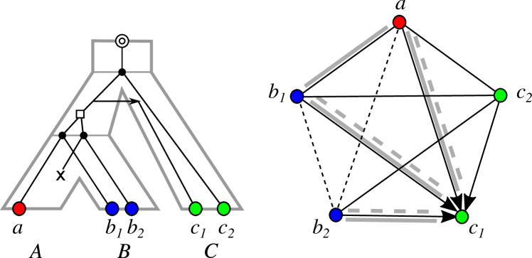
The event-labeled gene tree determines the homology relations (right). The orthology relation comprises all pairs of genes that are connected by a thin solid black edge (without arrows) and correspond to pairs of distinctly colored genes whose last common ancestor is a speciation event. The paralogy relation comprises all pairs of genes that are connected by a thin dashed black edge and correspond to pairs of genes whose last common ancestor is a duplication event. The Fitch (xenology) relation comprises pairs of genes that are connected by thin black arrow-edges. The later-divergence-time relation comprises pairs of genes whose divergence time is below the divergence time of the corresponding species (dashed gray lines) and the reciprocal best match relation comprises all pairs of genes from distinct species and , respectively, for which there is no closer relative for and for (solid gray lines).
Evolutionary scenarios define event types that annotate vertices in gene phylogenies e.g. as speciation or duplication and edges as horizontal transfer. These scenarios in turn form the basis for the formal definitions for the different homology relations among genes such as orthology, paralogy, or xenology Fitch:70 ; Fitch:00 ; Darby:17 , see Fig. 1 for an illustrative example. These three homology relations are not the only relations of interest, however. The (reciprocal) best match relation describes all gene pairs from distinct species that are evolutionary most closely related Geiss:20b ; Geiss:20a ; Stadler2020 ; Geiss+2019 . In contrast to orthology and paralogy, whose definition depends on whether the last common ancestor was a speciation or gene duplication event, it is possible to estimate best matches directly from genomic sequence data. Similarly, the later-divergence-time (LDT) relation comprising gene-pairs that have diverged only after the divergence of the two species in which the genes reside Novichkov:04 ; Schaller:21f ; SHL+23 is informative about the xenology relation, which records whether or not two genes are separated by a HGT event in their evolutionary history. While xenology cannot be measured directed, the LDT relation is accessible from practical data analysis.
The problem of reconstructing a gene family history can be approached in different ways. Tree-based methods start with inferring the gene tree and the species tree separately using well-established phylogenetic methods. This leaves the problem of computing the reconciliation map as a separate optimization problem, typically minimizing the number of loss and HGT events. A problematic issue with this approach is that it crucially depends on accurate tree reconstructions. However, it is difficult to obtain reliable gene trees in particular for gene families with complicated histories Doyle:15 . One remedy is to jointly infer gene trees and species trees, see e.g. BSD+13 ; Szollosi:15 . An alternative approach are tree-free approaches, that estimate binary relations such as reciprocal best matches directly from sequence similarity data and then further analyze these relations to extract orthology and paralogy relations without explicitly constructing trees. It appears that there is no fundamental difference in the accuracy of present-day tree-based and tree-free approaches Altenhoff:09 ; Altenhoff:19 . Methods to infer HGT, reviewed in Ravenhall:15 , fall into three major categories: (1) tree-based approaches that compute an optimal reconciliation w.r.t. some cost function Tofigh:11 ; Chen:12 ; Ma:18 , parametric methods that use genomic signatures, i.e., sequence features specific to a (group of) species identify horizontally inserted material Dufraigne:05 ; Becq:10 , and so-called implicit or indirect methods use distances between genes that are very small or very large compared to the evolutionary distances of the respective species as indicators of HGT Novichkov:04 ; Kanhere:09 . In fact, these methods in essence estimate the LDT relation Schaller:21f .
The purpose of this chapter is to give an introduction into the formal framework of evolutionary scenarios and to review some key mathematical results describing the relationships between binary relations that can be measured from similarity data and the homology relation that are of interest in evolutionary biology. Moreover, we will be concerned with the question how much, and which, information on the gene family history is actually encoded in these binary relations. We shall see that robust estimates of these binary relations already put tight constraints on gene trees, species trees, and reconciliations.
2 Scenarios
2.1 Notation
Graphs are tuples consisting of a vertex set and edge set . Graphs might be undirected (edges are 2-elementary subsets of ) or directed (edges are subsets of ). All graphs considered in this contribution are loop-free, i.e., if or is an edge, then . For a directed graph we write for its underlying undirected graph with . In general, we use the term “graph” for undirected graphs and, otherwise, explicitly write “directed graph”. Moreover, we use the simplified notation for edges in undirected graphs or for the case that both and are edges in a directed graph. Identifying undirected graphs with symmetric directed graphs, furthermore, allows us to make use of subgraph relationships between directed and undirected graphs. We extensively make use of graphs equipped with a vertex-coloring . We say that is properly colored if for all adjacent vertices and .
Rooted Trees naturally describe the phylogenetic relationships both among genes and among species. A rooted tree with vertex set and edge set contains a unique vertex , called the root, that designates the earliest state under consideration. Every path in that originates in thus implies a temporal order and determines the ancestor-descendant relationship as follows: If lies on the unique path from the root to then is an ancestor of , and is a descendant of . In this case we write . For the edges of we write and use the convention that . For an edge , we say that is the parent of and is a child of . It will be useful to extend the ancestor relation to . For a vertex and an edge we set if and only if ; and if and only if . In addition, for edges and in we put if and only if . As usual, is equivalent to or for all . If neither nor holds, we say that and are -incomparable. Note that the root of is the unique -maximal vertex.
The set of all minimal vertices form the leaves of . The subtree rooted at is defined as the subgraph induced by the vertex set . For any subset , the least common ancestor is the -minimal vertex that is an ancestor of all . In particular, we have for all . For simplicity, we write instead of . In addition, we may use the subscript “T” to indicate that is take w.r.t. the tree . Moreover, we set and note that if and only if the root has at least two children. The set of inner vertices of comprise and excludes the root if . A rooted tree is phylogenetic if all its inner vertices have at least two children, and binary if all its inner vertices have exactly two children. We will assume throughout that is phylogenetic but not necessarily binary.
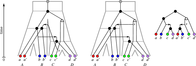
A refinement of a phylogenetic tree is a phylogenetic tree on the same leaf set such that can be obtained from by contracting edges. The restriction of to is the phylogenetic tree with leaf set obtained from the tree by deleting all vertices in and their incident edges and by additionally suppressing all inner vertices of degree two except the root. A phylogenetic tree on some subset is said to be displayed by (or equivalently that displays ) if coincides with , see Fig. 2.
![[Uncaptioned image]](https://cdn.awesomepapers.org/papers/65871071-6f98-4928-a543-5f22d8a841a5/x2.png)
|
|
Rooted triples are binary rooted tree on three vertices. The rooted triple with leaf set and will be denoted by . Triples often can be derived directly from sequence data and reflect the fact that the taxa and are evolutionary closer related than compared to . Hence, it is of interest to determine as whether a given set of triples is consistent, i.e., there is a tree that displays all of the triples in . Aho et al. Aho:81 devised a polynomial-time algorithm, called BUILD, that either constructs a uniquely defined rooted tree that displays or recognizes that is inconsistent. In some situations we also may have information about triples that are not displayed by the tree of interest. A pair of two triple sets is consistent if there is a tree that displays all of the triples in but none of the triples in . The polynomial-time algorithm MTT (“mixed triplets problem restricted to trees”) He:06 tests consistency of pairs of triple sets in polynomial time.
Planted trees. Evolutionary events of interest may also pre-date the last common ancestor of all species or genes. The latter can be accommodated by considering planted trees, i.e., trees that satisfy . In this case is also called the planted root. In a planted phylogenetic tree, and are connected by the edge . The planted root can be thought of a representing the “outgroup(s)”, while represents the “in-group”, i.e., the species or genes under consideration. A planted tree always displays the rooted tree obtained by contracting the edge .
Dated Trees. With each (planted) tree we can associate a time map such that implies . It is an easy task to verify that, for every tree, such a time map exists. Even more, for every tree one can construct, in linear-time, a time map such that leaves of the tree are assigned to particular time-points (e.g. all leaves are mapped to the time-point specifying extant taxa nowadays) SHL+23 . It is usually difficult and often impossible to obtain reliable, accurate “time stamps” for evolutionary relevant events Rutschmann:06 ; Sauquet:13 . Such detailed information is not needed for our purposes. The theoretical results will depend only on the existence of relative timing, i.e., the knowledge as whether an event pre-dates, post-dates, or is concurrent with another one; an information that is often much easier to extract from data Ford:09 ; Szollosi:22 .
Throughout this chapter we assume that all trees are planted and phylogenetic, unless explicitly stated otherwise.
2.2 Reconciliation
Genes evolve within genomes, i.e., species. In order to understand the relationship between genes and species, we need to describe how the gene tree “fits together” with the species tree . This idea is formalized by the notion of a reconciliation map that locates the vertices of the gene tree, i.e., the evolutionary events in the history of the genes, in the species tree. We model evolutionary events as precise point in time. This is, of course, an approximation. In reality, even punctual events such as gene duplications require time to spread through a population and become fixed. Similarly, speciation is also a population-based process that takes time Marques:19 and may also involve additional effects such as incomplete lineage sorting Zheng:14 ; Chan:17 . Nevertheless, it is justified to view events as points-in-time in the context of macro-evolutions, where population effects are neglected altogether.
In order to study reconciliation from a formal point of view, we start out with only minimal requirements that are straightforward to argue:
Definition 1
Let and be trees. A reconciliation of and is a triple where is a map that satisfies the following conditions:
-
(R0)
if and only if
-
(R1)
if and only if
-
(R2)
If and , then
-
(R3)
If , then
While Condition (R0) is used to identify the planted roots, Condition (R1) ensures that leaves of , i.e., extant genes, are found in leaves of , i.e., in extant species. Condition (R2) ensures that temporally distinct speciation events cannot be mapped to the same vertex in , i.e., the same speciation event. Condition (R3), finally ensures a weak form of temporal consistency by forbidding that a descendant of in can be mapped to an ancestor of in . Thus, if , then either or and are -incomparable. For completeness we note that many authors prefer reconciliation maps of the form , i.e., mappings from vertices to vertices Tofigh:11 ; Bansal:12 ; Stolzer:12 . This can be easily translated, however: If , then , i.e., everything is mapped to the lower end of the edge in . The other direction is a bit more intricate. In essence, however, it suffices to set if and there is a with .
An important distinction in evolution is the difference between vertical and horizontal inheritance. Vertical inheritance implies that the the descendants of a gene are harbored by descendant species. In contrast, horizontal inheritance, i.e., horizontal transfer consists in the relocation of a gene to a different lineage. Formally, this situation can be captured by distinguishing vertical and Horizontal Gene Transfer (HGT) edges in the gene tree :
Definition 2
Let be a reconciliation. An edge is an HGT-edge if and are -incomparable. A reconciliation is HGT-free if and are -comparable for all .
As a direct consequence of (R3), a reconciliation is HGT-free if and only if it satisfies
-
(R4)
If then .
In fact, (R4) states that all edges of correspond to vertical inheritance.
Usually, it is known a priori which gene is found in which species. That is, a map is given that assigns to each extant gene the extant species in which it occurs.
Definition 3
Let and be two trees and . Then is a -reconciliation if is a reconciliation and satisfies .
An early important observation in this field is that every gene tree can be reconciled with any species tree even without the need to consider horizontal gene transfer Guigo:96 ; Page:97 :
Theorem 2.1
For any two trees and and any map there is a HGT-free -reconciliation .
To see this, it suffices to consider the reconciliation map defined by setting
| (1) |
![[Uncaptioned image]](https://cdn.awesomepapers.org/papers/65871071-6f98-4928-a543-5f22d8a841a5/x3.png)
|
|
Every reconciliation map can be used to imply gene loss events. To see this, consider an edge such that for a given reconciliation map and for which there is a vertex with , and thus . During the speciation , a descendant of the each gene present in the genome is transmitted to every descendant lineage, i.e., to every edge . If no descendant of the gene is found in a species descending from , then the gene must have died out in the entire species subtree . This is explained most parsimoniously by a single loss event occurring already along the edge . Fig. 3 shows that for the case of the reconciliation this reasoning implies an unrealistically large number of gene loss events: for example, the five paralogs present at the earliest speciation give rise to a total of 10 genes, of which half are subsequently lost again. This reconciliation will in general not be a plausible biological explanation because it implies unreasonably large number of gene losses. This observation led to the development of a number of alternative scoring functions for reconciliation maps with given trees and and a given leaf assignment that count the number of duplication and/or gene losses. We refer to Zhang:97 and the references therein for detailed discussion.
We briefly consider this optimization problem for the HGT-free case here. Assume that we are given a leaf-assignment . The task is then to find a -reconciliation that optimizes a given scoring function. By Thm. 2.1 we know that a solution always exists. Since any vertex has to be mapped at or above the last common ancestor of all the species in which the descendants of are found, every solution satisfies
| (2) |
The so-called LCA reconciliation attains equality whenever possible. More precisely, we define as follows. For each , let and be the parent of in which always exists in planted trees.
The LCA-reconciliation is the most parsimonious reconciliation w.r.t. to several cost measures including the number of duplications and the number duplications and gene losses Chen:00 ; Zhang:97 ; Zmasek:01 . Corresponding maximum likelihood and Bayesian methods is described in Gorecki:11 and Arvestad:03 , respectively. Most parsimonious reconciliations can still be computed in polynomial time if HGT events are included and penalized Bansal:12 ; Tofigh:11 . However, as we shall see in the following section, these reconciliations are not always biologically feasible, see also Menet:22 .
2.3 Relaxed Scenarios
It was noted in Bansal:12 ; Tofigh:11 that the definition of reconciliations in the previous section is not sufficient to ensure that can be interpreted as series of events along a linear time axis. To this end we consider evolutionary scenarios as reconciliations of dated trees:
Definition 4
A (relaxed) scenario consists of a dated gene tree , a dated species tree , and a reconciliation map such that
-
(S0)
if and only if ,
-
(S1)
if and only if ,
-
(S2)
for all with , and
-
(S3)
for all with .
Axioms (S0) and (S1) coincide with (R0) and (R1), respectively, in the definition of a reconciliation. The remaining two axioms, (S2) and (S3), specify time consistency. As for reconciliations in the previous section, we do not assume that a leaf-map is given, although this typically will be the case in practical applications.
Definition 5
A tuple is is a relaxed -scenario if is a relaxed scenario and satisfies .
Relaxed scenarios can be seen as reconciliations for which a time axis is given explicitly. It is not difficult to show that for a given a relaxed scenario , the triple is indeed a reconciliation (cf. Lemma 2 and 3 in SHL+23 ). The converse, however, is not true in general, i.e., it is not always possible to find time stamps that turn a reconciliation into a relaxed scenario cf. e.g. Fig. 2 in Nojgaard:18a . This motivates the following
Definition 6
A reconciliation is time consistent if there are dating maps and such that is a relaxed scenario.
A variety of different auxiliary graphs on Tofigh:11 ; Stolzer:12 or Nojgaard:18a ; Lafond:20 were introduced to summarize the temporal constraints. In each case, it was shown that a reconciliation is time consistent if and only if the corresponding auxiliary graph is acyclic. It can be shown, furthermore, that these auxiliary graphs are acyclic in the special case of HGT-free reconciliations, i.e., every HGT-free reconciliation is automatically time-consistent and can be extended to a relaxed scenario.
In the general case, the additional requirement of time-consistency also makes the computation of maximum parsimony reconciliations difficult. As shown in Tofigh:11 , the problem then becomes NP hard.
2.4 Event-Labels
From a biological point of view, the inner vertices of the gene tree model evolutionary events. In the case of HGT-free scenarios, i.e., reconciliations that satisfy (R4), there are only two fundamentally distinct events: gene duplications and speciation events. Since speciation events are also modeled by the inner vertices , it is natural to distinguish duplications and speciation by their image under the reconciliation map . This naturally leads to the following definition Geiss:20b :
Definition 7
Let be a HGT-free reconciliation. Then the event labeling on is the map given by:
The first two cases, and , distinguish the planted root and the leaves of . The remaining two cases identify speciation events with the that are mapped to inner vertices in the species tree. In contrast, if , it does not correspond to a speciation and thus corresponds to a gene duplication, denoted by . The conditions on the reconciliation considered so far, however, are not sufficient to ensure that with represents a biologically meaningful speciation event. Additional constraint on the evolutionary scenario need to be introduced.
This is possibly best explained by assuming to have a binary gene tree . In this case, if , the two children and of should be mapped via into two distinct lineages. Otherwise, if and are mapped into the same lineage there is no clear historical trace that justifies to be a speciation vertex. In other words, is biologically plausible, if for the two children and of the images and are -incomparable. Moreover, similar to Eq. 2 and to accommodate most parsimonious reconciliation (LCA-reconciliation) one may assume that . The latter discussion naturally translates to the case of general not necessarily binary gene trees as follows:
-
(R5)
Suppose for some . Then
-
(i)
for at least two distinct children of in .
-
(ii)
and are incomparable in for any two distinct children and of in .
-
(i)
As shown in Geiss:20b ; Nojgaard:18a , the axioms (R0)-(R5) are equivalent to axioms that are commonly used in the literature Gorecki:06 ; Vernot:08 ; Doyon:11 ; Rusin:14 ; Hellmuth:17 . In particular, for any HGT-free -reconciliation , there is a LCA-reconciliation for and Hellmuth:17 . The latter observation can easily be extended for -reconciliations involving HGTs and by considering LCA-maps restricted to the HGT-free subtrees of Hellmuth:17 . Thus, the axiom set used here naturally corresponds to LCA-mappings and hence, to most parsimonious reconciliations. In addition, (Geiss:20b, , Lem.2) shows that for a pair of distinct children and of implies for all HGT-free -reconciliations that satisfy (R5). This is turn motivates to consider the extremal event labeling , which assume that these are the only duplications and thus assigns whenever for all pairs of children of . It is important to note that the extremal labeling is defined solely on the information of and does not depend on the existence of a species tree or a reconciliation map .There is no a priori guarantee, therefore, that the extremal event labeling can be realized by an actual biological scenario.
3 Best Match Graphs and Orthology
3.1 Definition and Characterization
Many of the combinatorial methods for determining orthology start from reciprocal best (blast) hits. Here, we consider best matches as a basic evolutionary concept that is approximated on sequence data by “best hits”. We therefore consider best matches relative to an underlying phylogenetic tree, albeit this tree is usually unknown. Our starting point is therefore a gene tree together with a map , where is a set of species. It will be convenient to treat as a coloring of the leaves of tree by the species in which the extant genes reside.
Definition 8
Let be a leaf-colored tree. A leaf is a best match of the leaf if and holds for all leaves from species . The leaves are reciprocal best matches if is a best match for and is a best match for .
Note that a gene may have two or more (reciprocal) best matches of the same color . Some orthology detection tools, such as ProteinOrtho Lechner:11a , explicitly attempt to extract all reciprocal best matches from the sequence data.
A directed, vertex-labeled graph is a best match graph (BMG) if there is a leaf-labeled tree such that is a directed edge in if and only if is best match of in . Given we write for its best match graph.
A key observation towards characterizing best match graphs is that some subsets of vertices on two colors (species) yield constraints on triples displayed by any leaf-colored tree that might explain a BMG.
Definition 9
Let be pairwise distinct vertices in a colored digraph such that and . Then the triple is informative if and forbidden if .
The sets and denotes the set of all informative and forbidden triples, respectively. It is shown in Geiss:20b that, if , then displays all triples in and none of the triples in . The sets and also give rise to convenient characterizations of BMGs.
Theorem 1
A properly colored digraph is a BMG if and only if one of the following conditions is satisfied.
-
(i)
is consistent and Geiss:20b ; Schaller:21d
-
(ii)
is consistent and is color-sinkfree, i.e., for every and every color there is a vertex such that and with . Schaller:21b
In particular, BMGs be be recognized in polynomial-time.
Intriguingly, every BMG is associated with a unique least-resolved tree . That is, (i) and (ii) if then displays . The least resolved tree therefore captures the reliable phylogenetic information about the gene tree that is provided by the best matches. The least-resolved tree for a BMG is precisely the tree and can be constructed in polynomial time.
While least-resolved trees serve as a scaffold to cover phylogenetic information without making more assumptions on the evolutionary history than actually provided by the data, one is in many cases additionally interested to find binary trees which can be considered as the most “highly” resolved histories. Binary trees are of particular interest because true multifurcations are most likely rare, i.e., most polytomies are a consequence of insufficient resolution of the available data Maddison:89 ; DeSalle:94 ; Walsh:99 . However, not every BMG can be explained by a binary tree (cf. (Schaller:21a, , Fig.6A)). Binary explainable BMGs are characterized as those BMGs that do not contain a certain colored graph on four vertices, termed hourglass, as induced subgraph Schaller:21a . Note that binary trees explaining a BMG are not necessarily unique, however, they all display and can be constructed in polynomial time Schaller:21e .
Binary explainable BMGs also have a convenient characterization in terms of triple sets. Consider the following extension of the set of informative triples:
| (3) |
As shown in Schaller:21e , replacing by in Thm. 1 yields a characterization of binary explainable BMGs. Moreover, if is a binary explainable BMG, then has the property that a binary tree satisfies if and only if is a refinement of . We summarize these results in the following
Theorem 2
The following statements are equivalent for every BMG :
-
(i)
is binary explainable.
-
(ii)
is hourglass-free Schaller:21a .
-
(iii)
is consistent Schaller:21e .
In this case, a binary tree that explains can be constructed in polynomial time. In particular, the BMG is explained by every refinement of the tree Schaller:21e .
In practice, is obtained empirically by comparing similarities of gene sequences. Most likely, thus will not be a BMG but differ from the true best match graph by both false positive and false negative edges. The arc modification problems for BMGs aim at correcting such errors. Like most graph editing problems, it is NP-complete Schaller:21b ; Schaller:21e . However, efficient heuristics can be devised that solve the problem with acceptable accuracy Schaller:21g
3.2 Orthology in the Absence of HGT
Walter Fitch Fitch:70 defined orthology as homology deriving from a speciation event. While later discussions qualified this simple concept in the presence of HGT (see below), the notion is clear in a HGT-free setting. We assume throughout this section that scenarios and reconciliations are HGT-free.
Definition 10
Let be an event-labeled gene tree and let be two distinct genes. Then and are orthologs if ; they are paralogs if .
We write for the orthology graph with vertex set and edges whenever and are orthologs. Note that the corresponding “paralogy graph” is simply the complement graph of . Moreover, is symmetric but not necessarily transitive (edges and do not imply that is an edge). Orthology graphs feature a simple structure:
Theorem 3 (Hellmuth:13a )
A graph is an orthology graph for some event-labeled tree , i.e. , if and only if is a cograph.
A classical characterization of cographs is the following: is a cograph if and only if it does not contain a , i.e, a path on four vertices, as an induced subgraph Corneil:81 .
Given a reconciliation , orthology is therefore implied by the reconciliation maps, since, by Def. 7 above, specifies the event labeling . The dependence of orthology on is crucial. In the extreme case of , we have , and thus all events are classified as duplications. Conversely, the LCA reconciliation maps as many to inner vertices of as possible, and thus can be expected to result in a large number orthologous pairs.
The starting point for many algorithmic approaches to orthology detection is the observation that two orthologs and are also reciprocal best matches. We are therefore in particular interested in obtaining information on the orthology relation starting from best match data only.
Writing for the subgraph of the best match comprising the reciprocal, i.e., bi-directional edges, and denoting by the extremal event labeling for introduced in the previous section, we obtain the following key result:
Theorem 4 (Geiss:20b )
Let be a HGT-free -reconciliation satisfying (R5). Then .
Theorem 4, in particular, shows that using the reciprocal best match graph as an approximation for the orthology relation does not yield false negative orthology assignments. In general, however, is a proper subgraph of , i.e., reciprocal best match graphs may contain false-positive orthology assignments. In particular, does not need to be a cograph and thus may contain induced s.
If for some children and of then for all HGT-free -reconciliations that satisfy (R5) (cf. (Geiss:20b, , Lem.2)). (Schaller:21a, , Lemma 10) characterizes false orthology assignments in best matches graphs and provides an even stronger results. In particular, it shows that precisely if for some children and of . Using the fact that allows us to rephrase this result in following, more convenient form:
Theorem 5
The following statements are equivalent for every tree and any two leaves and of .
-
(i)
and are paralogs in any HGT-free -reconciliation
-
(ii)
There are two children and of such that .
-
(iii)
are “false orthologs” in case and are reciprocal best matches.
Note that Thm. 5 depends on the structure of the underlying tree and trees that explain a given BMG are not necessarily unique. Hence, there might be a tree such that but for which an edge is a false-positive orthology assignment w.r.t. but not w.r.t. . Hence, we are interested, in particular, in those bi-directional edges of a BMG that are false orthology assignment for every tree that satisfies . Such edges are called unambiguously false orthology assignment in and can be identified in chains of overlapping hourglasses. For the details we refer to Def.14 and Def.16 in Schaller:21a for the detailed specification of all “hug”-pairs and we obtain
Theorem 6 ((Schaller:21a, , Thm.11 & 12))
An edge in a BMG is an unambiguously false orthology assignment if and only and is a “hug”-pair. The set of all unambiguously false orthology assignment in a BMG can be computed in polynomial time.
The no-hug graph is the subgraph of from which all edges that are hug pairs have been removed. In particular, contains the orthology graph for every HGT-free -reconciliation satisfying (R5) as a subgraph (cf. (Schaller:21a, , Cor. 5)):
| (4) |
As shown in Schaller:21a , is in fact an orthology graph. However, since only unambiguously false orthology have been removed, may still contain false orthologs. That is, reciprocal best matches might be paralogs in the true scenario but appear as orthologs in alternative scenarios that are consistent with the best match data. In fact, it is always possible to “move up” a speciation event and to replace it by a duplication followed by losses. In this manner it is always possible to explain best match without orthologs. The no-hug graphs thus provides the “most parsimonious” explanation in the sense that it predicts an orthology relationship whenever this is consistent with the best match data instead of an alternative explanation, which would comprise a duplication event accompanied by complementary losses. Thus, the reconciliation underlying is a least conceptually related to LCA reconciliations. A closer inspection of this connection, however, is a topic for future research.
In practice, one could obtain an accurate orthology assignment by estimating an initial, species labeled graph representing best (blast) hit data and then edit these initial data to a BMG, i.e., a graph that conforms to Def. 8. This step is, in general, NP-hard HGS:20 ; Schaller:21b and thus, will require an efficient heuristic. From the the BMG we can then remove, in polynomial-time, all hug-pairs to obtain the no-hug graph that is free of unambiguously false orthologs and also an orthology graph.
Since orthology graphs are cographs, there is also a more direct, albeit less accurate approach towards estimating the orthology graph. To this end, one extracts the reciprocal best hits from the initial estimated best (blast) hits and finds the cograph that differs by the fewest edge-insertions and edge-deletions from . This cograph editing problem is also NP-hard Liu:12 . However, it remains tractable if is not too dissimilar from a cograph. Fast heuristics have become available for this task in last years White:18 ; Hellmuth:20b ; Crespelle:21 .
By Theorem 1, BMGs can be recognized in polynomial-time and the tree is the unique least resolved tree that explains a BMG . However, it is not possible in general to equip with an event labeling such that . Instead, can be augmented to a uniquely defined tree that is equipped with the extremal event labeling . The event labeled tree satisfied
| (5) |
and can be obtained in polynomial time (cf. (Schaller:21a, , Thm.10)). The extremal labeling is defined solely on the information of and does not depend on the existence of a species tree or a reconciliation map .
In summary, therefore, it is possible to use the information of a BMG to get mathematically sound estimates of orthology relations and a resulting gene tree such that in polynomial time.
An intriguing observation is that the event labeled gene trees have implications for the species tree irrespective of the details of the reconciliation map. To this end, let denote the set of all triples that satisfy (i) , , and are pairwise distinct species and (ii) , i.e., the root of is a speciation event.
Proposition 1 (HernandezRosales:12a ; Hellmuth:17 )
For a given event-labeled tree and species map the following two statements are equivalent.
-
(i)
There is a species tree such that there is a HGT-free -reconciliation with .
-
(ii)
The triple set is consistent.
Note that the set of species triples in Prop. 1 depends on the event-labeling of , but not on the details of the reconciliation map as long as gives rise to correct event-labeling. Several types of problems that are concerned with optimally editing a given undirected graph to an orthology relation that, at the same time, satisfies additional constraints (e.g. that the resulting event-labeled gene tree can be reconciled with some (unknown) species tree) have been considered e.g. in Lafond:16 . While most of the latter problems are NP-complete, certain types of problems that are related to the correction of homology relations that provide only partial information about orthologs and non-orthologs can be solved in polynomial-time Lafond:14 ; Nojgaard:18b .
Although Prop. 1 is rather technical, it has significant practical importance. An estimate of , e.g. obtained directly from reciprocal best match data by means of cograph editing provides a collection of species triples. Pooling these data over a large number of gene families indeed yields sufficient information to infer fully resolved species trees Hellmuth:15a .
3.3 Clusters of Orthologous Genes
Orthologs are often summarized as clusters of orthologous groups (COGs) Tatusov:97 . We have seen, however, that orthologous genes form cographs, and hence orthology is in general not a transitive relation. COGs are only an approximation that is particularly useful if the the gene family history contains only a small number of duplications. A special case is one-to-one orthology, where each gene has a unique ortholog in every other species. In this case, the orthology relation becomes transitive and the the orthology graph reduces to a disjoint union of cliques Roth:08 . These clusters, e.g. computed by OMA Roth:08 , are induced complete subgraphs, i.e., cliques in the full orthology graph.
Most other approaches to computing COGs allow co-orthologs, i.e., clusters are not restricted to cliques of the orthology graph and thus, may include orthologs and paralogs Tatusov:97 . A wide variety of clustering algorithms have been used to extract COGs from sequence similarity data. The definition of such COGs necessarily depends on stringency parameters that gauge the trade-off between size and stringency of COGs. From a theoretical point of view transitivity clustering Rahmann:07 is interesting because of its conceptual similarity to co-graph editing: here the initial orthology estimate is edited by insertion end deletion of edges to a transitive graph, i.e., a partitioning into COGs. In Falls:08 , maximal Túran (complete multipartite) graphs are computed. These form a special class of co-graphs and accommodate so-called in-paralogs TremblaySavard:12 ; Altenhoff:19 , i.e., duplicate gene that originated after the most recent speciation event in each lineage. Complementarily, it is of interest to partition a gene set such that out-paralogs (i.e., pairs of genes arising from duplications that pre-date all speciation events) are placed in different clusters. These correspond to the connected components of the orthology graph .
4 Fitch Graphs and Horizontal Gene Transfer
4.1 Definition and Characterization
Fitch Fitch:00 defined “two genes and as xenologs if their history, since their common ancestor, involves an interspecies (horizontal) transfer of the genetic material for at least one of them.” Two leaves in in a tree are thus xenologs whenever the unique path connecting and in contains an HGT-edge. By Def. 2, the subset of HGT-edges , and thus xenology, depends explicitly on the reconciliation . As in the previous sections, we are interested in inferring xenology without first computing a reconciliation . Again, we approach this problem by studying properties of graphs that are implied by reconciliation or a relaxed scenario.
Let use first consider the parts of a scenario that are unaffected by HGT events. Deleting from all HGT-edges yields a forest and induces a partition of of the leaf set such that the restriction contains no HGT-edges. Consequently, one can perform the analysis of HGT-free systems outlined above for each of the gene sets separately. Note that in general, this does not amount to simply considering the subgraph of empirical BMGs induced by . In general the empirical BMGs with will feature best matches that might be worse than those best matches in that are implied by and the additional knowledge of HGT-edges. We shall return to the inference of HGT-edges and the partitioning of the gene set into maximal HGT-free subsets below.
Mechanistically HGT is a inherently directional event. There is a clear distinction between the horizontally transferred ”copy” and the “original” that continues to be transferred vertically. It is significant, therefore, whether HGT-edges are found along the path from to , the path from to , or along both paths. Mathematically, this can be captured in the following manner.
Definition 11
Let be a rooted tree and be a set of HGT-edges. Then the (directed) Fitch graph has vertex set and if the path from to contains an edge .
A graph is a (directed) Fitch graph if for some tree and edge set . In Geiss:18 a characterization of Fitch graphs in terms of eight forbidden subgraphs on three vertices is given.
Fitch graphs also have a surprisingly simple characterization in terms of their “closed complementary neighborhoods”. For a directed graph consider
| (6) |
Since all graphs considered here are loop-free, we have . We write .
Theorem 7 (HS:19 )
is a Fitch graph if and only if (i) is hierarchy-like, i.e., for hold , and (ii) for every and every holds .
If is a Fitch graph, then , i.e., the extension of the closed complementary neighborhoods by the singleton sets and itself forms a hierarchy on , which corresponds to a uniquely defined rooted tree . This tree is the unique least-resolved tree for and the set of HGT-edges in is uniquely determined and consists of all edges in with HS:19 ; Geiss:18 . The directed Fitch graph thus is also informative about the structure of the gene tree. The pair also immediately yields the partition of into HGT-free subsets.
The symmetric version of a directed Fitch graph , called undirected Fitch graph, contains all bi-directional edges . Thus, if and only if the path between and contains a HGT-edge. Undirected Fitch graphs have been studied in HLGS:18 and coincide with the complete multipartite graphs. Hence, undirected Fitch graphs are completely defined by their independent sets. This implies that undirected Fitch graphs cannot convey much interesting phylogenetic information because they are completely determined by the maximal subsets of taxa that have not experienced any horizontal transfer events among them.
The problem of finding a common gene tree from which a given orthology graph and Fitch graph can be derived has been considered in Hellmuth:21b . Moreover, given a leaf-labeled tree and HGT-edges , a result similar in spirit to Prop. 1 determines a set triples that must be displayed the species tree in any -reconciliation that satisfies (R4), (R5), and Hellmuth:17 ; Nojgaard:18a . In Lafond:20 , a polynomial-time algorithm is provided that takes and as input and constructs the species tree and a time-consistent reconciliation map , if one exists.
4.2 LDT Graphs
Unfortunately, no practical way to infer the Fitch graph directly from sequence data has become available so far. A promising approach starts from the observation that if two genes and are more closely related than the species and , then and must be xenologs Novichkov:04 . A statistical sound method for identifying such pairs of genes is described in Kanhere:09 . Although such indirect methods have been quite successful, see Ravenhall:15 for a review, their mathematical properties have been studied only very recently:
Definition 12 (Schaller:21f )
Let and be two dates trees and . Then the undirected graph has vertex set and is an edge if .
A vertex-colored graph is a later-divergence-time graph (LDT graph) if there is a tuple of dated trees and and a map such that . LDT graphs have a simple characterization. To this end, consider the set of rooted triples where , , and are pairwise distinct, and .
Theorem 4.1 (Schaller:21f )
A graph is an LDT graph if and only if it is properly colored cograph and the triple set is compatible.
A polynomial time algorithm to construct a relaxed -scenario for a given LDT graph is also described in Schaller:21f . Not surprisingly, the editing problem for LDT-graphs is NP-complete.
An LDT-graph is always a subgraph of the undirected Fitch graph for any relaxed -scenario that satisfies . Thus, LDT graphs cannot contain false-negative xenologous gene-pairs, and the complement of an LDT graph contains in particular all edges between pairs of genes that are not separated by a HGT event. In order to apply methods developed for HGT-free data, we need to find the partition into maximal HGT-free subsets of a given sets of genes . In practice, this can be done by using the solution of the so-called cluster deletion problem applied on , i.e., of deleting a minimum set of edges from such that the resulting graph is a disjoint union of complete graphs Shamir:04 . Defining as the vertex set of the -th clique in then yields the desired partition of into maximal HGT-free subsets. If (or equivalently ) is a cograph, cluster deletion can be solved in linear time by a greedy algorithm Gao:13 . The LDT graph thus can be used to obtain a the partition of into HGT-free subsets. Compatibility of such partitions with a given gene tree as well as inferring the directions of HGT-edges using such partitions have been the topic in HSS:22 ; SHS:23
4.3 Orthology in the presence of HGT
Most of the mathematical results concerning orthology have been obtained in an HGT-free setting. In the presence of HGT, descendants of two genes that originate from a speciation event may even eventually reside in the same species, where they appear as paralogs. This has led to different proposals for the “correct” definition of orthology. A classification of subtypes of xenology that, in line with Fitch:00 , reserves the terms ortholog and paralog to situations in which the path between and does not contain an HGT event was proposed in Darby:17 . Similar to LDT graphs, “Equal Divergence Time” (EDT) graphs capture that fact that the divergence time of two genes and matches the divergence time of the species in which they reside. Similar to LDT graphs, a vertex-colored undirected graph is an EDT graph, if there are for two dated trees and and such that precisely if . In this case, we also write . In general, EDT graph recognition is NP-hard SHL+23 , however, it becomes polynomial-time solvable if information of the LDT graph is available. To see this, observe that complementary graph of the union of the EDT and LDT graph contains all edges for which which determines the so-called prior divergence time graph and we can apply (SHL+23, , Cor. 8).
One easily verifies that, in a HGT-free -reconciliation that satisfies (R5), Axiom (R5)(i) implies that two genes and are orthologs if their last common ancestor coincides with the last common ancestor of the two species in which and reside. In this case, there is an obvious connection between orthology and the EDT graphs. We summarize now results that shows that EDT graphs are also closely connected to different notions of orthology in scenarios with HGT that have been discussed in the literature. Disagreements on the definitions of orthology in the presence of HGT stem for the fact that, in general, pairs of genes originating from a speciation event may be separated by HGT, and thus become xenologs. At the same time, they may even eventually reside in the same species and therefore appear as paralogs.
Definition 13
Let be a relaxed -scenario. Then, two distinct vertices are
-
•
weak quasi-orthologs if .
-
•
weak orthologs if and there is no HGT-edge along the path between and in .
-
•
strict quasi-orthologs if .
-
•
strict orthologs if and is no HGT-edge along the path between and in .
The undirected graphs , , , and , resp., have vertex set and edges precisely if the genes and are weak quasi-orthologs, weak orthologs, strict quasi-orthologs, resp., strict orthologs in , see Table 1 for a summary.
| Reconciliation condition | HGT irrelevant | HGT excluded |
|---|---|---|
| weak quasi-ortholog | weak ortholog | |
| strict quasi-ortholog | (strict) ortholog |
Weak quasi-orthologs are, in essence, Walter Fitch’s original, purely event-based definition of orthology Fitch:70 . In later work, Fitch Fitch:00 emphasizes the condition that “the common ancestor lies in the cenancestor (i.e., the most recent common ancestor) of the taxa from which the two sequences were obtained”, which translates to the notion of strict quasi-orthologs. Other definitions of orthology explicitly exclude xenologs Gray:83 ; Fitch:00 ; Darby:17 , which leads the concept of weak and strict orthologs.
As shown in SHL+23 , for every relaxed -scenario , we have
| (7) |
while and are incomparable w.r.t. the subgraph relation. Moreover, the weak quasi-orthology graph , the weak orthology graph and the strict orthology graph are cographs for every relaxed . This is not true in general for the strict quasi-orthology graph . There is a close connection between LDT and EDT graphs and weak and strict orthologs:
Proposition 2
(SHL+23, , Prop. 5) Given two graphs and there is a relaxed -scenario such that and if and only if there is relaxed -scenario with and that in addition satisfies .
That is, a pair of an LDT and EDT graph can be explained by a common relaxed scenario, if there the two graphs can be explained a relaxed scenario for which weak and strict orthology coincide.
In the generic case, unrelated evolutionary events happen at distinct time points:
Definition 14
A relaxed scenario is generic if for and , then .
In generic scenarios, the EDT graph and the different notions of orthology are connected as follows:
| (8) |
In the HGT-free case all these graphs coincide if implies . A full formal understanding of orthology and its variants in the presence of HGT is still lacking, however.
5 Discussion and Open Problems
In this chapter we provided an overview of the current formal, mathematical understanding of gene family histories with a focus on “tree-free” methods. We deliberately excluded full-fledged probabilistic models from our discussion. These also start from the idea of scenarios and use stochastic models of sequence evolution to assign probabilities, which are then used in maximum likelihood or Bayesian setting to reconstruct scenarios Arvestad:03 ; Akerborg:09 ; Larget:10 . While these detailed models promise accurate results for small and medium data sets, it is unclear whether they scale to very large problems. The combinatorial approach outlines here, on the other hand, holds promise to be able to address gene family histories at global scales.
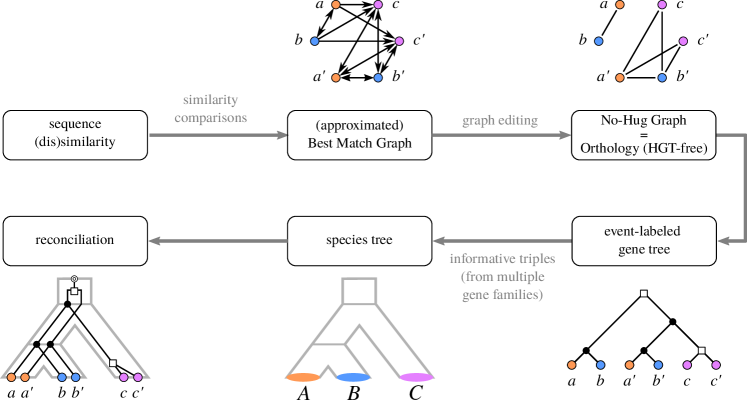
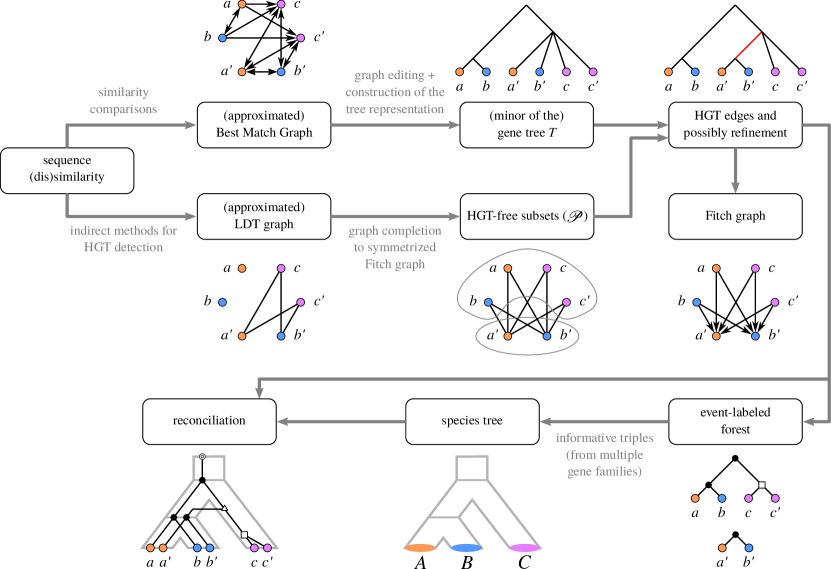
Taken together, Figs. 5 and 6 outline a common conceptual workflow for a comprehensive analysis of gene family histories in a “tree-free” setting. Instead of a gene tree and a species tree , a BMG and LDT/EDT graphs are estimated from the data. Together, these two graphs capture the salient information, as outlined in the formal results in the previous sections. The main advantage of this approach over the direct reconstruction of trees is that it can make use of the inherent redundancies in the data. Following the independent estimate of the edges of the BMG and LDT/EDT graphs, one can use the fact well-formed BMGs and LDT graphs belong to highly restrictive, special graph classed, as means of data correction: the initial estimates can be edited to the closest well-formed graphs of the respective type. Unfortunately, these graph editing problems are NP-complete. However, workable heuristics have already been developed for this purpose. The hardness of this data correction task also does not amount to a conceptual argument against the workflow proposed in Fig. 6; after all, both the multiple sequence alignment problem, see Elias:06 and the references therein, and the reconstruction of a phylogenetic tree by means of maximum parsimony or maximum likelihood are also NP-complete Day:83 ; Day:87 ; Roch:06 . From the BMG and LDT/EDT graphs one can now obtain a not necessary fully resolved gene tree, sufficient information of the species, as well as a corresponding event labeling that located all relevant evolutionary events. In a final step, the resolution of the gene tree and the species could be improved by conventional phylogenetic methods using the combinatorially inferred trees and as constraints. Although the time of writing this chapter no full-fledged implementation have become available, the individual steps have been benchmarked using simulated data and shown to be feasible in a realistic setting Schaller:22a .
The notion of reconciliation generalizes beyond the scope of this chapter, which focuses on genes as part of genomes, or, equivalently host-parasite systems Page:97 ; Merkle:10 . The same structure arises when the evolution of domains in proteins is considered. This naturally gives rise to a multi-level version of reconciliation Menet:22 ; Penel:22 . In addition to speciation, gene duplication, gene loss, and horizontal transfer, it is of interest to consider additional event types. Incomplete lineage sorting or deep coalescence as well as hybridization, in particular, have received considerable attention Stolzer:12 ; Zheng:14 ; Chan:17 ; Du:18 ; Ansarifar:20 . Interestingly, maximum parsimony reconciliation becomes NP-hard in this setting LeMay:21 . Phylogenetic networks are natural generalization of phylogenetic trees HHM:19 ; huson_rupp_scornavacca_2010 . The concept of reconciliation persists in such models. In To:15 ; Scornavacca:17 , for instance, reconciliation of gene trees with a restricted classes of species networks are considered. In The problem of reconciling a gene network (motivated by recombination) with a species tree is investigated in Chan:19 , introducing an analog of the LCA reconciliation that provides a solution for so-called tree-child networks. To our knowledge, these extended models have not been studied so far from a “tree/network-free” perspective that would extend the results reviewed in this chapter.
Despite substantial progress since the first edition of this book Setubal:18a , a number of key questions remain open, in particular in relation to the detection and localization of HGT events. Most importantly, the empirically accessible relations (best matches, lower/equal divergence time) provide independent constraints on the reconciliation and inferred orthology and xenology relations may impose additional conditions. In most cases, at least part of the conditions for the existence of an explaining scenario are expressed in terms of consistence of triple sets. This suggests consider consistency of their union. In general this will lead to the NP-complete problem of determining maximum consistent subset(s) of triple or one of its variants Byrka:10 . A better understanding how conflicting constraints arise, however, may point to a more accurate and possibly computationally more efficient way of handling internal conflicts in the data. Complementarily, it will be of interest to investigate how a trusted species tree could be used for the improvement of initial estimated of best match graphs. The fact that information of this type can be helpful has been demonstrated in a maximum-likelihood framework Morel:20 . An interesting variation on this theme are methods to infer species trees and reconciliation maps from a set of gene trees Morel:22 . It also remains unclear whether for given , , and , there exists a reconciliation with a prescribed set of reconciliation edges . We conjecture that, in analogy with the HGT-free case, the answer is affirmative. More generally, event labelings and their consequences are not full understood for relaxed scenarios. While event labeling are implicitly defined as part of reconciliation maps e.g. in Tofigh:11 ; Bansal:12 ; Stolzer:12 , these definitions also restrict the scenarios to which they pertain, see also Nojgaard:18a ; Lafond:20 .
From a practical point of view, the most pressing issue is the development of more efficient heuristics for the graph-editing problems that naturally arise in any real-life application of the tree-free methods. i.e., in the intermediate step of the workflows outlined in Figs. 5 and 6. For both cographs White:18 ; Hellmuth:20b ; Crespelle:21 and BMGs Schaller:21g signficant progress has been reported in the recent past. Full-fledged bioinformatics pipelines for large-scale applications focus primarily on COGs rather than a more fine grained presentation of gene family histories, making only limited use of the progress in mathematical phylogenetics. In conjunction, with much improved methods for genome-wide alignments Armstrong:20 , improved gene family histories may constitute also an important step towards a comprehensive understanding of genome evolution.
References
- [1] Michael Lynch and John S. Conery. The evolutionary fate and consequences of duplicate genes. Science, 290:1151–1155, 2000.
- [2] Asher D. Cutter and Richard Jovelin. When natural selection gives gene function the cold shoulder. Bioessays, 37(11):1169–1173, 2015.
- [3] H Innan and F Kondrashov. The evolution of gene duplications: classifying and distinguishing between models. Nat Rev Genet, 11:97–108, 2010.
- [4] Adrian M. Altenhoff, Romain A. Studer, Marc Robinson-Rechavi, and Christophe Dessimoz. Resolving the ortholog conjecture: orthologs tend to be weakly, but significantly, more similar in function than paralogs. PLoS Comp. Biol., 8(e1002514), 2012.
- [5] R. A. Studer and M. Robinson-Rechavi. How confident can we be that orthologs are similar, but paralogs differ? Trends in Genetics, 25(210-216), 2009.
- [6] T. Gabaldón and E. V. Koonin. Functional and evolutionary implications of gene orthology. Nat. Rev. Genet., 14(5):360–366, 2013.
- [7] N. L. Nehrt, W. T. Clark, P. Radivojac, and M. W. Hahn. Testing the ortholog conjecture with comparative functional genomic data from mammals. PLoS Comput. Biol., 7(e1002073), 2011.
- [8] Erik Sonnhammer, Toni Gabaldón, Alan Wilter Sousa da Silva, Maria Martin, Marc Robinson-Rechavi, Brigitte Boeckmann, Paul Thomas, Christophe Dessimoz, and the Quest for Orthologs consortium. Big data and other challenges in the quest for orthologs. Bioinformatics, 30(21):2993–2998, 2014.
- [9] Jesús A. Ballesteros and Gustavo Hormiga. A new orthology assessment method for phylogenomic data: Unrooted phylogenetic orthology. Mol. Biol. Evol., 33(8):2117–2134, 2016.
- [10] Walter M Fitch. Distinguishing homologous from analogous proteins. Syst Zool, 19:99–113, 1970.
- [11] Walter M. Fitch. Homology: a personal view on some of the problems. Trends Genet., 16:227–231, 2000.
- [12] Charlotte A Darby, Maureen Stolzer, Patrick J Ropp, Daniel Barker, and Dannie Durand. Xenolog classification. Bioinformatics, 33:640–649, 2017.
- [13] Manuela Geiß, Marcos E. González Laffitte, Alitzel López Sánchez, Dulce I. Valdivia, Marc Hellmuth, Maribel Hernández Rosales, and Peter F. Stadler. Best match graphs and reconciliation of gene trees with species trees. J. Math. Biol., 80:1459–1495, 2020.
- [14] Manuela Geiß, Peter F. Stadler, and Marc Hellmuth. Reciprocal best match graphs. J. Math. Biol., 80:865–953, 2020.
- [15] Peter F. Stadler, Manuela Geiß, David Schaller, Alitzel López Sánchez, Marcos González Laffitte, Dulce I. Valdivia, Marc Hellmuth, and Maribel Hernández Rosales. From pairs of most similar sequences to phylogenetic best matches. Algorithms for Molecular Biology, 15:5, 2020.
- [16] Manuela Geiß, Edgar Chávez, Marcos González Laffitte, Alitzel López Sánchez, Bärbel M. R. Stadler, Dulce I. Valdivia, Marc Hellmuth, Maribel Hernández Rosales, and Peter F. Stadler. Best match graphs. Journal of Mathematical Biology, 78(7):2015–2057, 2019.
- [17] Pavel S Novichkov, Marina V Omelchenko, S Gelfand Mikhail, Andrei A Mironov, Yuri I Wolf, and Eugene V Koonin. Genome-wide molecular clock and horizontal gene transfer in bacterial evolution. J. Bacteriol., 186:6575–6585, 2004.
- [18] David Schaller, Manuel Lafond, Peter F. Stadler, Nicolas Wiesecke, and Marc Hellmuth. Indirect identification of horizontal gene transfer. J. Math. Biol., 83:10, 2021. arXiv 2012.08897.
- [19] David Schaller, Tom Hartmann, Manuel Lafond, Nicolas Wieseke, Marc Hellmuth, and Peter F. Stadler. Relative timing information and orthology in evolutionary scenarios. Technical Report 2212.02201, arXiv, 2023.
- [20] V P Doyle, R E Young, G J Naylor, and J M Brown. Can we identify genes with increased phylogenetic reliability? Syst Biol, 64(5):824–837, 2015.
- [21] B Boussau, G J Szöllősi, L Duret, M Gouy, E Tannier, and V Daubin. Genome-scale coestimation of species and gene trees. Genome Res., 23(2):323–330, 2013.
- [22] Gergely J. Szöllősi, Eric Tannier, Vincent Daubin, and Bastien Boussau. The inference of gene trees with species trees. Syst. Biol., 64:e42–e62, 2015.
- [23] Adrian M. Altenhoff and Christophe Dessimoz. Phylogenetic and functional assessment of orthologs inference projects and methods. PLOS Comp. Biol., 5:e1000262, 2009.
- [24] A. M. Altenhoff, N. M. Glover, and C. Dessimoz. Inferring orthology and paralogy. In Evolutionary Genomics, volume 1910 of Methods in Molecular Biology, pages 149–175. Humana, New York, NY, 2019.
- [25] Matt Ravenhall, Nives Škunca, Florent Lassalle, and Christophe Dessimoz. Inferring horizontal gene transfer. PLoS Comp. Biol., 11:e1004095, 2015.
- [26] Ali Tofigh, Michael Hallett, and Jens Lagergren. Simultaneous identification of duplications and lateral gene transfers. IEEE/ACM Trans. Comp. Biol. Bioinf., 8(2):517–535, 2011.
- [27] Zhi-Zhong Chen, Fei Deng, and Lusheng Wang. Simultaneous identification of duplications losses and lateral gene transfers. IEEE/ACM Trans. Comp. Biol. Bioinf., 9, 2012.
- [28] W Ma, D Smirnov, J Forman, A Schweickart, C. Slocum, S. Srinivasan, and R. Libeskind-Hadas. DTL-RnB: Algorithms and tools for summarizing the space of DTL reconciliations. IEEE/ACM Trans. Comp. Biol. Bioinf., 15:411–421, 2018.
- [29] Christine Dufraigne, Bernard Fertil, Sylvain Lespinats, Alain Giron, and Patrick Deschavanne. Detection and characterization of horizontal transfers in prokaryotes using genomic signature. Nucleic Acids Res., 33:e6, 2005.
- [30] Jennifer Becq, Cécile Churlaud, and Patrick Deschavanne. A benchmark of parametric methods for horizontal transfers detection. PLoS ONE, 5:e9989, 2010.
- [31] Aditi Kanhere and Martin Vingron. Horizontal gene transfers in prokaryotes show differential preferences for metabolic and translational genes. BMC Evol. Biol., 9:9, 2009.
- [32] João C. Setubal and Peter F. Stadler. Gene phylogenies and orthologous groups. In João C. Setubal, Peter F. Stadler, and Jens Stoye, editors, Comparative Genomics, volume 1704, pages 1–28. Springer, Heidelberg, 2018.
- [33] A. V. Aho, Y. Sagiv, T. G. Szymanski, and J. D. Ullman. Inferring a tree from lowest common ancestors with an application to the optimization of relational expressions. SIAM J. Comput., 10:405–421, 1981.
- [34] Ying-Jun He, Trinh N D Huynh, Jesper Jansson, and Wing-Kin Sung. Inferring phylogenetic relationships avoiding forbidden rooted triplets. J. Bioinf. Comp. Biol., 4:59–74, 2006.
- [35] Frank Rutschmann. Molecular dating of phylogenetic trees: A brief review of current methods that estimate divergence times. Diversity and Distributions, 12:35–48, 2006.
- [36] Hervé Sauquet. A practical guide to molecular dating. Comptes Rendus Palevol, 12:355–367, 2013.
- [37] Daniel Ford, Frederick A. Matsen, and Tanja Stadler. A method for investigating relative timing information on phylogenetic trees. Systematic Biology, 58:167–183, 2009.
- [38] Gergely Szöllősi, Sebastian Höhna, Tom A Williams, Dominik Schrempf, Vincent Daubin, and Bastien Boussau. Relative time constraints improve molecular dating. Systematic Biology, 71:797–809, 2022.
- [39] David A Marques, Joana I Meier, and Ole Seehausen. A combinatorial view on speciation and adaptive radiation. Trends Ecol Evol, 34:531–544, 2019.
- [40] Y Zheng and L. Zhang. Effect of incomplete lineage sorting on tree-reconciliation-based inference of gene duplication. IEEE/ACM Trans Comput Biol Bioinform, 11:477–485, 2014.
- [41] Y B Chan, V Ranwez, and C. J. Scornavacca. Inferring incomplete lineage sorting, duplications, transfers and losses with reconciliations. Theor. Biol., 432:1–13, 2017.
- [42] Mukul S. Bansal, Eric J. Alm, and Manolis Kellis. Efficient algorithms for the reconciliation problem with gene duplication, horizontal transfer and loss. Bioinformatics, 28:i283–i291, 2012.
- [43] Maureen Stolzer, Han Lai, Minli Xu, Deepa Sathaye, Benjamin Vernot, and Dannie Durand. Inferring duplications, losses, transfers and incomplete lineage sorting with nonbinary species trees. Bioinformatics, 28:i409–i415, 2012.
- [44] Roderic Guigó, I Muchnik, and T F Smith. Reconstruction of ancient molecular phylogeny. Mol Phylogenet Evol, 6:189–213, 1996.
- [45] Roderic D. M. Page and Michael A. Charleston. From gene to organismal phylogeny: Reconciled trees and the gene tree/species tree problem. Mol. Phylog. Evol., 7:231–240, 1997.
- [46] Louxin Zhang. On a Mirkin-Muchnik-Smith conjecture for comparing molecular phylogenies. J. Comp. Biol., 4:177–187, 1997.
- [47] K. Chen, D Durand, and M Farach-Colton. NOTUNG: a program for dating gene duplications and optimizing gene family trees. J. Comput. Biol., 7:e429–e447, 2000.
- [48] C M Zmasek and S R Eddy. A simple algorithm to infer gene duplication and speciation events on a gene tree. Bioinformatics, 17:821–828, 2001.
- [49] P Górecki, G J Burleigh, and O Eulenstein. Maximum likelihood models and algorithms for gene tree evolution with duplications and losses. BMC Bioinformatics, 12:S15, 2011.
- [50] L. Arvestad. Bayesian gene/species tree reconciliation and orthology analysis using MCMC. Bioinformatics, 19:i7–i15, 2003.
- [51] Hugo Menet, Vincent Daubin, and Eric Tannier. Phylogenetic reconciliation. PLoS Comp. Biol., 18:e1010621, 2022.
- [52] Nikolai Nøjgaard, Manuela Geiß, Daniel Merkle, Peter F. Stadler, Nicolas Wieseke, and Marc Hellmuth. Time-consistent reconciliation maps and forbidden time travel. Alg. Mol. Biol., 13:2, 2018.
- [53] Manuel Lafond and Marc Hellmuth. Reconstruction of time-consistent species trees. Alg. Mol. Biol., 15:16, 2020.
- [54] Paweł Górecki and Jerzy Tiuryn. DLS-trees: A model of evolutionary scenarios. Theor. Comp. Sci., 359:378–399, 2006.
- [55] B Vernot, M Stolzer, A Goldman, and D Durand. Reconciliation with non-binary species trees. J Comput Biol., 15:981–1006, 2008.
- [56] J-P Doyon, V Ranwez, V Daubin, and V Berry. Models, algorithms and programs for phylogeny reconciliation. Brief Bioinform., 12:392–400, 2011.
- [57] L. Y. Rusin, E. Lyubetskaya, K. Y. Gorbunov, and V. Lyubetsky. Reconciliation of gene and species trees. BioMed Res Int., 2014:642089, 2014.
- [58] M. Hellmuth. Biologically feasible gene trees, reconciliation maps and informative triples. Alg. Mol. Biol., 12:23, 2017.
- [59] Marcus Lechner, Sven Findeiß, Lydia Steiner, Manja Marz, Peter F. Stadler, and Sonja J. Prohaska. Proteinortho: detection of (co-)orthologs in large-scale analysis. BMC Bioinformatics, 12:124, 2011.
- [60] David Schaller, Manuela Geiß, Edgar Chávez, Marcos González Laffitte, Alitzel López Sánchez, Bärbel M. R. Stadler, Dulce I. Valdivia, Marc Hellmuth, Maribel Hernández Rosales, and Peter F. Stadler. Corrigendum to “Best Match Graphs”. J. Math. Biol., 82:47, 2021.
- [61] David Schaller, Peter F Stadler, and Marc Hellmuth. Complexity of modification problems for best match graphs. Theor. Comp. Sci., 865:63–84, 2021.
- [62] W. Maddison. Reconstructing character evolution on polytomous cladograms. Cladistics, 5:365–377, 1989.
- [63] R. DeSalle, R. Absher, and G. Amato. Speciation and phylogenetic resolution. Trends Ecol. Evol., 9:297–298, 1994.
- [64] H E Walsh, M G Kidd, T Moum, and V L Friesen. Polytomies and the power of phylogenetic inference. Evolution, 53:932–937, 1999.
- [65] David Schaller, Manuela Geiß, Peter F. Stadler, and Marc Hellmuth. Complete characterization of incorrect orthology assignments in best match graphs. J. Math. Biol., 82:20, 2021. arXiv: 2006.02249.
- [66] David Schaller, Manuela Geiß, Marc Hellmuth, and Peter F. Stadler. Best match graphs with binary trees. In Carlos Martín-Vide, Miguel A. Vega-Rodríguez, and Travis Wheeler, editors, Algorithms for Computational Biology, 8th AlCoB, volume 12715 of Lect. Notes Comp. Sci., pages 82–93, 2021.
- [67] David Schaller, Manuela Geiß, Marc Hellmuth, and Peter F. Stadler. Heuristic algorithms for best match graph editing. Alg. Mol. Biol., 16:19, 2021.
- [68] Marc Hellmuth, Maribel Hernandez-Rosales, Katharina T. Huber, Vincent Moulton, Peter F. Stadler, and Nicolas Wieseke. Orthology relations, symbolic ultrametrics, and cographs. J. Math. Biol., 66:399–420, 2013.
- [69] D. G. Corneil, H. Lerchs, and L. Stewart Burlingham. Complement reducible graphs. Discr. Appl. Math., 3(3):163–174, 1981.
- [70] Marc Hellmuth, Manuela Geiß, and Peter F. Stadler. Complexity of modification problems for reciprocal best match graphs. Theoretical Computer Science, 809:384–393, 2020.
- [71] Yunlong Liu, Jianxin Wang, Jiong Guo, and Jianer Chen. Complexity and parameterized algorithms for cograph editing. Theor. Comp. Sci., 461:45–54, 2012.
- [72] W. Timothy J. White, Marcus Ludwig, and Sebastian Böcker. Exact and heuristic algorithms for cograph editing. Technical Report 1711.05839 v3, arXiv, 2018.
- [73] Marc Hellmuth, Adrian Fritz, Nicolas Wieseke, and Peter F. Stadler. Techniques for the cograph editing problem: Module merge is equivalent to edit ’s. Art Discr. Appl. Math., 3:#P2.01, 2020.
- [74] Christophe Crespelle. Linear-time minimal cograph editing. In E. Bampis and A. Pagourtzis, editors, Fundamentals of Computation Theory (FCT 2021), volume 12867 of Lect. Notes Comp. Sci., pages 176–189, Cham, CH, 2021. Springer.
- [75] Maribel Hernandez-Rosales, Marc Hellmuth, Nick Wieseke, Katharina T. Huber, Vincent Moulton, and Peter F. Stadler. From event-labeled gene trees to species trees. BMC Bioinformatics, 13(Suppl. 19):S6, 2012.
- [76] Manuel Lafond, Riccardo Dondi, and Nadia El-Mabrouk. The link between orthology relations and gene trees: a correction perspective. Alg. Mol. Biol., 11:4, 2016.
- [77] Manuel Lafond and Nadia El-Mabrouk. Orthology and paralogy constraints: satisfiability and consistency. BMC Genomics, 15 S6:S12, 2014.
- [78] Nikolai Nøjgaard, Nadia El-Mabrouk, Daniel Merkle, Nicolas Wieseke, and Marc Hellmuth. Partial homology relations – satisfiability in terms of di-cographs. In Lusheng Wang and Daming Zhu, editors, Computing and Combinatorics COCOON’18, volume 10976 of Lect. Notes Comp. Sci., pages 403–415, Cham, 2018. Springer International Publishing.
- [79] Marc Hellmuth, Nicolas Wieseke, Marcus Lechner, Hans-Peter Lenhof, Martin Middendorf, and Peter F. Stadler. Phylogenetics from paralogs. Proc. Natl. Acad. Sci. USA, 112:2058–2063, 2015.
- [80] R L Tatusov, E V Koonin, and D J Lipman. A genomic perspective on protein families. Science, 278:631–637, 1997.
- [81] Alexander C J Roth, Gaston H Gonnet, and Christophe Dessimoz. Algorithm of OMA for large-scale orthology inference. BMC Bioinformatics, 9:518, 2008.
- [82] Sven Rahmann, Tobias Wittkop, Jan Baumbach, Marcel Martin, Anke Truß, and Sebastian Böcker. Exact and heuristic algorithms for weighted cluster editing. In Proceedings of the 6th LSS Conference on Computational Systems Bioinformatics (CSB2007), pages 391–401. Life Scienes Society, 2007.
- [83] Craig Falls, Bradford Powell, and Jack Snœyink. Computing high-stringency COGs using Turán-type graphs. Technical report, U. North Carolina, 2008.
- [84] Olivier Tremblay-Savard and Krister M Swenson. A graph-theoretic approach for inparalog detection. BMC Bioinformatics, 13:S16, 2012.
- [85] Manuela Geiß, John Anders, Peter F. Stadler, Nicolas Wieseke, and Marc Hellmuth. Reconstructing gene trees from Fitch’s xenology relation. J. Math. Biol., 77(5):1459–1491, 2018.
- [86] Marc Hellmuth and Carsten R. Seemann. Alternative characterizations of fitch’s xenology relation. J. Math. Biol., 79(3):969–986, 2019.
- [87] Marc Hellmuth, Yangjing Long, Manuela Geiß, and Peter F. Stadler. A short note on undirected fitch graphs. Art Discr. Appl. Math., 1(1):#P1.08, 2018.
- [88] Marc Hellmuth, Mira Michel, Nikolai N. Nøjgaard, David Schaller, and Peter F. Stadler. Combining orthology and xenology data in a common phylogenetic tree. In Peter F. Stadler Stadler, Maria Emília M. T. Walter, Maribel Hernández-Rosales, and Marcelo M. Brigido, editors, Advances in Bioinformatics and Computational Biology, 14th BSB, volume 13063 of Lect. Notes Bioinf, pages 53–64, Cham, CH, 2021. Springer Nature.
- [89] Ron Shamir, Roded Sharan, and Dekel Tsur. Cluster graph modification problems. Discrete Appl. Math., 144(1-2):173–182, 2004.
- [90] Yong Gao, Donovan R. Hare, and James Nastos. The cluster deletion problem for cographs. Discrete Math., 313(23):2763–2771, 2013.
- [91] Marc Hellmuth, David Schaller, and Peter F. Stadler. Compatibility of partitions with trees, hierarchies, and split systems. Discr. Appl. Math., 314:265–283, 2022.
- [92] David Schaller, Marc Hellmuth, and Peter F. Stadler. Orientation of fitch graphs and detection of horizontal gene transfer in gene trees. CoRR, abs/2112.00403, 2023.
- [93] G. S. Gray and W. M. Fitch. Evolution of antibiotic resistance genes: The DNA sequence of a kanamycin resistance gene from Staphylococcus aureus. Mol. Biol. Evol., 1:57–66, 1983.
- [94] Örjan Åkerborg, Bengt Sennblad, Lars Arvestad, and Jens Lagergren. Simultaneous bayesian gene tree reconstruction and reconciliation analysis. Proc. Natl. Acad. Sci. USA, 106(14):5714–5719, 2009.
- [95] Bret R. Larget, Satish K. Kotha, Colin N. Dewey, and Cécile Ané. BUCKy: Gene tree/species tree reconciliation with bayesian concordance analysis. Bioinformatics, 26(22):2910–2911, 2010.
- [96] Isaac Elias. Settling the intractability of multiple alignment. J. Comp. Biol., 13:1323–1339, 2006.
- [97] William H. E. Day. Computationally difficult parsimony problems in phylogenetic systematics. J. Theor. Biol., 103:429–438, 1983.
- [98] William H. E. Day. Computational complexity of inferring phylogenies from dissimilarity matrices. Bull. Math. Biol., 49:461–467, 1987.
- [99] S Roch. A short proof that phylogenetic tree reconstruction by maximum likelihood is hard. IEEE/ACM Trans. Comp. Biol. Bioinf., 3:92–94, 2006.
- [100] David Schaller, Marc Hellmuth, and Peter F. Stadler. AsymmeTree: A flexible Python package for the simulation of complex gene family histories. Software, 1:276–298, 2022.
- [101] D Merkle, M Middendorf, and N Wieseke. A parameter-adaptive dynamic programming approach for inferring cophylogenies. BMC Bioinformatics, 11(Suppl 1):S60, 2010.
- [102] Simon Penel, Hugo Menet, Théo Tricou, Vincent Daubin, and Eric Tannier. Thirdkind: displaying phylogenetic encounters beyond 2-level reconciliation. Bioinformatics, 38(8):2350–2352, 2022.
- [103] Peng Du and Luay Nakhleh. Species tree and reconciliation estimation under a duplication-loss-coalescence model. In Proceedings of the 2018 ACM International Conference on Bioinformatics, Computational Biology, and Health Informatics, pages 376–385, 2018.
- [104] J Ansarifar, A Markin, P Górecki, and O. Eulenstein. Integer linear programming formulation for the unified duplication-loss-coalescence model. In Z. Cai, I. Mandoiu, G. Narasimhan, P. Skums, and X. Guo, editors, Bioinformatics Research and Applications (ISBRA 2020), volume 12304 of Lect. Notes Comp. Sci., pages 229–242, Cham, 2020. Springer.
- [105] Matthew LeMay, Yi-Chieh Wu, and Ran Libeskind-Hadas. The most parsimonious reconciliation problem in the presence of incomplete lineage sorting and hybridization is NP-hard. In Alessandra Carbone and Mohammed El-Kebir, editors, 21st International Workshop on Algorithms in Bioinformatics (WABI 2021), volume 201 of Leibniz International Proceedings in Informatics (LIPIcs), page 1, Dagstuhl, Germany, 2021. Schloss Dagstuhl – Leibniz-Zentrum für Informatik.
- [106] Marc Hellmuth, Katharina T. Huber, and Vincent Moulton. Reconciling event-labeled gene trees with mul-trees and species networks. J. Math. Biol., 79(5):1885–1925, 2019.
- [107] Daniel H. Huson, Regula Rupp, and Celine Scornavacca. Phylogenetic Networks: Concepts, Algorithms and Applications. Cambridge University Press, Cambridge, UK, 2010.
- [108] Thu-Hien To and Celine Scornavacca. Efficient algorithms for reconciling gene trees and species networks via duplication and loss events. BMC Genomics, 16(Suppl 10):S6, 2015.
- [109] Celine Scornavacca, Joan Carles Pons Mayol, and Gabriel Cardona. Fast algorithm for the reconciliation of gene trees and LGT networks. J. Theor. Biol., 418:129–137, 2017.
- [110] Yao-Ban Chan and Charles Robin. Reconciliation of a gene network and species tree. J Theor Biol, 472:54–66, 2019.
- [111] Jaroslaw Byrka, Sylvain Guillemot, and Jesper Jansson. New results on optimizing rooted triplets consistency. Discr. Appl. Math., 158:1136–1147, 2010.
- [112] Benoit Morel, Alexey M Kozlov, Alexandros Stamatakis, and Gergely J. Szöllősi. GeneRax: A tool for species-tree-aware maximum likelihood-based gene family tree inference under gene duplication, transfer, and loss. Mol. Biol. Evol., 37(9):2763–2774, 2020.
- [113] Benoit Morel, Paul Schade, Sarah Lutteropp, Tom A Williams, Gergely J. Szöllősi, and Alexandros Stamatakis. SpeciesRax: A tool for maximum likelihood species tree inference from gene family trees under duplication, transfer, and loss. Mol. Biol. Evol., 39(2):msab365, 2022.
- [114] J Armstrong, G Hickey, M Diekhans, I T Fiddes, A M Novak, A Deran, Q Fang, D Xie, S Feng, J Stiller, D Genereux, J Johnson, V D Marinescu, J Alföldi, R S Harris, K Lindblad-Toh, D Haussler, E Karlsson, E D Jarvis, G Zhang, and B Paten. Progressive Cactus is a multiple-genome aligner for the thousand-genome era. Nature, 587:246–251, 2020.