The Traceplot Thickens: MCMC Diagnostics for Non-Euclidean Spaces
Abstract
MCMC algorithms are frequently used to perform inference under a Bayesian modeling framework. Convergence diagnostics, such as traceplots, the Gelman-Rubin potential scale reduction factor, and effective sample size, are used to visualize mixing and determine how long to run the sampler. However, these classic diagnostics can be ineffective when the sample space of the algorithm is highly discretized (eg. Bayesian Networks or Dirichlet Process Mixture Models) or the sampler uses frequent non-Euclidean moves. In this article, we develop novel generalized convergence diagnostics produced by mapping the original space to the real-line while respecting a relevant distance function and then evaluating the convergence diagnostics on the mapped values. Simulated examples are provided that demonstrate the success of this method in identifying failures to converge that are missed or unavailable by other methods.
Keywords: MCMC, Convergence Diagnostics, Traceplots, Gelman-Rubin Potential Scale Reduction Factor, Effective Sample Size
1 Introduction
Markov Chain Monte Carlo (MCMC) algorithms iteratively sample from the the joint posterior distribution of a set of parameters, enabling Bayesian inference for a wide variety of applications. Due to the auto-correlation of the samples, convergence diagnostics are used to help investigators determine whether or not the sample is sufficient for their inference goals.
When all of the target parameters are continuous or ordinal, many well-established convergence diagnostic measures and tests exist to help determine if the MCMC sampler is converging to the true distribution, or ‘mixing’ properly [4, 21]. While most of these diagnostics are focused on the mixing properties of a single parameter at a time, methods have been developed seeking to evaluate the convergence of a multivariate chain as a whole [6, 18]. Moreover, diagnostics have been developed for situations where the target parameters are purely categorical [5], as well as for difficult subject-specific areas such as entity resolution and Bayesian phylogenetic tree analysis [1, 23, 16].
This last example focusing on phylogenetic trees reveals a gap in the current convergence diagnostic literature regarding MCMC algorithms that use a notion of ‘distance’ that is different from the generally-assumed Euclidean distance. That is, if the MCMC sampler is defined on a non-Euclidean space, or moves in a non-Euclidean way, standard convergence diagnostics can be uninformative or worse, misleading. In [16], Lanfear et al. approach this problem by introducing a method of creating traceplots and calculating the effective sample size for MCMC algorithms on Bayesian phylogenetic trees that depends on the Hamming distance (defined below) or, as they refer to it, the ‘topological distance’. Their method maps each sampled tree to the real line by picking a single reference tree and transforming each MCMC draw to the distance between that draw and the reference. This allows for a computationally fast and intuitively simple traceplot. In order to calculate effective sample size (ESS), they approach the issue of choosing a ‘reference point’ by sampling 100 different tree structures and calculating an approximate ESS using the median of all results. For a comparison of this method of ESS calculation with other ESS diagnostics on Bayesian phylogenetic trees, see [17].
MCMC algorithms that operate in a non-Euclidean way arise in many applications. Samplers on spaces like the space of phylogenetic trees in which there are a large number of binary (or discrete) parameters resulting in high-dimensional, multi-modal, non-Euclidean parameter spaces are quite common. Or, in other cases, consider MCMC moves such as the split-merge step for Dirichlet Process Mixture Models (DPMMs) [14], or edge-reversal and Markov blanket resampling steps for Bayesian networks [13, 22],that exploit the parameter space to jump between modes in a non-Euclidean manner. In any of these situations, convergence diagnostics that assume a Euclidean paradigm can be prone to error, as we demonstrate in case-studies below.
The goal of this paper is to introduce general convergence diagnostics for any MCMC algorithm that can adapt to a notion of distance relevant to the parameter space and sampler movement. We focus on generalizing traceplots, effective sample size (ESS) and the Gelman-Rubin potential scale reduction-factor (PSRF) [12] as these are three of the most widely-used and well-understood diagnostics available. We examine these generalized diagnostics on MCMC algorithms used to draw samples from the real line, a Bayesian network, and a Dirichlet process mixture model as examples of the general case.
The remainder of this article is organized as follows. Section 2 presents two case-studies motivating the need for generalized convergence diagnostics. Section 3 presents an algorithm for generalizing MCMC diagnostics using a user-selected distance and proximity-map and discusses considerations for selecting each one. Section 4 provides simulations across a range of different applications to demonstrate our method. Finally, Section 5 provides a short conclusion and discussion of possible future research directions.
2 Case-Studies
Convergence diagnostics that assume a Euclidean space can perform sub-optimally when many parameters are binary (or discrete), or sometimes when the MCMC sampler makes non-Euclidean moves. In this section we explore a case-study for each situation.
For this section and beyond define to be a sample space with a (posterior) density, to be an MCMC sampler on , and to be the chains drawn from using , such that , where is the length of each chain. Finally let be the unique draws in , noting that . We will use subscripts on and to distinguish the different sample spaces and MCMC samplers that we are discussing.
2.1 Highly-Discrete Parameter Space
Consider a parameter space which contains a large number of binary or discrete parameters. Common examples of these parameters include variable inclusion indicators from Bayesian models incorporating variable selection, edge-existence parameters in a graphical model, or co-association parameters in a clustering model. For each of these examples, realistic applications require a large number of these discrete parameters, and standard convergence diagnostics simply don’t hold up.
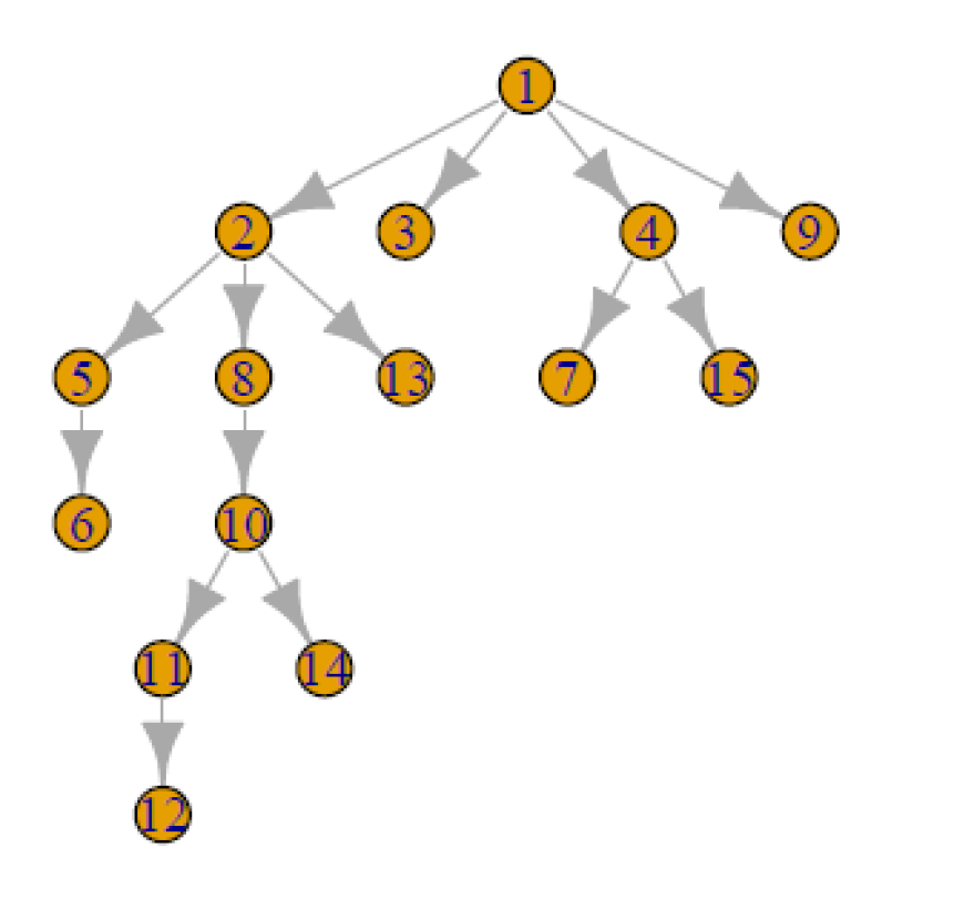
Consider a 15-node Bayesian network (BN), an example of which is visualized in Figure 1. One common field in BN analysis is structure discovery, in which the goal is to identify relationships among a set of variables which are each visualized by a node. In the example given in Figure 1, we see that node 1 (representing variable 1) has a direct relationship with node 2, but an indirect relationship with node 13, as there is no arrow drawn directly from 1 to 13. We represent these relationships with the parameters , in which if there is an arrow drawn from node to node , and otherwise. Note that in a 15-node BN space there are 210 such parameters.
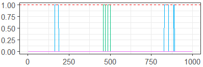
To provide an example, we simulated data from a 15-node Bayesian network and used the partition-MCMC algorithm [15] to sample 1000 iterations of 5 chains, each from a posterior distribution defined on the space , the space of 15-node Bayesian networks. Figure 2 gives a univariate traceplot of the arrow-existence parameter
Because the parameter in question is binary, the information gained by viewing the traceplot is very limited. The situation is clearly very unlikely, but does the fact that the sampler doesn’t often include it in the model actually demonstrate that the sampler is not performing well?
Additionally, univariate measures of the effective sample size or potential scale reduction factor are equally useless as both assume there will be some level of variability per parameter. Multivariate versions of these diagnostics may fare better, but will still struggle as they assume a Euclidean paradigm in this high-dimensional non-Euclidean space.
A decent solution to this problem is to produce traceplots (and potentially calculate univariate diagnostics) using the posterior value or likelihood evaluated at each MCMC sample [11, 13]. However, this approach is flawed when the parameter space includes multiple modes of similar likelihood, as is common (and unpredictable) in many modern high-dimensional applications. In these situations, any likelihood-based diagnostics fail to identify the difference between the modes.
In Section 4.2 below, we present a generalized traceplot on the same MCMC samples which incorporates information from all variables, and clearly demonstrates that the sampler is failing to mix adequately.
2.2 Non-Euclidean MCMC Movement
To explore potential consequences of non-Euclidean MCMC moves, we consider a hypothetical scenario in which a statistician (we’ll call him Luke) wants to sample from a univariate distribution on the random variable using an MCMC algorithm. The distribution is an equal parts mixture of three normal distributions , where and Due to the small standard deviations, the three parts of the mixture essentially don’t overlap at all. We denote this sampling space and distribution using , as it is tri-modal.
In an effort to ensure good results, Luke uses two different MCMC samplers to draw from . is a typical Metropolis-Hastings algorithm in which proposed draws follow the distribution , where is the current draw. However, attempting to cleverly improve the rate at which mixing is achieved, Luke builds as a Metropolis-Hastings algorithm with a proposal distribution that is an equal parts mixture of a normal distribution centered at the current draw with standard deviation .1, and a normal distribution centered at the negative of the current draw with standard deviation .1. That is, proposed draws follow the distribution
where
The thought behind is that a lower standard deviation will improve the mixing within each mode, and that taking approximately half of the draws from a distribution centered at instead of will allow for the algorithm to effectively move between the two outside modes (Luke apparently forgot about the mode centered at 0).
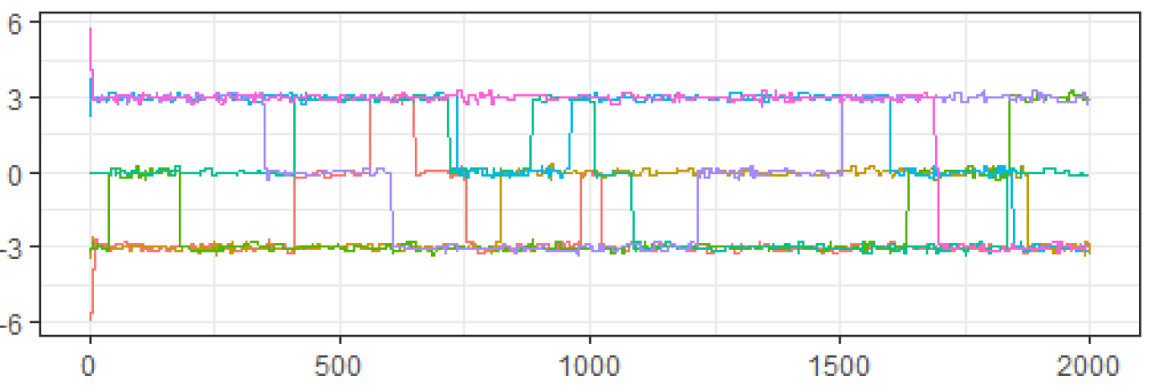
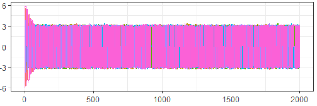
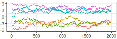
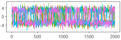
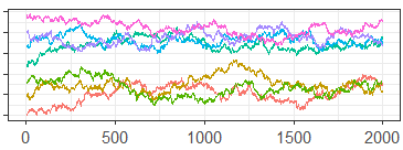
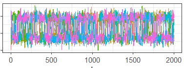
Both samplers were then run on 7 chains of 2000 draws each, starting at the points Figures 3 and 4 show the traceplots of the draws from Samplers 1 and 2 respectively, while Table 1 presents the ESS and PSRF.
| Standard ESS | Standard PSRF | |
|---|---|---|
| 46.27 | 1.42 | |
| 6237.28 | 1.01 |
Looking at the diagnostics for , we see that because the traceplot is clearly not mixing well across modes, the ESS is very low, and the PSRF is much larger than the recommended 1.01, we should not use the results from . In contrast, for the traceplot looks like it is mixing well, the ESS is high, and the PSRF is 1.01. Thus, based on these diagnostics, it appears that we should accept the results from .
However, as could be guessed by the strange construction of the proposal distribution, is also failing to mix well and results in a very bad approximation of the target distribution. In fact, if we define to be the target distribution, and to be the empirical distributions given by the draws from Samplers 1 and 2 respectively, and to be the Kullback-Leibler divergence, then while . That is, the divergence between and is 7-times worse than the divergence between and . This is mainly due to the fact that, while 1/3 of is concentrated in the central mode, only 1/7 of the draws making up are from the central mode.
Clearly, was a bad idea from the beginning as it avoided the mode centered at 0 almost entirely. However, the traceplot, ESS and PSRF all appeared to show good mixing for . If an ill-considered MCMC algorithm was able to fool our selected set of diagnostics so completely, we need to understand why. After all, most practical applications of MCMC algorithms do not operate in clearly-defined univariate spaces where poorly-constructed algorithms are easily spotted from the start.
The problem here lies in the distinction between the distance being used by the algorithm vs. the distance being used by the diagnostic. Traceplots, the univariate effective sample size, and the univariate potential scale reduction-factor all assume that distances between draws in an MCMC algorithm are Euclidean. This assumption works in the case of as, defining the current draw as , moving to a different value becomes monotonically less likely as the Euclidean distance between and increases.
However, operates with a different understanding of distance. Given that the current draw is , the probability of moving to no longer monotonically decreases as the Euclidean distance increases. In fact, if , we know for most of our sample space that the probability of moving from to is greater than the probability of moving from to 0, despite the fact that This is represented using a heatmap in Figure 5, which shows (among other things) that the probability of moving from -3 to 3, is much higher than the probability of moving from -3 to 0.
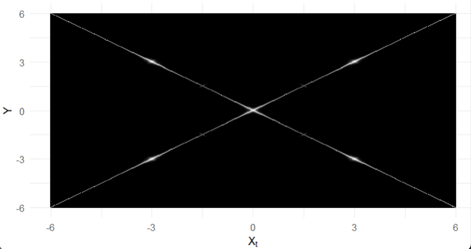
This discrepancy in definitions of distance causes all of the problems in the convergence diagnostics shown for . For the traceplot, the fact that most of the chains regularly bounce between modes at -3 and 3 obscures the fact that most chains never visit the mode at 0. Here the traceplot’s notion of Euclidean distance (which assumes that 0 falls between -3 and 3) is in conflict with the distance used by which essentially treats -3 and 3 as identical points, with nothing in between them.
Then, notice that both ESS and the PSRF are based on the sum of squared errors around chain means. Since the sample mean is a measure of central tendency with respect to the Euclidean distance, if a chain bounces back and forth between the modes at -3 and 3, the chain mean will be somewhere around 0. However, the chain never visits anywhere near 0, and so the sample mean fails as a true measure of central tendency in terms of the MCMC movements of .
In Section 4.3, we present generalized diagnostics that clearly demonstrate the lack of mixing in .
3 Generalized Convergence Diagnostics
In this section, we outline a method for creating generalized convergence diagnostics for any MCMC algorithm that accomplishes important goals related to the two case-studies presented above.
First, by allowing for flexibility in the notion of distance, we extend the work of [16] and provide easy access to standard convergence diagnostics in problems with a large number of binary or discrete parameters. Second, for MCMC algorithms based on non-Euclidean distances, we provide investigators with the means to evaluate the performance of MCMC samplers using non-standard moves.
In addition to solving the problems mentioned above, we seek to develop a solution that is generally applicable and easy to implement. Even when targeted convergence diagnostics are designed for application-specific MCMC samplers, they can be complex and difficult to implement. By providing the general algorithm below, along with guidance for use in multiple situations and an open-source package in R [7], we hope to make MCMC diagnostics more accessible to investigators, regardless of the sampling context. We begin our discussion of the algorithm by defining our use of two key terms.
Definition 1.
Let be a parameter space, let and let be an MCMC algorithm defined on .
A distance is a function defined on the cross-product of with itself such that for all . Our goal with a distance is to establish a relevant notion of ‘nearness’ on the parameter space and as such we will use terminology such as ‘far apart’ when is large, and ‘close together’ when it is small. Please note that we do not require to be a metric in the formal mathematical sense.
A proximity-map is a function that depends on the distance and which maps the parameter space to the real line in such a way as to place values close together(far apart) in that are close together (far apart) in . This definition is obviously very loose and does not allow for rigorous analysis. However, this is necessary to allow for a variety of functional proximity-maps as a natural trade-off exists between a proximity-map’s faithfulness to the defined distance, and the computational time required to use it.
We now present the psuedo-code for the Generalized Convergence Diagnostic algorithm which takes typically multivariate chains, each of length , transforms them into univariate chains using , and evaluates the desired convergence diagnostic on the univariate chains.
This is, of course, a very high-level view of generalized diagnostics that obscures much of the nuance determining whether or not the diagnostics will be informative. However, the general idea is clear. Generalized convergence diagnostics are created by choosing a relevant distance, choosing a proximity-map based on that distance, and then mapping all draws from the sampler to the real line. Once the values are mapped, standard convergence diagnostics are evaluated on the newly univariate MCMC chains.
Note that, as with other diagnostics, generalized convergence diagnostics presented in this paper (especially those related to effective sample size) should be interpreted approximately and used comparatively between different samplers. Additionally, consistent with other convergence literature, generalized convergence diagnostics cannot prove that a sampler is mixing well, they can only demonstrate a lack of mixing. However, as we will demonstrate in the simulation studies, when used properly, generalized convergence diagnostics can be incredibly helpful in diagnosing issues with sampler mixing and convergence.
3.1 Choosing a Distance
Selecting a distance function on to use with a sampler involves evaluating and prioritizing several important factors. First, in order to be relevant, must at least somewhat reflect the movement of in the sample space . That is, if with , then if is currently at , should generally be a more-likely next move than . This is the most obvious requirement for , and is fulfilled quite clearly by standard convergence diagnostics based on the Euclidean distance. If this requirement is not met (at least for the majority of sampling steps) the diagnostic measures will register frequent movements by the sampler that appear to be very large, but are in reality, much smaller (this was the fundamental problem in our second case-study). This requirement of relevance to can be difficult to accomplish, particularly when a sampler has different ‘types’ of moves that it can choose from, like a split-merge step in a DPMM. However, we have found distance functions to be successful in identifying mixing issues as long as agrees with in the large majority of draws.
Second, the distance function should be relevant to the diagnostic target. If is a ten dimensional parameter space and is defined to ignore nine of those dimensions, the resulting diagnostics will only be applicable to the mixing of the one parameter included in the definition. Defining to ignore particular dimensions of the parameter space can be useful as it can allow for examination of sampler mixing on groups of related or important parameters, but should be done with caution knowing that information is being excluded.
Third, computational time should be considered when defining . Depending on the proximity-map (which we will discuss in Section 3.2), may need to be evaluated as many as times (or as few as times), where is the total number of unique draws across all chains. If is slow to calculate and is large, this can lead to exceedingly long computation times, rendering the diagnostic process largely useless. With these considerations in mind we provide two examples of distance functions that we have found useful in application.
3.1.1 The Hamming Distance
Let be the set of all matrices with binary entries. Let . The Hamming distance between and , defined as is simply the number of entries in that differ from . The Hamming distance is very flexible and may be applied in many MCMC applications of interest.
For example, tree structures may be represented with matrices in which a value of 1 in the th position indicates the existence of an edge between the and nodes. As discussed in the Introduction, the Hamming distance defined on tree structures is used by Lanfear et al. to develop generalized traceplots and calculate a generalized effective sample size[16].
As another example, a sample from a Dirichlet Process Mixture Model provides a clustering of observations. An matrix , called the co-association matrix, may be defined such that if observations and are assigned to the same cluster [10]. Generalized convergence diagnostics may be evaluated using the Hamming distance defined on these co-association matrices.
The Hamming distance offers the advantages of (relatively) quick computation and very clear interpretability. Additionally, the Hamming distance is frequently related to the most important aspects of the inference question at hand (structure for trees, clusterings for DPMMs).
3.1.2 The Metropolis-Hastings Distance
The Metropolis-Hastings (MH) algorithm is a particular form of an MCMC algorithm that is popular in many fields of Bayesian inference due to its highly flexible formulation [3]. The core of the algorithm relies on two different density functions, the target density and a conditional density , called the ‘proposal density’. In the following, we assume that the conditional density is symmetric in the sense that for all The derivations for the non-symmetric case are similar.
The MH algorithm for picking the next point from current point operates as follows:
-
1.
Sample a proposed point from the proposal density
-
2.
Calculate an acceptance probability
-
3.
Generate a uniform random number .
-
4.
If , set , otherwise set
Because of the widespread use of this algorithm, we propose the complementary Metropolis-Hastings distance as a distance function that allows convergence diagnostics to accurately reflect the movement of a MH algorithm. The Metropolis-Hastings is defined as:
where We will work from the inside out in our exploration of this definition.
First, observe that, if the current point is then we must have where the value approaches 1 when is more likely to be sampled, and approaches 0 when is less likely to be sampled. Thus, the quantity can be seen as the acceptance probability multiplied by a value that reflects the probability of being proposed given . Therefore, can be interpreted as a pseudo-probability of moving to point given that the current point is point . An identical interpretation of may be used if the current point is and the proposed point is .
The minimum around these two terms is used to ensure that While many binary operators could be used to guarantee this property we selected the minimum as it best reflects an equal combination of the posterior and proposal densities. We also considered the mean or maximum, but both were influenced much more by changes in the proposal density and were less affected by changes in the posterior.
Finally, we subtract the minimum term from one so that implies that the algorithm views and as essentially the same point, and implies that the probability the algorithm will move from to (or vice versa) is 0.
The Metropolis-Hastings distance has several nice properties. First, it is highly versatile and may be used as a distance for any MH MCMC algorithm. Additionally, it is directly related to the notion of distance used by a corresponding MH algorithm and ensures that implies that the algorithm is more likely to move to than to if the current point is Finally, it incorporates all of the information used by the MCMC algorithm and therefore encompasses all information of interest in the inference.
The most significant issue with the MH distance is computation time. For more complex MH algorithms with multiple steps, evaluating the posterior or proposal may be relatively slow, and doing so times will become computationally prohibitive. However, if computational time is not an issue, or the MH sampler is simple, using can result in very insightful convergence diagnostics. See Section 4.3 for an example of diagnostics based on , which reveal the problems explored in the case-study in Section 2.2.
3.2 Choosing a Proximity-Map
The proximity-map must, at least in part, be based on the selected distance function. Remaining fully faithful to a particular definition of distance is difficult when performing any sort of dimension reduction or mapping, especially in higher dimensions, but may also be difficult in lower dimensions. However, some effort must be made in order to ensure that the resulting diagnostics are informative. Standard dimensionality reduction techniques, such as random projections or principle component analysis, assume a Euclidean distance paradigm and would not serve as effective proximity-maps, unless your distance function is the Euclidean distance. As we will demonstrate in the examples below, the notion of ’remaining faithful’ to the distance function can be quite loose in application and still get excellent results.
The second consideration, also very important, is computation time. Generally speaking, proximity-maps that are more faithful to the distance function also tend to be more difficult to compute. Selecting a good proximity-map essentially comes down to a trade-off between the two. Diagnostic measures that take too long to compute are not particularly useful, but neither are diagnostic measures that fail to reveal mixing or convergence issues. We now present two examples of proximity-maps and discuss the costs and benefits associated with each.
3.2.1 The Lanfear Proximity-map
In the Introduction we discussed a method of traceplot creation and ESS calculation explored by Lanfear et al. in [16]. Here we generalize their method into our proposed framework and refer to the mapping created as the Lanfear proximity-map.
Formally, the Lanfear proximity-map based on distance with reference point , is the function . Plugging this in as the proximity-map for Algorithm 1, notice that this requires to be evaluated exactly times, where is the number of MCMC draws across all chains. This means that is quite computationally reasonable, and typically evaluates very quickly.
Unfortunately, algorithmic speed comes at the cost of dependence on a reference point . While this is not always an issue, it is not difficult to find examples, some of which we show in Section 4, in which the dependence on a reference point causes problems with the resulting convergence diagnostics.
3.2.2 The Nearest Neighbor Proximity-map
The Nearest Neighbor proximity-map, denoted by , is based on the Nearest Neighbor algorithm which is a greedy graph-theoretic algorithm that provides a solution to the well-known Traveling Salesman problem (TSP) [20].
Starting with a collection of unique points and a distance function , the Nearest Neighbor algorithm produces an ordering of by picking a random point and then, step by step, moving to the next closest node (in terms of the distance function ) that has not been previously selected, until ending back at the starting point. This is outlined in psuedo-code in Algorithm 2.
The Nearest Neighbor algorithm can be used to take a set of unique sampled values from and produce a cyclic ordering of those samples that respects a distance , which is a good foundation for a proximity-map. However, in defining , we require an additional step.
The output provided by Algorithm 2 is a cycle, ending where it began, and not a true ordering. As we plan to map sampled values to the real-line respecting our distance-based ordering, we need to identify a place to ‘cut’ our cycle (the cut-point) so that we have a beginning and ending in the mapped values. We describe our cut-point selection method here.
Let be the ordering of created by cutting the cycle provided by the NN algorithm between and , for . We will define a proximity-map based on for all and choose the map that minimizes a target distance defined below. Intuitively, we define to be the distance travelled if moving from to point-by-point along the sequence . Specifically, we recursively define by
for all , and As an example we have written out here:
Now, as defined above, let be the th chain of length drawn from . Define
While the definition of is quite involved, it is actually a rather intuitive construct. Consider drawing a traceplot of all chains after applying the proximity-map simply measures the vertical distance travelled by chain under this mapping. A (relatively) large value of can imply that the chain travels from near the top to near the bottom of the traceplot’s -axis frequently. If a single chain travels in this way it can obscure information about the other chains on the traceplot, as well as lower the accuracy of other univariate multi-chain diagnostics. Thus, we choose to be the proximity-map
The psuedo-code for generating the Nearest Neighbor proximity-map is described in Algorithm 3.
The Nearest Neighbor proximity-map has several advantages over the Lanfear proximity-map. First, because it is based on pairwise distances between all unique draws and not just a single reference point, it frequently captures more of the true sample space in the final mapping. Additionally, distance functions which have a maximum possible distance (such as ) can be uninformative when used with the Lanfear proximity-map as frequently 50% or more of the sampled values are at the maximum distance possible away from any given point and therefore all information about those far-away points are lost. This is not a problem with since it is a global rather than a local map.
However, the Nearest Neighbor proximity-map is significantly more computationally-intensive, particularly when the number of unique drawn values is very large. Additionally, as is well-documented, the Nearest Neighbor algorithm is sensitive to the choice of the starting point. This doesn’t affect the Nearest Neighbor proximity-map as badly as the Lanfear proximity-map, but it is an important issue to be aware of.
4 Examples
Here we provide several simulated examples demonstrating the capabilities of generalized convergence diagnostics.
4.1 Bi-Modal Distribution
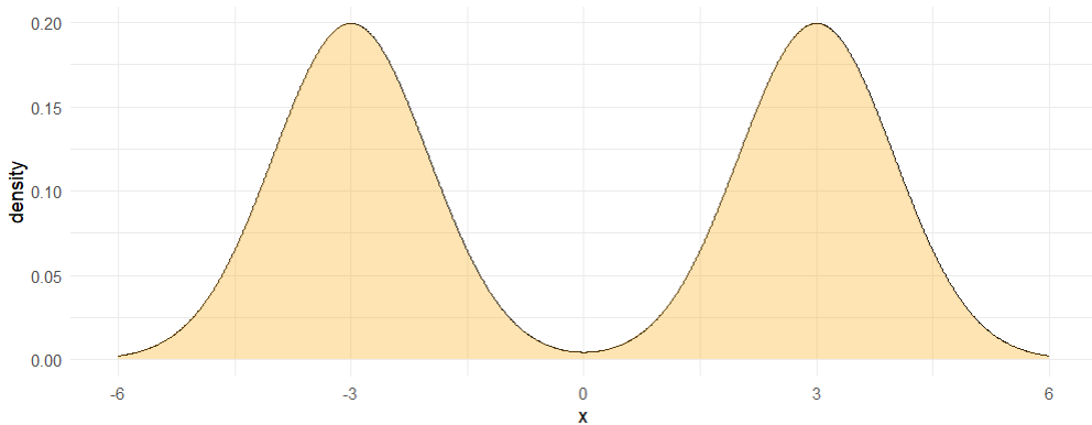
We begin with a simple bi-modal distribution on the real line, and denote this sample space . is constructed as an equal-parts mixture of two normal distributions, one centered at -3 and the other at 3, both with standard deviation 1. The posterior is visualized in Figure 6.
For this simulation we use two different MCMC samplers, denoted and , both defined on . Both and are Metropolis-Hastings algorithms with normal proposal distributions, centered at the current draw. The only difference is that the proposal distribution for has standard deviation .1, and so will have difficulty crossing between the two modes, while the proposal for has standard deviation 2. For each algorithm we draw 7 chains beginning at points (-6, -4, -2, 0, 2, 4, 6) and run each chain for 2000 iterations.
| Sampler | Standard ESS | Standard PSRF |
|---|---|---|
| 127.35 | 4.87 | |
| 393.12 | 1.02 |
Figure 7 shows the standard traceplots for algorithms and , while Table 2 gives the ESS and PSRF, calculated in the typical way. Based on the separation of chains and high auto-correlation in the traceplot, as well as the low ESS and PSRF much higher than the recommended 1.01, does not appear to be mixing well at all. In contrast, the (somewhat) well-mixed traceplot for , along with a higher ESS and much lower PSRF, suggest draws that are much closer to convergence.
Now consider the generalized diagnostics given in Figure 8 and Table 3. These are the traceplot, ESS and PSRF derived from using the Generalized Convergence Diagnostic algorithm with the Euclidean distance and Nearest Neighbor proximity-map. As we would hope, since standard diagnostics are also based on the Euclidean distance, these diagnostics are almost identical to the standard diagnostics. This demonstrates that our generalized diagnostics can be viewed as approximate extensions of standard diagnostics.
| Generalized ESS | Generalized PSRF | |
|---|---|---|
| 127.36 | 4.87 | |
| 386.76 | 1.02 |
4.2 Bayesian Network
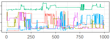
In Section 2.1 we presented a short example of a standard traceplot on a binary parameter from a 15-node Bayesian network. As discussed in Section 2.1, the standard traceplot was almost entirely useless, and was not informative about the mixing of the MCMC algorithm. While there are other methods of diagnosing convergence in such models, in order to demonstrate the capabilities of our approach, we show a generalized traceplot of the same MCMC samples based on the Hamming distance and Nearest Neighbor proximity-map in Figure 9. Using this traceplot it is immediately apparent that our sampler is mixing very poorly. This can be seen by the significant number of flat lines suggesting failures of the MCMC sampler to move from a single point, and by the chain represented by the green line which appears to be sampling from an entirely different portion of the sample space as the rest of the chains.
4.3 Tri-Modal Distribution
In Section 2.2 we introduced a tri-modal distribution on the real line . Draws using the simple algorithm were clearly not mixing, while draws from a more complex, but worse algorithm appeared to be mixing based on standard convergence diagnostics. Here we present Figure 10, a generalized traceplot for the draws from created using the Metropolis-Hastings distance and the Nearest Neighbor proximity-map, and Table 4 which gives the generalized ESS and PSRF calculated using the same method. Note that both the traceplot and the PSRF clearly reveal a lack of between-chain convergence, while the ESS is much lower (and certainly more accurate) than the ESS calculated using the Euclidean distance in Section 2.2.
| Generalized ESS | Generalized PSRF | |
|---|---|---|
| 984.76 | 2.84 |
4.4 Dirichlet Process Mixture Model
The Dirichlet Process Mixture Model (DPMM) may be used to cluster observations into latent groups, and is unique in that its construction does not require that the number of groups be specified a priori. The algorithm and its theoretical justification were introduced approximately 50 years ago [2, 8, 9].
A unique problem when using an MCMC sampler to perform inference with a DPMM is that the number of parameters at each iteration may change as latent mixture components are added or deleted. For example, at the start of a given MCMC iteration to fit a DPMM using a mixture of Gaussians, there may be three latent components. Since each component has its own group-specific mean and variance parameters, we start the iteration with three mean vectors , and three covariance matrices . However, as we iterate through the observed values assigned to each of the three components, the MCMC sampler may assign one or more observations to a previously nonexistent fourth group. Thus, at the start of the next iteration our parameter space will consist of and .
In terms of MCMC diagnostics, there are two issues here: (1) the multivariate nature of the data, and (2) the expansion (and contraction) of the number of latent components, and thus the dimension of the parameter space over the course of the MCMC as described above. This second issue in particular is not handled well by current diagnostic tools. In order to make traceplots or calculate the values of MCMC diagnostics, one must condition on the number of latent components found at each MCMC iteration, and evaluate diagnostics on those results separately. These MCMC iterations are not necessarily contiguous after conditioning, so this process results in an incomplete or potentially misleading picture of the path of the MCMC. A common solution is to simply plot the log-likelihood at each iteration. However, as discussed in Section 2.1, this practice can obscure information when the posterior space is multi-modal.
| Generalized ESS | Generalized PSRF | |
|---|---|---|
| 1000.146 | 1.01 |
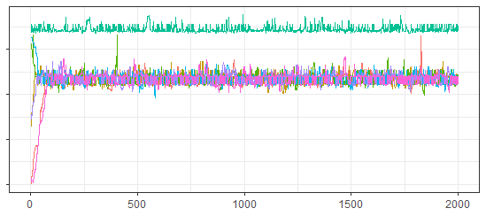
To demonstrate the utility of the generalized diagnostics introduced in this paper, we simulated data from a mixture of three Gaussian densities, denoted , and used it to fit a DPMM. The true component means are , , and , variances are all , and the mixing proportions are . We fit a DPMM with a diagonal covariance structure, setting a normal prior on the mean parameters and an inverse gamma prior on the diagonal variance . Using Algorithm 2 from Neal [19], we learned parameters , and for latent groups (noting again that changes between iterations). We ran five chains with this MCMC sampler, denoted , for 12,000 iterations each including 2,000 burn-in iterations. Each chain was initialized at a different place, with either 1,2,3,4 or 5 latent components.
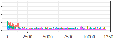
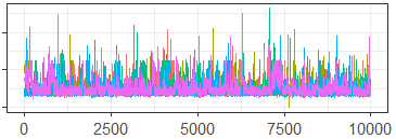
The generalized diagnostic tables and plots for sampling from this space are provided in Figures 11-12, and Table 5. These generalized diagnostics use the Hamming distance on the co-association matrices from each MCMC iteration, and the Lanfear proximity-map. Figure 11 shows major differences between the chains during the burn-in period, the scale of which distorts the remaining iterations. In Figure 12, we include only the iterations from after the burn-in, and note that the sampler appears to demonstrate some signs of lack of convergence between chains, although overall the chains appear to be moving in similar spaces. While the generalized ESS and PSRF look good, the DPMM in this instance does warrant some additional investigation to ensure that the occasional points when the MCMC chains appear trapped in different modes are not interfering with the overall inference.
5 Discussion
The method of deriving generalized convergence diagnostics presented in this paper is highly flexible and capable of solving several issues facing MCMC convergence diagnostics simultaneously. First, by focusing on reducing each MCMC iteration down to a single dimension through the distance and proximity-map functions, our method provides quick and interpretable visualizations and diagnostics on high-dimensional MCMC problems. Second, by allowing for non-Euclidean understandings of the distance between MCMC iterations, our method is able to identify issues that elude other commonly used diagnostic measures, and to our knowledge, is the first method to address non-Euclidean MCMC moves in a generalized way. Finally, by keeping the method generalized and including the publicly available R package genMCMCDiag, we present a method that is both widely-applicable and easy to access. While we do not anticipate that our generalized diagnostics are able to outperform diagnostics that are custom-tailored to a research problem, applying our method will provide good insight into convergence issues while costing many fewer research-hours.
Future research areas are primarily focused on the distance and proximity-map functions. As these functions are integral to the success of the diagnostics we hope to identify more distance and proximity-map options, and improved guidelines for choosing options for a specific case. Future investigation on options for distance functions will seek to both broaden the applicability of our method, as well as provide an approach for honing in on particular issues in specific models and situations. Continuing research for choices of proximity-maps will target both improved responsiveness to the distance function, and faster computational times.
Declaration of Competing Interest:
There is no competing interest.
Acknowledgements:
The authors would like to thank Serge Aleshin-Guendel for his helpful suggestions of additional citations and applications for our work, and Luke Rosamilia for the title suggestion.
Research reported in this publication was supported by the National Institute of Environmental Health Sciences of the National Institutes of Health (NIH) under award numbers T32ES007271, T32ES007142, P30ES000002, and P42030990. The content is solely the responsibility of the authors and does not necessarily represent the official views of the NIH.
References
- [1] Serge Aleshin-Guendel and Rebecca C Steorts “Convergence Diagnostics for Entity Resolution” In Annual Review of Statistics and Its Application 11.1 Annual Reviews, 2024, pp. 419–435
- [2] Charles E Antoniak “Mixtures of Dirichlet processes with applications to Bayesian nonparametric problems” In The annals of statistics JSTOR, 1974, pp. 1152–1174
- [3] Siddhartha Chib and Edward Greenberg “Understanding the Metropolis-Hastings algorithm” In The American Statistician 49.4 Taylor & Francis, 1995, pp. 327–335
- [4] Mary Kathryn Cowles and Bradley P Carlin “Markov chain Monte Carlo convergence diagnostics: a comparative review” In Journal of the American Statistical Association 91.434 Taylor & Francis, 1996, pp. 883–904
- [5] Benjamin E Deonovic and Brian J Smith “Convergence diagnostics for MCMC draws of a categorical variable” In arXiv preprint arXiv:1706.04919, 2017
- [6] Anand Dixit and Vivekananda Roy “MCMC diagnostics for higher dimensions using Kullback Leibler divergence” In Journal of Statistical Computation and Simulation 87.13 Taylor & Francis, 2017, pp. 2622–2638
- [7] Luke Duttweiler “genMCMCDiag: Generalized Convergence Diagnostics for Difficult MCMC Algorithms” R package version 0.2.1, 2024 URL: https://CRAN.R-project.org/package=genMCMCDiag
- [8] Thomas S Ferguson “A Bayesian analysis of some nonparametric problems” In The annals of statistics JSTOR, 1973, pp. 209–230
- [9] Thomas S Ferguson “Bayesian density estimation by mixtures of normal distributions” In Recent advances in statistics Elsevier, 1983, pp. 287–302
- [10] Ana LN Fred and Anil K Jain “Combining multiple clusterings using evidence accumulation” In IEEE transactions on pattern analysis and machine intelligence 27.6 IEEE, 2005, pp. 835–850
- [11] Nir Friedman and Daphne Koller “Being Bayesian about network structure. A Bayesian approach to structure discovery in Bayesian networks” In Machine learning 50.1 Springer, 2003, pp. 95–125
- [12] Andrew Gelman and Donald B Rubin “Inference from iterative simulation using multiple sequences” In Statistical science 7.4 Institute of Mathematical Statistics, 1992, pp. 457–472
- [13] Marco Grzegorczyk and Dirk Husmeier “Improving the structure MCMC sampler for Bayesian networks by introducing a new edge reversal move” In Machine Learning 71.2-3 Springer, 2008, pp. 265
- [14] Sonia Jain and Radford M Neal “A split-merge Markov chain Monte Carlo procedure for the Dirichlet process mixture model” In Journal of computational and Graphical Statistics 13.1 Taylor & Francis, 2004, pp. 158–182
- [15] Jack Kuipers and Giusi Moffa “Partition MCMC for inference on acyclic digraphs” In Journal of the American Statistical Association 112.517 Taylor & Francis, 2017, pp. 282–299
- [16] Robert Lanfear, Xia Hua and Dan L Warren “Estimating the effective sample size of tree topologies from Bayesian phylogenetic analyses” In Genome biology and evolution 8.8 Oxford University Press, 2016, pp. 2319–2332
- [17] Andrew Magee, Michael Karcher, Frederick A Matsen IV and Volodymyr M Minin “How trustworthy is your tree? Bayesian phylogenetic effective sample size through the lens of Monte Carlo error” In Bayesian Analysis 19.2 International Society for Bayesian Analysis, 2024, pp. 565–593
- [18] Théo Moins, Julyan Arbel, Anne Dutfoy and Stéphane Girard “On the use of a local ˆR to improve MCMC convergence diagnostic” In Bayesian Analysis 1.1 International Society for Bayesian Analysis, 2023, pp. 1–26
- [19] Radford M Neal “Markov chain sampling methods for Dirichlet process mixture models” In Journal of computational and graphical statistics 9.2 Taylor & Francis, 2000, pp. 249–265
- [20] Gerhard Reinelt “The traveling salesman: computational solutions for TSP applications” Springer, 2003
- [21] Vivekananda Roy “Convergence diagnostics for Markov chain Monte Carlo” In Annual Review of Statistics and Its Application 7 Annual Reviews, 2020, pp. 387–412
- [22] Chengwei Su and Mark E Borsuk “Improving structure mcmc for Bayesian networks through Markov blanket resampling” In The Journal of Machine Learning Research 17.1 JMLR. org, 2016, pp. 4042–4061
- [23] Chris Whidden and Frederick A Matsen IV “Quantifying MCMC exploration of phylogenetic tree space” In Systematic biology 64.3 Oxford University Press, 2015, pp. 472–491