The two-edge connectivity survivable-network design problem in planar graphs

Glencora Borradaile
Oregon State University Philip Klein
Brown University

Abstract

Consider the following problem: given a graph with edge costs and a subset $Q$ of vertices, find a minimum-cost subgraph in which there are two edge-disjoint paths connecting every pair of vertices in $Q$ . The problem is a failure-resilient analog of the Steiner tree problem arising, for example, in telecommunications applications. We study a more general mixed-connectivity formulation, also employed in telecommunications optimization. Given a number (or requirement) $r(v)\in\{0,1,2\}$ for each vertex $v$ in the graph, find a minimum-cost subgraph in which there are $\min\{r(u),r(v)\}$ edge-disjoint $u$ -to- $v$ paths for every pair $u,v$ of vertices.

We address the problem in planar graphs, considering a popular relaxation in which the solution is allowed to use multiple copies of the input-graph edges (paying separately for each copy). The problem is max SNP-hard in general graphs and strongly NP-hard in planar graphs. We give the first polynomial-time approximation scheme in planar graphs. The running time is $O(n\log n)$ .

Under the additional restriction that the requirements are only non-zero for vertices on the boundary of a single face of a planar graph, we give a polynomial-time algorithm to find the optimal solution.

1 Introduction

In the field of telecommunications network design, an important requirement of networks is resilience to link failures [24]. The goal of the survivable network problem is to find a graph that provides multiple routes between pairs of terminals. In this work we address a problem concerning edge-disjoint paths. For a set $S$ of non-negative integers, an instance of the $S$ -edge connectivity design problem is a pair $(G,\bm{r})$ where $G=(V,E)$ is a undirected graph with edge costs $\bm{c}\;:\;V\rightarrow\Re^{+}$ and connectivity requirements $\bm{r}\;:\;V\rightarrow S$ . The goal is to find a minimum-cost subgraph of $G$ that, for each pair $u,v$ of vertices, contains at least $\min\{\bm{r}(u),\bm{r}(v)\}$ edge-disjoint $u$ -to- $v$ paths.

In telecommunication-network design, failures are rare; for this reason, there has been much research on low-connectivity network design problems, in which the maximum connectivity requirement is two. Resende and Pardalos [24] survey the literature, which includes heuristics, structural results, polyhedral results, computational results using cutting planes, and approximation algorithms. This work focuses on $\{0,1,2\}$ -edge connectivity problems in planar graphs.

We consider the previously studied variant wherein the solution subgraph is allowed to contain multiple copies of each edge of the input graph (a multi-subgraph); the costs of the edges in the solution are counted according to multiplicity. For $\{0,1,2\}$ -connectivity, at most two copies of an edge are needed. We call this the relaxed version of the problem and use the term strict to refer to the version of the problem in which multiple copies of edges of the input graph are disallowed.

A polynomial-time approximation scheme (PTAS) for an optimization problem is an algorithm that, given a fixed constant $\epsilon>0$ , runs in polynomial time and returns a solution within $1+\epsilon$ of optimal. The algorithm’s running time need not be polynomial in $\epsilon$ . The PTAS is efficient if the running time is bounded by a polynomial whose degree is independent of $\epsilon$ . In this paper, we focus on designing a PTAS for $\{0,1,2\}$ -edge connectivity.

Two edge-connected spanning subgraphs

A special case that has received much attention is the problem of finding a minimum-cost subgraph of $G$ in which every pair of vertices is two edge-connected. Formally this is the strict $\{2\}$ -edge connectivity design problem. This problem is NP-hard [12] (even in planar graphs, by a reduction from Hamiltonian cycle) and max-SNP hard [10] in general graphs. In general graphs, Frederickson and JáJá [13] gave an approximation ratio of 3 which was later improved to 2 (and 1.5 for unit-cost graphs) by Khuller and Vishkin [17]. In planar graphs, Berger et al. [4] gave a polynomial-time approximation scheme (PTAS) for the relaxed $\{1,2\}$ -edge connectivity design problem and Berger and Grigni [5] gave a PTAS for the strict $\{2\}$ -edge connectivity design problem. Neither of these algorithms is efficient; the degree of the polynomial bounding the running time grows with $1/\epsilon$ . For the relaxed version of spanning planar 2-edge connectivity, the techniques of Klein [19] can be used to obtain a linear-time approximation scheme.

Beyond spanning

When a vertex can be assigned a requirement of zero, edge-connectivity design problems include the Steiner tree problem: given a graph with edge costs and given a subset of vertices (called the terminals), find a minimum-cost connected subgraph that includes all vertices in the subset. More generally, we refer to any vertex with a non-zero connectivity requirement as a terminal. For $\{0,2\}$ -edge connectivity design problem, in general graphs, Ravi [23] showed that Frederickson and JáJá’s approach could be generalized to give a 3-approximation algorithm (in general graphs). Klein and Ravi [20] gave a 2-approximation for the $\{0,1,2\}$ -edge connectivity design problem. (In fact, they solve the even more general version in which requirements $\bm{r}({u,v})$ are specified for pairs $u,v$ of vertices.) This result was generalized to connectivity requirements higher than two by Williamson et al. [27], Goemans et al. [14], and Jain [16]. These algorithms each handle the strict version of the problem.

In their recent paper on the spanning case [5], Berger and Grigni raise the question of whether there is a PTAS for the $\{0,2\}$ -edge connectivity design problem in planar graphs. In this paper, we answer that question in the affirmative for the relaxed version. The question in the case of the strict version is still open.

1.1 Summary of new results

Our main result is a PTAS for the relaxed $\{0,1,2\}$ -edge connectivity problem in planar graphs:

Theorem 1.1.

For any $\epsilon$ , there is an $O(n\log n)$ algorithm that, given a planar instance $(G,\bm{r})$ of relaxed $\{0,1,2\}$ -edge connectivity, finds a solution whose cost is at most $1+\epsilon$ times optimal.

This result builds on the work of Borradaile, Klein and Mathieu [7, 8, 9] which gives a PTAS for the Steiner tree (i.e. $\{0,1\}$ -edge connectivity) problem. This is the first PTAS for a non-spanning two-edge connectivity problem in planar graphs.

Additionally, we give an exact, polynomial-time algorithm for the special case where are the vertices with non-zero requirement are on the boundary of a common face:

Theorem 1.2.

There is an $O(k^{3}n)$ -time algorithm that finds an optimal solution to any planar instance $(G,\bm{r})$ of relaxed $\{0,1,2\}$ -edge-connectivity in which only $k$ vertices are assigned nonzero requirements and all of them are on the boundary of a single face. For instances of relaxed $\{0,2\}$ -edge connectivity (i.e. all requirements are 0 or 2), the algorithm runs in linear time.

1.2 Organization

We start by proving Theorem 1.2 in Section 3. The proof of this result is less involved and provides a good warm-up for the proof of Theorem 1.1. The algorithm uses the linear-time shortest-path algorithm for planar graphs [15] and a polynomial-time algorithm for the equivalent boundary Steiner-tree problem [11] as black boxes.

In order to prove Theorem 1.1, we need to review the framework developed for the Steiner tree problem in planar graphs. We give an overview of this framework in Section 4 and show how to use it to solve the relaxed $\{0,1,2\}$ -edge connectivity problem. The correctness of the PTAS relies on a Structure Theorem (Theorem 4.6) which bounds the number of interactions of a solution between different regions of the graph while paying only a small relative penalty in cost. We prove this Structure Theorem in Section 5. The algorithm itself requires a dynamic program; we give the details for this in Section 6.

2 Basics

We consider graphs and multi-subgraphs. A multi-subgraph is a subgraph where edges may be included with multiplicity. In proving the Structure Theorem we will replace subgraphs of a solution with other subgraphs. In doing so, two of the newly introduced subgraphs may share an edge.

For a subgraph $H$ of a graph $G$ , we use $V(H)$ to denote the set of vertices in $H$ . For a graph $G$ and set of edges $E$ , $G/E$ denotes the graph obtained by contracting the edges $E$ .

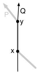
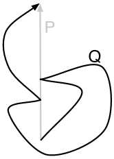
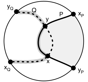
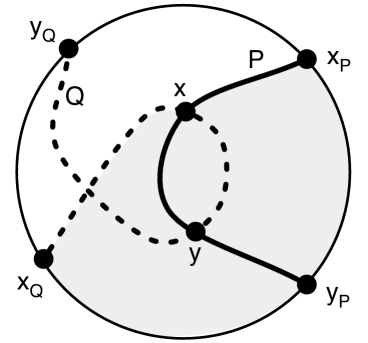
For a path $P$ , $P[x,y]$ denotes the $x$ -to- $y$ subpath of $P$ for vertices $x$ and $y$ of $P$ ; $\text{end}(P)$ and $\text{start}(P)$ denote the first and last vertices of $P$ ; $\text{rev}(P)$ denotes the reverse of path $P$ . For paths $A$ and $B$ , $A\circ B$ denotes the concatenation of $A$ and $B$ . See Figure 1 for an illustration of the notion of paths crossing. A cycle is non-self-crossing if every pair of subpaths of the cycle do not cross.

We employ the usual definitions of planar embedded graphs. For a face $f$ , the cycle of edges making up the boundary of $f$ is denoted $\partial f$ . We assume the planar graph $G$ is connected and is embedded in the plane, so there is a single infinite face, and we denote its boundary by $\partial G$ .

For a cycle $C$ in a planar embedded graph, $C[x,y]$ denotes an $x$ -to- $y$ path in $C$ for vertices $x$ and $y$ of $C$ . There are two such paths and the choice between the two possibilities will be disambiguated by always choosing the subpath in the clockwise direction. A cycle $C$ is said to enclose the faces that are embedded inside it. $C$ encloses an edge/vertex if the edge/vertex is embedded inside it or on it. In the former case, $C$ strictly encloses the edge/vertex. For non-crossing $x$ -to- $y$ paths $P$ and $Q$ , $P$ is said to be left of $Q$ if $P\circ\text{rev}(Q)$ is a clockwise cycle.

Refer to caption — Figure 1: (a) $P$ crosses $Q$ . (b) $P$ and $Q$ are noncrossing; $Q$ is left of $P$ (c) A self-crossing cycle. (d) A non-self-crossing cycle (non-self-crossing allows for repeated vertices, i.e. $v$ .)

We will use the following as a subroutine:

Theorem 2.1.

Erickson, Monma and Veinott [11] Let $G$ be a planar embedded graph with edge-costs and let $Q$ be a set of $k$ terminals that all lie on the boundary of a single face. Then there is an algorithm to find an minimum-cost Steiner tree of $G$ spanning $Q$ in time $O(nk^{3}+(n\log n)k^{2})$ or $O(nk^{3})$ time using the algorithm of [15].

2.1 Edge-connectivity basics

Since we are only interested in connectivity up to and including two-edge connectivity, we define the following: For a graph $H$ and vertices $x,y$ , let

c_{H}(x,y)=\min\{2,\text{maximum number of edge-disjoint $x$-to-$y$ paths in $H$}\}.

For two multi-subgraphs $H$ and $H^{\prime}$ of a common graph $G$ and for a subset $S$ of the vertices of $G$ , we say $H^{\prime}$ achieves the two-connectivity of $H$ for $S$ if $c_{H^{\prime}}(x,y)\geq c_{H}(x,y)$ for every $x,y\in S$ . We say $H^{\prime}$ achieves the boundary two-connectivity of $H$ if it achieves the two-connectivity of $H$ for $S=V(\partial G)$ .

Several of the results in the paper build on observations of the structural property of two-edge connected graphs. The first is a well-known property:

Lemma 2.2 (Transitivity).

For any graph $H$ , for vertices $u,v,w\in V(H)$ , $c_{H}(u,w)\geq\min\{c_{H}(u,v),c_{H}(v,w)\}$

Note that in the following, we can replace “strictly encloses no/strictly enclosed” with “strictly encloses all/strictly not enclosed” without loss of generality (by viewing a face enclosed by $C$ as the infinite face).

Lemma 2.3 (Empty Cycle).

Let $H$ be a (multi-)subgraph of $G$ and let $C$ be a non-self-crossing cycle of $H$ that strictly encloses no terminals. Let $H^{\prime}$ be the subgraph of $H$ obtained by removing the edges of $H$ that are strictly enclosed by $C$ . Then $H^{\prime}$ achieves the two-connectivity of $H$ .

Proof.

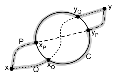
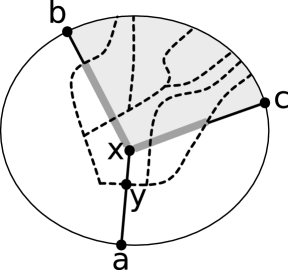
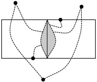
See Figure 2(b). Without loss of generality, view $C$ as a clockwise cycle. Consider two terminals $x$ and $y$ . We show that there are $c_{H}(x,y)$ edge-disjoint $x$ -to- $y$ paths in $H$ that do not use edges strictly enclosed by $C$ . There are two nontrivial cases:

$c_{H}(x,y)=1:$: Let $P$ be an $x$ -to- $y$ path in $H$ . If $P$ intersects $C$ , let $x_{P}$ be the first vertex of $P$ that is in $C$ and let $y_{P}$ be the last vertex of $P$ that is in $C$ . Let $P^{\prime}=P[x,x_{P}]\circ C[x_{P},y_{P}]\circ P[y_{P},y]$ . If $P$ does not intersect $C$ , let $P^{\prime}=P$ . $P^{\prime}$ is an $x$ -to- $y$ path in $H$ that has no edge strictly enclosed by $C$ .
$c_{H}(x,y)=2:$: Let $P$ and $Q$ be edge-disjoint $x$ -to- $y$ paths in $H$ . If $Q$ does not intersect $C$ , then $P^{\prime}$ and $Q$ are edge-disjoint paths, neither of which has an edge strictly enclosed by $C$ (where $P^{\prime}$ is as defined above). Suppose that both $P$ and $Q$ intersect $C$ . Define $x_{Q}$ and $y_{Q}$ as for $P$ . Suppose these vertices are ordered $x_{P}$ , $x_{Q}$ , $y_{Q}$ , $y_{P}$ around $C$ . Then $P[x,x_{P}]\circ C[x_{P},y_{Q}]\circ Q[y_{Q},y]$ and $Q[x,x_{Q}]\circ\text{rev}(C[y_{P},x_{Q}])\circ P[y_{P},y]$ are edge disjoint $x$ -to- $y$ paths that do not use any edges enclosed by $C$ . This case is illustrated in Figure 2; other cases (for other orderings of $\{x_{P},x_{Q},y_{Q},y_{P}\}$ along $C$ ) follow similarly.

We have shown that we can achieve the boundary two-connectivity of $H$ without using any edges strictly enclosed by a cycle of $H$ . The lemma follows. ∎

2.2 Vertex-connectivity basics

The observations in this section do not involve planarity. Although our results are for edge connectivity, we use vertex connectivity in Section 5 to simplify our proofs.

Vertices $x$ and $y$ are biconnected (a.k.a. two-vertex-connected) in a graph $H$ if $H$ contains two $x$ -to- $y$ paths that do not share any internal vertices, or, equivalently, if there is a simple cycle in $H$ that contains both $x$ and $y$ . For a subset $S$ of vertices of $H$ , we say $H$ is $S$ -biconnected if for every pair $x,y$ of vertices of $S$ , $H$ contains a simple cycle through $x$ and $y$ . We refer to the vertices of $S$ as terminals.

Lemma 2.4.

A minimal $S$ -biconnected graph is biconnected.

Proof.

Suppose $H$ has a cut-vertex $v$ : $H=H_{1}\cup H_{2}$ where $H_{1}\cap H_{2}=\{v\}$ and $H_{i}\neq\{v\}$ for $i=1,2$ . If $H_{1}$ and $H_{2}$ both have terminals then $H$ does not biconnect every pair of terminals. If, say, $H_{2}$ does not have a terminal then $H-(H_{2}-\{v\})$ is a smaller subgraph that biconnects the terminals. ∎

For the next two proofs, we use the notion of an (open) ear decomposition. An ear decomposition of a graph $G$ is a partition of the edges into a cycle $C$ and a sequence of paths $P_{1},P_{2},\ldots,P_{k}$ such that the endpoints of $P_{i}$ are in $C\cup(\bigcup_{j<i}P_{j})$ . The ear decomposition is open if the endpoints of $P_{i}$ are distinct. A graph is biconnected iff it has an open ear decomposition [25]. Ear decompositions can be built greedily starting with any cycle.

Theorem 2.5.

Let $H$ be a minimal $S$ -biconnected graph. Every cycle in $H$ contains a vertex of $S$ .

Proof.

Assume for a contradiction that $H$ contains a cycle $C$ that does not contain any terminals. By Lemma 2.4, $H$ is biconnected and so has an open ear decomposition starting with $C$ ; let $C,P_{1},P_{2},\ldots,P_{k}$ be an open ear decomposition of $H$ . Define $\mathcal{E}_{i}$ to be the subgraph composed of $C$ and the first $i$ ears: $C\cup(\bigcup_{j\leq i}P_{j})$ . We construct another open ear decomposition with one fewer ear $C^{\prime},P_{2}^{\prime},\ldots,P_{k}^{\prime}$ of $H$ as follows (note there is no ear $P_{1}^{\prime}$ ) and use $\mathcal{E}_{i}^{\prime}$ to denote $C^{\prime}\cup(\bigcup_{j\leq i}P_{j}^{\prime})$ .

Let $x$ and $y$ be the endpoints of $P_{1}$ . Let $C^{\prime}=C[y,x]\circ P_{1}$ . Let $Q_{1}^{\prime}=C[x,y]$ be the portion of $C$ that is not used in $C^{\prime}$ . We will maintain the invariant:

Q_{i}^{\prime}\text{ contains at least one edge and }Q_{i}^{\prime}=\mathcal{E}_{i}-\mathcal{E}_{i}^{\prime}

Clearly this invariant holds for $i=1$ . For $i\geq 2$ , we define $P_{i}^{\prime}$ using $P_{i}$ and $Q_{i-1}^{\prime}$ . Note that one or more of the endpoints of $P_{i}$ may be in $Q_{i-1}^{\prime}$ and so $\mathcal{E}_{i-1}^{\prime}\cup P_{i}$ is not necessarily a valid ear decomposition. However, by the invariant, $P_{i}$ ’s endpoints are in $Q_{i-1}^{\prime}\cup\mathcal{E}_{i-1}^{\prime}$ , allowing us to define a new valid ear $P_{i}^{\prime}$ by extending $P_{i}$ along $Q_{i-1}^{\prime}$ to reach $\mathcal{E}_{i-1}^{\prime}$ as follows: $P_{i}^{\prime}$ is the minimal path of $P_{i}\cup Q_{i-1}^{\prime}\cup\mathcal{E}_{i-1}^{\prime}$ whose endpoints are in $\mathcal{E}_{i-1}^{\prime}$ such that $P_{i}$ is a subpath of $P_{i}^{\prime}$ . Define $Q_{i}^{\prime}=Q_{i-1}^{\prime}-(P_{i}^{\prime}-P_{i})$ . Since $P_{i}$ has distinct endpoints, $P_{i}^{\prime}$ does not contain all the edges of $Q_{i-1}^{\prime}$ , thus maintaining the invariant.

By construction, $C^{\prime},P_{2}^{\prime},\ldots,P_{k}^{\prime}$ is an open ear decomposition of $H-Q_{k}^{\prime}$ and so $H-Q_{k}^{\prime}$ is biconnected. Since $Q_{k}^{\prime}\subset C$ and $C$ does not contain any terminals, $H-Q_{k}^{\prime}$ is $S$ -biconnected and since $Q_{k}^{\prime}$ contains at least one edge, $H-Q_{k}^{\prime}$ contradicts the minimality of $H$ . ∎

Theorem 2.6.

Let $H$ be a minimal $S$ -biconnected graph. For any cycle $C$ in $H$ , every $C$ -to- $C$ path contains a vertex of $S$ .

Proof.

Let $C$ be any cycle. By Theorem 2.5, $C$ contains a terminal. We consider an ear decomposition $C,P_{1},P_{2},\ldots$ of $H$ built as follows. Consider $s\in S$ not spanned by $C\cup P_{1}\cup\cdots\cup P_{i-1}$ . Then there are vertex-disjoint paths from $s$ to $C\cup P_{1}\cup\cdots\cup P_{i-1}$ since $s$ and the terminal on, for example, $C$ are biconnected. Let $P_{i}$ be the ear formed by these vertex-disjoint paths. Observe that by this construction each ear $P_{i}$ contains a terminal for every $i$ .

Suppose every path in $\cup_{i\leq k}P_{i}$ with two endpoints in $C$ strictly contains a vertex of $S$ . We prove that this is then the case for $\cup_{i\leq k+1}P_{i}$ . Since $P_{k+1}$ is an ear, its endpoints are in $\cup_{i\leq k}P_{i}$ and so any $C$ -to- $C$ path that uses an edge of $P_{k+1}$ would have to contain the entirety of $P_{k+1}$ ; therefore $P_{k+1}$ cannot introduce a terminal-free path. ∎

3 An exact algorithm for boundary $\{0,1,2\}$ -edge connectivity

Our algorithm for the boundary case of $\{0,1,2\}$ -edge connectivity, as formalized in Theorem 1.2 is based on the observation that there is an optimal solution to the problem that is the union of Steiner trees whose terminals are boundary vertices, allowing us to employ the boundary-Steiner-tree algorithm of Theorem 2.1.

When terminals are restricted to the boundary of the graph, no cycle can strictly enclose a terminal. By Lemma 2.3, we get:

Corollary 3.1.

Let $H$ be a subgraph of $G$ and let $H^{\prime}$ be a minimal subgraph of $H$ that achieves the boundary two-connectivity of $H$ . Then in $H^{\prime}$ every cycle $C$ strictly encloses no edges.

In the following we will assume that the boundary of the graph $G$ is a simple cycle; that is, a vertex appears at most once along $\partial G$ . Let us see why this is a safe assumption. Suppose the boundary of $G$ is not simple: there is a vertex $v$ that appears at least twice along $\partial G$ . Partition $G$ into two graphs $G_{1}$ and $G_{2}$ such that $G_{1}\cap G_{2}=v$ , $v$ appears exactly once along $\partial G_{1}$ and $E(\partial G)=E(\partial G_{1})\cup E(\partial G_{2})$ . Let $x$ be a vertex of $\partial G_{1}$ and let $y$ be a vertex of $\partial G_{2}$ . Then $c_{G}(x,y)=\min\{c_{G_{1}}(x,v),c_{G_{2}}(v,y)\}$ , allowing us to define new connectivity requirements and solve the problem separately for $G_{1}$ and $G_{2}$ .

Lemma 3.2.

Let $P$ and $Q$ be leftmost non-self-crossing $x_{P}$ -to- $y_{P}$ and $x_{Q}$ -to- $y_{Q}$ paths, respectively, where $x_{P}$ , $y_{P}$ , $x_{Q}$ , and $y_{Q}$ are vertices in clockwise order on $\partial G$ . Then $P$ does not cross $Q$ .

Proof.

For a contradiction, assume that $Q$ crosses $P$ . Refer to Figure 3(a). Let $C$ (interior shaded) be the cycle $P\circ\text{rev}(\partial G[x_{P},y_{P}])$ . $C$ strictly encloses neither $x_{Q}$ nor $y_{Q}$ . If $Q$ crosses $P$ , there must be a subpath of $Q$ enclosed by $C$ . Let $x$ be the first vertex of $Q$ in $P$ and let $y$ be the last. There are two cases:

$x\in P{[y,y_{P}]}:$: Refer to Figure 3(a). In this case, $\text{rev}(P[y,x])$ is left of $Q[x,y]$ and so $Q[x_{Q},x]\circ\text{rev}(P[y,x])\circ Q[y,y_{Q}]$ (grey path) is left of $Q$ , contradicting the leftmostness of $Q$ .
$x\in P{[x_{P},y]}:$: Refer to Figure 3(b). In this case, $Q[x_{Q},x]\circ\text{rev}(P[x_{P},x])\circ\partial G[x_{P},x_{Q}]$ (shaded interior) is a cycle that strictly encloses $y$ and does not enclose $y_{Q}$ . Since $y$ is the last vertex of $Q$ on $P$ , $Q$ must cross itself, a contradiction. ∎

Lemma 3.3.

Let $H$ be a subgraph of $G$ . Let $S$ be a subset of $V(\partial G)$ such that, for every $x,y\in S$ , $c_{H}(x,y)=2$ . Then there is a non-self-crossing cycle $C$ in $H$ such that $S\subseteq V(C)$ and the order that $C$ visits the vertices in $S$ is the same as their order along $\partial G$ .

Proof.

Assume that the vertices of $S$ are in the clockwise order $s_{0},s_{1},\ldots,s_{k-1}$ along $\partial G$ .

Let $P_{i}$ be the leftmost non-self-crossing $s_{i-1}$ -to- $s_{i}$ path in $H$ , taking the indices modulo $k$ . Let $C=P_{1}\circ P_{2}\circ\cdots\circ P_{k-1}$ . Certainly $C$ visits each of the vertices $s_{0},s_{1},\ldots$ in order. By Lemma 3.2, $P_{i}$ does not cross $P_{j}$ for all $i\neq j$ . Therefore, $C$ is non-self-crossing, proving the lemma. ∎

We now give an algorithm for the following problem: given a planar graph $G$ with edge costs and an assignment $\bm{r}$ of requirements such that $r(v)>0$ only for vertices $v$ of $\partial G$ , find a minimum-cost multi-subgraph $H$ of $G$ that satisfies the requirements (i.e. such that there are at least $\min\{r(x),r(y)\}$ edge-disjoint $x$ -to- $y$ paths in $H$ ).

Boundary2EC $(G,r)$ 1. Let $q_{1},q_{2},\ldots$ be the cyclic ordering of vertices $\{v\in V(\partial G):\ \bm{r}(v)=2\}$ . 2. For $i=1,\ldots$ , let $X_{i}=\{q_{i}\}\cup\{v\in V(\partial G[q_{i},q_{i+1}])\ :\ \bm{r}(v)=1\}\cup\{q_{i+1}\}$ . 3. For $i=1,\ldots$ , let $T_{i}$ be the minimum-cost Steiner tree spanning $X_{i}$ . 4. Return the disjoint union $\cup_{i}T_{i}$ .

We show that Boundary2EC correctly finds the minimum-cost multi-subgraph of $G$ satisfying the requirements. Let ${\rm OPT}$ denote an optimal solution. By Lemma 3.3, ${\rm OPT}$ contains a non-self-crossing cycle $C$ that visits $q_{1},q_{2},\ldots$ (as defined in Boundary2EC). By Corollary 3.1, $C$ strictly encloses no edges of ${\rm OPT}$ . Let $P_{i}$ be the leftmost $q_{i}$ -to- $q_{i+1}$ path in $C$ . The vertices in $X_{i}$ are connected in ${\rm OPT}$ , by the input requirements. Let $S_{i}$ be the subgraph of ${\rm OPT}$ that connects $X_{i}$ . This subgraph is enclosed by $\partial G[q_{i},q_{i+1}]\circ C[q_{i},q_{i+1}]$ . Replacing $S_{i}$ by $T_{i}$ achieves the same connectivity among vertices $v$ with $\bm{r}(v)>0$ without increasing the cost.

We will use the following lemma to give an efficient implementation of Boundary2EC.

Lemma 3.4.

Let $a$ , $b$ and $c$ be vertices ordered along the clockwise boundary $\partial G$ of a planar graph $G$ . Let $T_{a}$ be the shortest-path tree rooted at $a$ (using edge costs for lengths). Then for any set of terminals $Q$ in $\partial G[b,c]$ , there is a minimum-cost Steiner tree connecting them that enclosed by the cycle $\partial G[b,c]\circ T_{a}[c,b]$ .

Proof.

Refer to Figure 4. Let $C=\partial G[b,c]\circ T_{a}[c,b]$ . Let $T$ be a minimum-cost Steiner tree in $G$ connecting $Q$ . Suppose some part of $T$ is not enclosed by $C$ . Let $T^{\prime}$ be a maximal subtree of $T$ not enclosed by $C$ . The leaves of $T^{\prime}$ are on $T_{a}[c,b]$ . Let $P$ be the minimum subpath of $T_{a}[b,c]$ that spans these leaves. Let $P^{\prime}$ be the $\text{start}(P)$ -to- $\text{end}(P)$ path in $T^{\prime}$ . See Figure 4.

We consider the case when $\text{start}(P^{\prime})$ is a vertex of $T_{a}[a,b]$ and $\text{end}(P^{\prime})$ is a vertex of $T_{a}[a,c]$ (the other cases, when $\text{start}(P^{\prime})$ and $\text{end}(P^{\prime})$ are either both vertices of $T_{a}[a,b]$ or both vertices of $T_{b}[a,c]$ , are simpler). Then $P^{\prime}$ must cross $T_{a}[a,x]$ where $x$ is the last vertex common to $T_{a}[a,b]$ and $T_{a}[a,c]$ (i.e. the lowest common ancestor in $T_{a}$ of $b$ and $c$ ). Let $y$ be a vertex of $P^{\prime}\cap T_{a}[a,x]$ . Since $T_{a}$ is a shortest-path tree in an undirected path, every subpath of $T_{a}[a,z]$ and $T_{a}[z,a]$ , for any vertex $z$ , is a shortest path. We have that:

	$\displaystyle\bm{c}(P^{\prime})$	$\displaystyle=\bm{c}(P^{\prime}[\text{start}(P^{\prime}),y])+\bm{c}(P^{\prime}[y,\text{end}(P^{\prime})])$
		$\displaystyle\geq\bm{c}(T_{a}[\text{start}(P^{\prime}),y])+\bm{c}(T_{a}[y,\text{end}(P^{\prime})])$
		$\displaystyle\geq\bm{c}(T_{a}[\text{start}(P^{\prime}),\text{end}(P^{\prime})])$
		$\displaystyle\geq\bm{c}(P)$

Let $\widehat{T}=T-T^{\prime}\cup P$ . By construction, $\widehat{T}$ spans $Q$ . Using that $\bm{c}(P^{\prime})\geq\bm{c}(P)$ , we have that $\bm{c}(\widehat{T})=\bm{c}(T)-\bm{c}(T^{\prime})+\bm{c}(P)\leq\bm{c}(T)-\bm{c}(T^{\prime})+\bm{c}(P^{\prime})\leq\bm{c}(T)$ since $P^{\prime}$ is a subpath of $T^{\prime}$ .

Repeating this process for every subtree of $T$ not enclosed by $C$ results in a tree enclosed by $C$ spanning $Q$ that is no longer than $T$ . ∎

We describe an $O(k^{3}n)$ -time implementation of Boundary2EC (where $k$ is the number of terminals). Compute a shortest-path tree $T$ rooted at terminal $q_{1}$ in linear time. For each $i$ , consider the graph $G_{i}$ enclosed by $C_{i}=\partial G[q_{i},q_{i+1}]\circ T[q_{i+1},q_{i}]$ . Compute the minimum Steiner tree spanning $X_{i}$ in $G_{i}$ . By Lemma 3.4, $T_{i}$ has the same cost as the minimum spanning tree spanning $X_{i}$ in $G$ . Since each edge of $G$ appears in at most two subgraphs $G_{i}$ and $G_{j}$ , the trees $T_{i}$ can be computed in $O(k^{3}n)$ time (by Theorem 2.1).

Note: if the requirements are such that $\bm{r}(v)\in\{0,2\}$ for every vertex $v$ on the boundary of $G$ , then the sets $X_{i}$ have cardinality 2. Instead of computing Steiner trees in Step 3, we need only compute shortest paths. The running time for this special case is therefore linear.

This completes the proof of Theorem 1.2.

4 A PTAS framework for connectivity problems in planar graphs

In this section, we review the approach used in [9] to give a PTAS framework for the Steiner tree problem in planar graphs. While the contents of this section are largely a summary of the framework, we generalize where necessary for the survivable network design problem, but refer the reader to the original paper [9] for proofs and construction details that are not unique to the focus of this article.

Herein, denote the set of terminals by $Q$ . ${\rm OPT}$ denotes an optimal solution to the survivable network design problem. We overload this notation to also represent the cost of the optimal solution.

4.1 Mortar graph and bricks

The framework relies on an algorithm for finding a subgraph MG of $G$ , called the mortar graph [9]. The mortar graph spans $Q$ and has total cost no more than $9\epsilon^{-1}$ times the cost of a minimum Steiner tree in $G$ spanning $Q$ (Lemma 6.9 of [9]). Since a solution to the survivable network problem necessarily spans $Q$ , the mortar graph has cost at most

9\epsilon^{-1}\cdot{\rm OPT}.

(1)

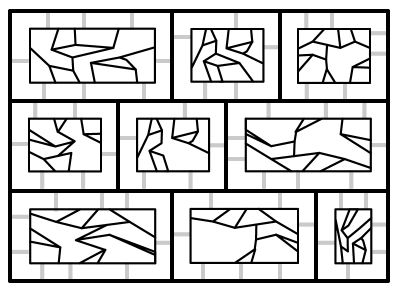
The algorithm for computing MG first computes a 2-approximate Steiner tree [21, 26, 28] and then augments this subgraph with short paths. The resulting graph is a grid-like subgraph (the bold edges in Figure 5(a)) many of whose subpaths are $\epsilon$ -short:

Definition 4.1.

A path $P$ in a graph $G$ is $\epsilon$ -short if for every pair of vertices $x$ and $y$ on $P$ ,

{dist}_{P}(x,y)\leq(1+\epsilon){dist}_{G}(x,y).

That is, the distance from $x$ to $y$ along $P$ is at most $(1+\epsilon)$ times the distance from $x$ to $y$ in $G$ .

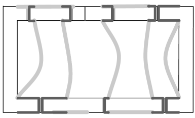
For each face $f$ of the mortar graph, the subgraph of $G$ enclosed by that face (including the edges and vertices of the face boundary) is called a brick (Figure 5(b)), and the brick’s boundary is defined to be $f$ . The boundary of a brick $B$ is written $\partial B$ . The interior of $B$ is defined to be the subgraph of edges of $B$ not belonging to $\partial B$ . The interior of $B$ is written $\text{int}(B)$ .

Bricks satisfy the following:

Lemma 4.2 (Lemma 6.10 [9]).

The boundary of a brick $B$ , in counterclockwise order, is the concatenation of four paths $W_{B},S_{B},E_{B},N_{B}$ (west, south, east, north) such that:

1.

The set of edges $B-\partial B$ is nonempty.
2.

Every vertex of $Q\cap B$ is in $N_{B}$ or in $S_{B}$ .
3.

$N_{B}$ is 0-short in $B$ , and every proper subpath of $S_{B}$ is $\epsilon$ -short in $B$ .
4.

There exists a number $t\leq\kappa(\epsilon)$ and vertices $s_{0},s_{1},s_{2},\ldots,s_{t}$ ordered from west to east along $S_{B}$ such that, for any vertex $x$ of $S_{B}[s_{i},s_{i+1})$ , the distance from $x$ to $s_{i}$ along $S_{B}$ is less than $\epsilon$ times the distance from $x$ to $N_{B}$ in $B$ : ${dist}_{S_{B}}(x,s_{i})<\epsilon\,{dist}_{B}(x,N_{B})$ .

The number $\kappa(\epsilon)$ is given by:

\kappa(\epsilon)=4\epsilon^{−2}(1+\epsilon^{−1})

(2)

The mortar graph has some additional properties. Let $B_{1}$ be a brick, and suppose $B_{1}$ ’s eastern boundary $E_{B_{1}}$ contains at least one edge. Then there is another brick $B_{2}$ whose western boundary $W_{B_{2}}$ exactly coincides with $E_{B_{1}}$ . Similarly, if $B_{2}$ is a brick whose western boundary contains at least one edge then there is a brick $B_{1}$ whose eastern boundary coincides with $B_{2}$ ’s western boundary.

The paths forming eastern and western boundaries of bricks are called supercolumns.

Lemma 4.3 (Lemma 6.6 [9]).

The sum of the costs of the edges in supercolumns is at most $\epsilon\,{\rm OPT}$ .

The mortar graph and the bricks are building blocks of the structural properties required for designing an approximation scheme. Borradaile, Klein and Mathieu demonstrated that there is a near-optimal Steiner tree whose interaction with the mortar graph is “simple” [9]. We prove a similar theorem in Section 5. In order to formalize the notion of “simple”, we select a subset of vertices on the boundary of each brick, called portals, and define a portal-connected graph.

4.2 Portals and simple connections

We define a subset of $\theta$ evenly spaced vertices along the boundary of every brick. The value of $\theta$ depends polynomially on the precision $\epsilon$ and on $\alpha$ , a parameter that represents how complex the solution can be within a single brick ( $\alpha$ will be defined precisely in Equation (6))

\theta(\epsilon)\mbox{ is }O(\epsilon^{-2}\alpha(\epsilon))

(3)

The portals are selected to satisfy the following:

Lemma 4.4 (Lemma 7.1 [9]).

For any vertex $x$ on $\partial B$ , there is a portal $y$ such that the cost of the $x$ -to- $y$ subpath of $\partial B$ is at most $1/\theta$ times the cost of $\partial B$ .

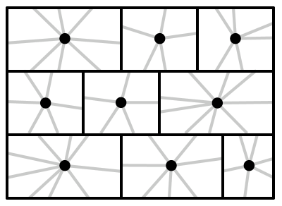
Recall that, for each face $f$ of the mortar graph $MG$ , there is a corresponding brick $B$ , and that $B$ includes the vertices and edges comprising the boundary of $f$ . The next graph construction starts with the disjoint union of the mortar graph $MG$ with all the bricks. Each edge $e$ of the mortar graph is represented by three edges in the disjoint union: one in $MG$ (the mortar-graph copy of $e$ ) and one on each of two brick boundaries (the brick copies of $e$ ). Similarly, each vertex on the boundary of a brick occurs several times in the disjoint union.

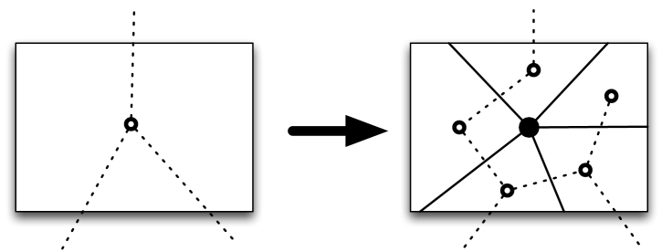
The portal-connected graph, denoted ${\cal B}^{+}(MG)$ , is obtained from the disjoint union as follows: a copy of each brick $B$ of $MG$ is embedded in the interior of the corresponding face of $MG$ , and each portal $p$ of $B$ is connected by an artificial edge to the corresponding vertex of $MG$ . The construction is illustrated in Figure 5(c). The artificial edges are called portal edges, and are assigned zero cost.

Noting that each vertex $v$ on the boundary of a brick occurs several times in ${\cal B}^{+}(MG)$ , we identify the original vertex $v$ of $G$ with that duplicate in ${\cal B}^{+}(MG)$ that belongs to $MG$ . In particular, each terminal (vertex in $Q$ ) is considered to appear exactly once in ${\cal B}^{+}(MG)$ , namely in $MG$ . Thus the original instance gives rise to an instance in ${\cal B}^{+}(MG)$ : the goal is to compute the optimal solution w.r.t. the terminals on $MG$ in ${\cal B}^{+}(MG)$ and then map the edges of this solution to $G$ . Since $G$ can be obtained from ${\cal B}^{+}(MG)$ by contracting portal edges and identifying all duplicates of each edge and all duplicates of each vertex, we infer:

Lemma 4.5.

Let $H$ be a subgraph of ${\cal B}^{+}(MG)$ that, for each pair of terminals $u,v$ , contains at least $\min\{r(u),r(v)\}$ edge-disjoint $u$ -to- $v$ paths. Then the subgraph of $G$ consisting of edges of $H$ that are in $G$ has the same property.

The graph ${\cal B}^{\div}(MG)$ , which we call the brick-contracted graph, is obtained by contracting each brick in ${\cal B}^{+}(MG)$ to a single vertex, called a brick vertex, as illustrated in Figure 5(d). This graph will be used in designing the dynamic program in Section 6.

4.3 Structure Theorem

Lemma 4.5 implies that, to find an approximately optimal solution in $G$ , it suffices to find a solution in ${\cal B}^{+}(MG)$ whose cost is not much more than the cost of the optimal solution in $G$ . The following theorem, which we prove in Section 5, suggests that this goal is achievable. An equivalent theorem was proven for the Steiner tree problem [9].

Theorem 4.6 (Structure Theorem).

For any $\epsilon>0$ and any planar instance $(G,\bm{r})$ of the $\{0,1,2\}$ -edge connectivity problem, there exists a feasible solution $S$ to the corresponding instance $({\cal B}^{+}(MG),\bm{r})$ such that

•

the cost of $S$ is at most $(1+c\epsilon){\rm OPT}$ where $c$ is an absolute constant, and
•

the intersection of $S$ with any brick $B$ is the union of a set of non-crossing trees whose leaves are portals.

4.4 Approximation scheme

We assume that the input graph $G$ has degree at most three. This can be achieved using a well-known embedding-preserving transformation in which each vertex of degree $d>3$ is replaced with a cycle of $d$ degree-three vertices, as shown in Figure 6. Making this assumption simplifies the dynamic program using for Step 5 below.

The approximation scheme consists of the following steps.

Step 1:

Find the mortar graph MG.
Step 2:
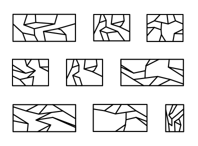
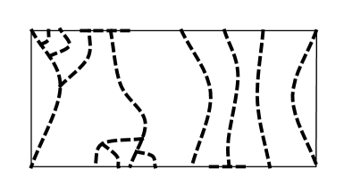
Decompose MG into “parcels”, subgraphs with the following properties:
1. (a)
  
  The parcels partition the faces of MG. Since each edge of MG belongs to the boundaries of exactly two faces, it follows that each edge belongs to at most two parcels.
2. (b)
  
  The cost of all boundary edges (those edges belonging to two parcels) is at most $\frac{1}{\eta}\bm{c}(\text{\it MG})$ . We choose $\eta$ so that this bound is $\frac{\epsilon}{2}\bm{c}(OPT)$ :
  
  $\eta=\eta(\epsilon)=\lceil 20\epsilon^{-2}\rceil$ (4)
3. (c)
  
  The planar dual of each parcel has a spanning tree of depth at most $\eta+1$ .
Each parcel $P$ corresponds to a subgraph of $G$ , namely the subgraph consisting of the bricks corresponding to the faces making up $P$ . Let us refer to this subgraph as the filled-in version of $P$ .
Step 3:
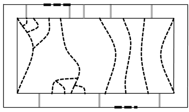
Select a set of “artificial” terminals on the boundaries of parcels to achieve the following:
- •
  
  for each filled-in parcel, there is a solution that is feasible with respect to original and artificial terminals whose cost is at most that of the parcel’s boundary plus the cost of the intersection of OPT with the filled-in parcel, and
- •
  
  the union over all parcels of such feasible solutions is a feasible solution for the original graph.
Step 4:

Designate portals on the boundary of each brick.
Step 5:

For each filled-in parcel $P$ , find a optimal solution in the portal-connected graph, ${\cal B}^{+}(P)$ . Output the union of these solutions.

Step 1 can be carried out in $O(n\log n)$ time [9]. Step 2 can be done in linear time via breadth-first search in the planar dual of MG, and then applying a “shifting” technique in the tradition of Baker [1]. Step 3 uses the fact that each parcel’s boundary consists of edge-disjoint, noncrossing cycles. If such a cycle separates terminals, a vertex $v$ on the cycle is designated an artificial terminal. We set $r(v)=2$ if the cycle separates terminals with requirement 2 and $r(v)=1$ otherwise. Under this condition, any feasible solution for the original graph must cross the cycle; by adding the edges of the cycle, we get a feasible solution that also spans the artificial terminal. Step 3 can be trivially implemented in linear time. Step 5 is achieved in linear time using dynamic programming (Section 6).

5 Proof of the Structure Theorem

We are now ready to prove the Structure Theorem for $\{0,1,2\}$ -edge connectivity, Theorem 4.6. In order to formalize the notion of connectivity across the boundary of a brick, we use the following definition:

Definition 5.1 (Joining vertex).

Let $H$ be a subgraph of $G$ and $P$ be a subpath of $\partial G$ . A joining vertex of $H$ with $P$ is a vertex of $P$ that is the endpoint of an edge of $H-P$ .

We will use the following structural lemmas in simplifying ${\rm OPT}$ . The first two were used in proving a Structure Theorem for the Steiner tree PTAS [9]; in these, $T$ is a tree and $P$ is an $\epsilon$ -short path on the boundary of the graph in which $T$ and $P$ are embedded. The third is in fact a generalization of the second lemma that we require for maintaining two connectivity.

Lemma 5.2 (Simplifying a tree with one root, Lemma 10.4 [9]).

Let $r$ be a vertex of $T$ . There is another tree $\widehat{T}$ that spans $r$ and the vertices of $T\cap P$ such that $\bm{c}(\widehat{T})\leq(1+4\cdot\epsilon)\bm{c}(T)$ and $\widehat{T}$ has at most $11\cdot\epsilon^{-1.45}$ joining vertices with $P$ .

Lemma 5.3 (Simplifying a tree with two roots, Lemma 10.6 [9]).

Let $p$ and $q$ be two vertices of $T$ . There is another tree $\widehat{T}$ that spans $p$ and $q$ and the vertices of $T\cap P$ such that $\bm{c}(\widehat{T})\leq(1+c_{1}\epsilon)\bm{c}(T)$ and $\widehat{T}$ has at most $c_{2}\cdot\epsilon^{-2.5}$ joining vertices with $P$ , where $c_{1}$ and $c_{2}$ are constants.

Lemma 5.4.

Let $\mathcal{F}$ be a set of non-crossing trees whose leaves are vertices of $\epsilon$ -short boundary paths $P$ and $Q$ and such that each tree in the forest has leaves on both these paths. There is a cycle or empty set $\widehat{C}$ , a set $\widehat{\mathcal{F}}$ of trees, and a mapping $\phi:\mathcal{F}\longrightarrow\widehat{\mathcal{F}}\cup\{\widehat{C}\}$ with the following properties

•

For every tree $T$ in $\mathcal{F}$ , $\phi(T)$ spans $T$ ’s leaves.
•

For two trees $T_{1}$ and $T_{2}$ in $F$ , if $\phi(T_{i})\neq\widehat{C}$ for at least one of $i=1,2$ then $\phi(T_{1})$ and $\phi(T_{2})$ are edge-disjoint (taking into account edge multiplicities).
•

The subgraph $\bigcup\widehat{\mathcal{F}}\cup\{\widehat{C}\}$ has $o(\epsilon^{-2.5})$ joining vertices with $P\cup Q$ .
•

$\bm{c}(\widehat{C})+\sum\{\bm{c}(T)\ :\ T\in\widehat{\mathcal{F}}\}\leq 3\bm{c}(Q)+(1+d\cdot\epsilon)\sum\{\bm{c}(T)\ :T\in\mathcal{F}\}$ where $d$ is an absolute constant.

Proof.

View the embedding of the boundary such that $P$ is on top and $Q$ is at the bottom. Let $T_{1},\ldots,T_{k}$ be the trees of $F$ ordered according the order of their leaves from left to right.

There are two cases.

Case 1) $k>1/\epsilon$ . In this case, we reduce the number of trees by incorporating a cycle $\widehat{C}$ . Let $a$ be the smallest index such that $\bm{c}(T_{a})\leq\epsilon\bm{c}(F)$ and let $b$ be the largest index such that $\bm{c}(T_{b})\leq\epsilon\bm{c}(F)$ . We will replace trees $T_{a},T_{a+1},\ldots,T_{b}$ with a cycle. Let $Q^{\prime}$ be the minimal subpath of $Q$ that spans the leaves of $\bigcup_{i=a}^{b}T_{i}$ on $Q$ . We likewise define $P^{\prime}$ . Let $L$ be the leftmost $Q$ -to- $P$ path in $T_{a}$ and let $R$ be the rightmost $Q$ -to- $P$ path in $T_{b}$ . Since $P$ is $\epsilon$ -short,

\bm{c}(P^{\prime})\leq(1+\epsilon)\bm{c}(L\cup Q^{\prime}\cup R).

(5)

To obtain $\widehat{F}$ from $F$ , we replace the trees $T_{a},\ldots,T_{b}$ with the cycle $\widehat{C}=P^{\prime}\cup L\cup Q^{\prime}\cup R$ and set $\phi(T_{a}),\ldots,\phi(T_{b})$ to $\widehat{C}$ . By construction $\widehat{C}$ spans the leaves of $\cup_{i=a}^{b}T_{i}$ .

Case 2) $k\leq 1/\epsilon$ . In this case, the number of trees is already bounded. We set $a=2,b=1$ so as to not eliminate any trees, and we set $\widehat{C}$ to be the empty set.

In both cases, for each remaining tree $T_{i}$ ( $i\neq a,a+1,\ldots,b$ ) we do the following. Let $T_{i}^{\prime}$ be a minimal subtree of $T_{i}$ that spans all the leaves of $T_{i}$ on $P$ and exactly one vertex $r$ of $Q$ . Let $Q_{i}$ be the minimal subpath of $Q$ that spans the leaves of $T_{i}$ on $Q$ . We replace $T_{i}$ with the tree $\widehat{T}_{i}$ that is the union of $Q_{i}^{\prime}$ and the tree guaranteed by Lemma 5.2 for tree $T_{i}^{\prime}$ with root $r$ and $\epsilon$ -short path $P$ . By construction $\widehat{T}_{i}$ spans the leaves of $T_{i}$ . We set $\phi(T_{i})=\widehat{T}_{i}$ for $i\neq a,\ldots,b$ .

$\widehat{C}$ has at most four joining vertices with $P\cup Q$ . Each tree $\widehat{T}_{i}$ has one joining vertex with $Q$ and, by Lemma 5.2, $o(\epsilon^{-1.5})$ joining vertices with $P$ . By the choice of $a$ and $b$ , there are at most $2/\epsilon$ of the trees in the second part of the construction. This yields the bound on joining vertices.

The total cost of the replacement cycle is:

$\displaystyle\bm{c}(\widehat{C})$	$\displaystyle\leq$	$\displaystyle\bm{c}(P^{\prime})+\bm{c}(L)+\bm{c}(Q^{\prime})+\bm{c}(R)$
	$\displaystyle\leq$	$\displaystyle(2+\epsilon)(\bm{c}(L)+\bm{c}(Q^{\prime})+\bm{c}(R))\qquad\mbox{by Equation~\eqref{eq:1}}$
	$\displaystyle\leq$	$\displaystyle(2+\epsilon)(\bm{c}(T_{a})+\bm{c}(Q^{\prime})+\bm{c}(T_{b}))\qquad\mbox{since $L$ and $R$ are paths in $T_{a}$ and $T_{b}$}$
	$\displaystyle\leq$	$\displaystyle(2+\epsilon)(2\epsilon\bm{c}(F)+\bm{c}(Q^{\prime}))\qquad\mbox{by the choice of $a$ and $b$}$
	$\displaystyle\leq$	$\displaystyle(4\epsilon+2\epsilon^{2})\bm{c}(F)+(2+\epsilon)\bm{c}(Q^{\prime})$

The total cost of the replacement trees is:

	$\displaystyle\sum_{i=1,\ldots,a-1,b+1\ldots k}\bm{c}(\widehat{T}_{i})$	$\displaystyle\leq$	$\displaystyle\sum_{i=1,\ldots,a-1,b+1\ldots k}\bm{c}(Q_{i}^{\prime})+(1+4\epsilon)\bm{c}(T_{i}^{\prime})\qquad\mbox{by Lemma~\ref{lem:fib-tree}}$
		$\displaystyle\leq$	$\displaystyle\sum_{i=1,\ldots,a-1,b+1\ldots k}\bm{c}(Q_{i}^{\prime})+(1+4\epsilon)\bm{c}(T_{i})\qquad\mbox{since $T_{i}^{\prime}$ is a subtree of $T_{i}$}$

By the ordering of the trees and the fact that they are non-crossing, $Q^{\prime}$ and the $Q_{i}^{\prime}$ ’s are disjoint. Combining the above gives the bound on cost. ∎

5.1 Construction of a new solution

We start with a brief overview of the steps used to prove the structure theorem. We start with an edge multiset forming an optimal solution, ${\rm OPT}$ . Each step modifies either the input graph $G$ or a subgraph thereof while simultaneously modifies the solution. The graphs and edge multisets resulting from these steps are denoted by subscripts. Details are given in subsequent sections.

Augment: We add two copies of each supercolumn, obtaining $G_{A}$ and ${\rm OPT}_{A}$ . We consider the two copies to be interior to the two adjacent bricks. This step allows us, in the restructure step, to concern ourselves only with connectivity between the north and south boundaries of a brick.
Cleave: Cleaving a vertex refers to splitting it into two vertices and adding an artificial edge between the two vertices. In the cleave step, we modify $G_{A}$ (and so in turn modify $MG_{A}$ and ${\rm OPT}_{A}$ ) to create $G_{C}$ (and $MG_{C}$ and ${\rm OPT}_{C}$ ) by cleaving certain vertices while maintaining a planar embedding. Let $J_{C}$ be the set of artificial edges introduced. Note that $X_{C}/J_{C}=X_{A}$ . The artificial edges are assigned zero cost so the metric between vertices is preserved. The artificial edges are added to the solution, possibly in multiplicity, so connectivity is preserved.
Flatten: In this step, for each brick $B$ , we consider the intersection of the solution with $\text{int}(B)$ ; we replace some of the connected components of the intersection with subpaths of the boundary of $B$ . We denote the resulting solution by ${\rm OPT}_{F}$ .
Map: We map the edges of ${\rm OPT}_{F}$ to $\mathcal{B}^{+}(MG)$ creating ${\rm OPT}_{M}$ . This step temporarily disconnects the solution.
Restructure: In this step, we modify the solution ${\rm OPT}_{M}$ . For each brick $B$ in $MG_{C}$ , the part of ${\rm OPT}_{M}$ strictly interior to $B$ is replaced with another subgraph that has few joining vertices with $\partial B$ . We denote the resulting solution by ${\rm OPT}_{S}$ .
Rejoin: In order to re-establish connections broken in the Map step, we add edges to ${\rm OPT}_{S}$ . Next, we contract the artificial edges added in the cleave step. We denote the resulting solution by $\widehat{OPT}$ .

Note that the solutions ${\rm OPT}$ , ${\rm OPT}_{A}$ , and so on are multisets; an edge can occur more than once. We now describe these steps in greater detail.

5.1.1 Augment

Recall that a supercolumn is the eastern boundary of one brick and the western boundary of another, and that the sum of costs of all supercolumns is small. In the Augment step, for each supercolumn $P$ , we modify the graph as shown in Figure 7:

•

Add to the graph two copies of $P$ , called $P_{1}$ and $P_{2}$ , creating two new faces, one bounded by $P_{1}$ and $P$ and the other bounded by $P$ and $P_{2}$ .
•

Add $P_{1}$ and $P_{2}$ to ${\rm OPT}$ .

The resulting graph is denoted $G_{A}$ , and the resulting solution is denoted ${\rm OPT}_{A}^{\prime}$ . We consider $P_{1}$ and $P_{2}$ to be internal to the two bricks. Thus $P$ remains part of the boundary of each of the bricks, and $MG$ contains $P$ but not $P_{1}$ or $P_{2}$ . Since $P_{1}$ and $P_{2}$ share no internal vertices with $P$ , the joining vertices of ${\rm OPT}_{A}^{\prime}\cap B$ with $\partial B$ belong to $N_{B}$ and $S_{B}$ .

We perform one more step, a minimality-achieving step:

•

We remove edges from ${\rm OPT}_{A}^{\prime}$ until it is a minimal set of edges achieving the desired connectivity between terminals.

Let ${\rm OPT}_{A}$ be the resulting set. We get:

Lemma 5.5.

For every brick $B$ , the joining vertices of ${\rm OPT}_{A}\cap B$ with $\partial B$ belong to $N_{B}$ and $S_{B}$ .

5.1.2 Cleave

We define a graph operation, cleave. Given a vertex $v$ and a bipartition $A,B$ of the edges incident to $v$ , $v$ is cleaved by

•

splitting $v$ into two vertices, $v_{A}$ and $v_{B}$ ,
•

mapping the endpoint $v$ of edges in $A$ to $v_{A}$ ,
•

mapping the endpoint $v$ of edges in $B$ to $v_{b}$ , and
•

introducing a zero-cost edge $e_{v}=v_{A}v_{B}$ .

This operation is illustrated in Figure 8(a) and (b). If the bipartition $A,B$ is non-interleaving with respect to the embedding’s cycle of edges around $v$ then the construction maintains a planar embedding.

We use two types of cleavings:

Simplifying cleavings: Refer to Figures 8(c) and (d). Let $C$ be a clockwise non-self-crossing, non-simple cycle that visits vertex $v$ twice. Define a bipartition $A,B$ of the edges incident to $v$ as follows: given the clockwise embedding of the edges incident to $v$ , let $A$ start and end with consecutive edges of $C$ and contain only two edges of $C$ . Such a bipartition exists because $C$ is non-self-crossing.
Lengthening cleavings: Refer to Figures 8(e) and (f). Let $C$ be a cycle, let $v$ be a vertex on $C$ with two edges $e_{A}$ and $e_{B}$ adjacent to $v$ embedded strictly inside $C$ , and let $e_{A}^{\prime}$ and $e_{B}^{\prime}$ be consecutive edges of $C$ adjacent to $v$ such that the following bipartition is non-crossing with respect to the embedding: $A,B$ is a bipartition of the edges adjacent to $v$ such that $e_{A},e_{A}^{\prime}\in A$ and $e_{B},e_{B}^{\prime}\in B$ .

We perform simplifying cleavings for non-simple cycles of ${\rm OPT}_{A}$ until every cycle is simple; the artificial edges introduced are not included in ${\rm OPT}$ . The following lemma does not use planarity and shows that (since cycles get mapped to cycles in this type of cleaving) simplifying cleavings preserve two-edge connectivity.

Lemma 5.6.

Let $e$ be an edge in a graph $H$ . Let $\widehat{H}$ be the graph obtained from $H$ by a simplifying cleaving. Then $e$ is a cut-edge in $H$ iff it is a cut-edge in $\widehat{H}$ .

Proof.

Let $u_{1},u_{2}$ be the endpoints of $e$ and let $C$ be the cycle w.r.t. which a simplifying cleaving was performed. If $H$ contains an $e$ -avoiding $u_{i}$ -to- $C$ path for $i=1,2$ then $e$ is not a cut-edge in $H$ , and similarly for $\widehat{H}$ . Suppose therefore that removing $e$ separates $u_{i}$ from $C$ in $H$ . Then the same is true in $\widehat{H}$ , and conversely. ∎

Corollary 5.7.

For $k=1,2$ , if two vertices are $k$ -edge connected in $H$ then any of their copies are $k$ -edge connected in $H_{C}$ .

Moreover, after all the simplifying cleavings, every cycle is simple, so:

Lemma 5.8.

Vertices that are two-edge-connected in ${\rm OPT}_{C}$ are biconnected.

Next we perform lengthening cleavings w.r.t. the boundary of a brick and edges $e_{A}$ and $e_{B}$ of ${\rm OPT}_{C}$ ; we include in ${\rm OPT}_{C}$ all the artificial zero-cost edges introduced. Lengthening cleavings clearly maintain connectivity. Suppose that vertices $x$ and $y$ are biconnected in ${\rm OPT}_{C}$ , and consider performing a lengthening cleaving on a vertex $v$ . Since there are two internally vertex-disjoint $x$ -to- $y$ paths in ${\rm OPT}_{C}$ , $v$ cannot appear on both of them. It follows that there remain two internally vertex-disjoint $x$ -to- $y$ paths after the cleaving. We obtain the following lemma.

Lemma 5.9.

Lengthening cleavings maintain biconnectivity.

Lengthening cleavings are performed while there are still multiple edges of the solution embedded in a brick that are incident to a common boundary vertex. Let $J_{C}$ be the set of artificial edges that are introduced by simplifying and lengthening cleavings. We denote the resulting graph by $G_{C}$ , we denote the resulting mortar graph by $MG_{C}$ , and we denote the resulting solution by ${\rm OPT}_{C}$ .

As a result of the cleavings, we get the following:

Lemma 5.10.

Let $B$ be a brick in $G_{C}$ with respect to $MG_{C}$ . The intersection ${\rm OPT}_{C}\cap\text{int}(B)$ is a forest whose joining vertices with $\partial B$ are the leaves of the forest.

Proof.

Let $H$ be a connected component of ${\rm OPT}_{C}\cap\text{int}(B)$ . As a result of the lengthening cleavings, the joining vertices of $H$ with $\partial B$ have degree 1 in $H$ . Suppose otherwise; then there is a vertex $v$ of $H\cap\partial B$ that has degree $>1$ in $H$ . Hence $v$ is a candidate for a lengthening cleaving, a contradiction.

By Theorem 2.5 and the minimality-achieving step of the Augment step, any cycle in $H$ must include a terminal $u$ with $r(u)=2$ by Theorem 2.5. Since there are no terminals strictly enclosed by bricks, $u$ must be a vertex of $\partial B$ . However, that would make $u$ a joining vertex of $H$ with $\partial B$ . As argued above, such vertices are leaves of $H$ , a contradiction to the fact that $u$ is a vertex of a cycle in $H$ . Therefore $H$ is acyclic.

Furthermore, leaves of $H$ are vertices of $\partial B$ since ${\rm OPT}_{C}$ is minimal with respect to edge inclusion and terminals are not strictly internal to bricks. ∎

Lemma 5.11.

Let $C$ be a cycle in ${\rm OPT}_{C}$ . Let $B$ be a brick. Distinct connected components of $C\cap\text{int}(B)$ belong to distinct components of ${\rm OPT}_{C}\cap\text{int}(B)$ .

Proof.

Assume the lemma does not hold. Then there is a $C$ -to- $C$ path $P$ in $\text{int}(B)$ . Each vertex of $P$ that is strictly interior to $B$ is not a terminal. A vertex of $P$ that was on $\partial(B)$ would be a candidate for a lengthening cleaving, a contradiction. Therefore $P$ includes no terminals. This contradicts Theorem 2.6. ∎

5.1.3 Flatten

For each brick $B$ , consider the edges of ${\rm OPT}_{C}$ that are strictly interior to $B$ . By Lemma 5.10, the connected components are trees. By Lemma 5.5, for each such tree $T$ , every leaf is either on $B$ ’s northern boundary $N_{B}$ or on $B$ ’s southern boundary $S_{B}$ . For each such tree $T$ whose leaves are purely in $N_{B}$ , replace $T$ with the minimal subpath of $N_{B}$ that contains all the leaves of $T$ . Similarly, for each such tree $T$ whose leaves are purely in $S_{B}$ , replace $T$ with the minimal subpath of $S_{B}$ that contains all the leaves of $T$ .

Let ${\rm OPT}_{F}$ be the resulting solution. Note that ${\rm OPT}_{F}$ is a multiset. An edge of the mortar graph can appear with multiplicity greater than one.

5.1.4 Map

This step is illustrated in Figures 9(a) and (b). In this step, the multiset ${\rm OPT}_{F}$ of edges resulting from the flatten step is used to select a set ${\rm OPT}_{M}$ of edges of ${\cal B}^{+}(MG_{C})$ . Recall that every edge $e$ of $MG_{C}$ corresponds in ${\cal B}^{+}(MG_{C})$ to three edges: two brick copies (one in each of two bricks) and one mortar-graph copy. In this step, for every edge $e$ of $MG_{C}$ , we include the mortar-graph copy of $e$ in ${\rm OPT}_{M}$ with multiplicity equal to the multiplicity of $e$ in ${\rm OPT}_{F}$ . At this point, none of the brick copies are represented in ${\rm OPT}_{M}$ .

Next, recall that in the augment step, for each supercolumn $P$ , we created two new paths, $P_{1}$ and $P_{2}$ , and added them to ${\rm OPT}$ . The edges of these two paths were not considered part of the mortar graph, so mortar-graph copies were not included in ${\rm OPT}_{M}$ for these edges. Instead, for each such edge $e$ , we include the brick-copy of $e$ in ${\rm OPT}_{F}$ with multiplicity equal to the multiplicity of $e$ in ${\rm OPT}_{F}$ .

Finally, for each edge $e$ interior to a brick, we include $e$ in ${\rm OPT}_{M}$ with the same multiplicity as it has in ${\rm OPT}_{F}$ .

5.1.5 Restructure

Let $B$ be a brick. For simplicity, we write the boundary paths of $B$ as $N,E,S,W$ . Let $F$ be the multiset of edges of ${\rm OPT}_{M}$ that are in the interior of $B$ . $F$ is a forest (Lemma 5.10). As a result of the flatten step, each component of $F$ connects $S$ to $N$ . We will replace $F$ with another subgraph $\widehat{F}$ and map each component $T$ of $F$ to a subgraph $\phi(T)$ of $\widehat{F}$ where $\phi(T)$ spans the leaves of $T$ and is a tree or a cycle. Distinct components of $F$ are mapped by $\phi$ to edge-disjoint subgraphs (taking into account multiplicities).

Refer to Figure 10. We inductively define $S$ -to- $N$ paths $P_{0},P_{1},\ldots$ and corresponding integers $k_{0},k_{1},\ldots$ . Let $s_{0},\ldots,s_{t}$ be the vertices of $S$ guaranteed by Lemma 4.2 (where $s_{0}$ is the vertex common to $S$ and $W$ and $s_{t}$ is the vertex common to $S$ and $E$ ). Let $P_{0}$ be the easternmost path in $F$ from $S$ to $N$ . Let $k_{0}$ be the integer such that $\text{start}(P_{0}))$ is in $S[s_{k_{0}},s_{k_{0}+1})$ . Inductively, for $i\geq 0$ , let $P_{i+1}$ be the easternmost path in $F_{N\wedge S}$ from $S[s_{0},s_{k_{i}})$ to $N$ that is vertex-disjoint from $P_{i}$ . Let $k_{i}$ be the integer such that $\text{start}(P_{i})\in S[s_{k_{i}},s_{k_{i}+1})$ . This completes the inductive definition of $P_{0},P_{1},\ldots$ . Note that the number of paths is at most $t$ , which in turn is at most $\kappa(\epsilon)$ as defined in Equation 2.

We use these paths to decompose $F$ , as illustrated in Figure 10. Let $F_{i}$ be the set of edges of $F-P_{i+1}$ enclosed by the cycle formed by $P_{i}$ , $P_{i+1}$ , $N$ and $S$ . Clearly $F=\cup_{i}F_{i}$ . If $P_{i}$ is connected to $P_{i+1}$ , they share at most one vertex, $w_{i}$ . If they are not connected, we say $w_{i}$ is undefined.

There are two cases: either $F_{i}$ is connected or not.

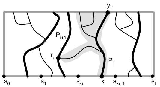
Connected case:

There are two subcases. Either $F_{i}$ spans vertices of $S[\cdot,s_{k_{i}})$ or not.

Suppose $F_{i}$ spans vertices of $S[\cdot,s_{k_{i}})$ . Let $T_{S}$ be a minimal subtree of $F_{i}$ that spans $F_{i}\cap S$ and let $T_{N}$ be a minimal subtree of $F_{i}$ that spans $F_{i}\cap N$ . Let $r_{N}$ be the first vertex of $P_{i}$ in $T_{N}$ and let $r_{S}$ be the last vertex of $P_{i}$ in $T_{S}$ . A path in $F_{i}$ from $T_{S}$ to $N$ that does not go through $r_{S}$ contradicts the choice of $P_{i+1}$ as there would be a path in $F_{i}$ from $S[\cdot,s_{k_{i}})$ to $N$ that is disjoint from $P_{i}$ . It follows that $T_{S}$ and $T_{N}$ are edge disjoint: if they intersect they may only do so at $r_{S}=r_{N}$ . If $w_{i}$ is defined, then there is a path $Q$ from $w_{i}$ to $P_{i}$ ; $Q$ intersects $P_{i}$ between $r_{N}$ and $r_{S}$ , for otherwise there would be a superpath of $Q$ that contradicts the choice of $P_{i+1}$ .

If $w_{i-1}$ is defined and $w_{i-1}\in T_{N}$ , then we replace $T_{N}$ with the tree guaranteed by Lemma 5.3 with roots $r_{N}$ and $w_{i-1}$ . Otherwise, we replace $T_{N}$ with the tree guaranteed by Lemma 5.2 with root $r_{N}$ . We do the same for $T_{S}$ .

Suppose $F_{i}$ does not span vertices of $S[\cdot,s_{k_{i}})$ . Let $T_{N}$ be a minimal connected subgraph of $F_{i}\cup S[s_{k_{i}},\text{start}(P_{i})]$ that spans $F_{i}\cap N$ . Let $r_{N}$ be the first vertex of $P_{i}$ in $T_{N}$ . If $w_{i}$ is defined, then there is a path $Q$ from $w_{i}$ to $P_{i}\cup S[s_{k_{i}},\text{start}(P_{i})]$ and $Q$ ’s intersection with $P_{i}$ belongs to $P_{i}[\cdot,r_{N}]$ , for otherwise there would be a superpath of $Q$ that contradicts the choice of $P_{i+1}$ . If $w_{i-1}$ is defined and $w_{i-1}\in T_{N}$ , then we replace $F_{i}$ with the tree guaranteed by Lemma 5.3 with roots $r_{N}$ and $w_{i-1}$ along with $Q$ , $P_{i}[\cdot,r_{N}]$ , and $S[s_{k_{i}},\text{start}(P_{i})]$ . Otherwise we replace $F_{i}$ with the tree guaranteed by Lemma 5.2 with root $r_{N}$ along with $Q$ , $P_{i}[\cdot,r_{N}]$ , and $S[s_{k_{i}},\text{start}(P_{i})]$ .

In both cases, we define $\phi^{\prime}(F_{i})$ to be the resulting tree that replaces $F_{i}$ . By construction, $\phi^{\prime}(F_{i})$ spans the leaves of $F_{i}$ and $w_{i-1}$ and $w_{i}$ (if defined).

Disconnected case:

In this case, by the definition of $P_{i+1}$ , $F_{i}\cap S$ is a subset of the vertices of $S[s_{k_{i}},\text{start}(P_{i})]$ , for otherwise there would be a path to the right of $P_{i+1}$ that connects to $N$ and is disjoint from $P_{i}$ .

If $F_{i}$ is connected to $F_{i+1}$ , then the western-most tree $T_{W}$ is a tree with root $w_{i}$ and leaves on $S$ and does not connect to $N$ as that would contradict the choice of $P_{i+1}$ ; if this is the case, let $\widehat{T}_{W}$ be the tree guaranteed by Lemma 5.2 and define $\phi^{\prime}(T_{W})=\widehat{T}_{W}$ .

If $F_{i}$ is connected to $F_{i-1}$ , let $S^{\prime}$ be the subpath of $S$ that spans the eastern-most tree $T_{E}$ ’s leaves on $S$ . Let $\widehat{T}_{E}$ be the tree guaranteed by Lemma 5.3 that spans the eastern-most tree’s leaves on $N$ and roots $w_{i-1}$ and $\text{start}(P_{i})$ and define $\phi^{\prime}(T_{E})=\widehat{T}_{E}$ .

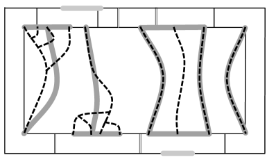
Let $\mathcal{F}$ be the set of remaining trees, let $P=N$ , and let $Q=S[s_{k_{i}},\text{start}(P_{i})]$ in Lemma 5.4. Let $\widehat{C}$ , $\widehat{\mathcal{F}}$ , and $\phi$ be the cycle (or empty set), set of trees, and mapping that satisfy the properties stated in the lemma.

We define $\widehat{F}_{i}$ to consist of the trees of $\widehat{\mathcal{F}}$ and the cycle $\widehat{C}$ (and $\widehat{T}_{W}$ , $S^{\prime}$ and $\widehat{T}_{E}$ if defined).

We replace every $F_{i}$ with $\widehat{F}_{i}$ , as described above, for every brick, creating ${\rm OPT}_{S}$ . This is illustrated in Figure 11(a). Now we define $\phi$ in terms of $\phi^{\prime}$ . A component $T$ of $F$ is partitioned into adjacent trees in this restructuring: namely $T_{1},\ldots,T_{k}$ , $k\geq 1$ . $T_{1}$ and $T_{k}$ may be restructured via the disconnected case and all others are restructured via the connected case. Define $\phi(T)=\cup_{i=1}^{k}\phi^{\prime}(T_{i})$ . If $k>1$ , then consecutive trees $T_{i}$ and $T_{i+1}$ share a vertex $w_{i}$ and by construction $\phi^{\prime}(T_{i})$ and $\phi^{\prime}(T_{i})$ also share this vertex. Since $\phi^{\prime}(T)$ spans the leaves of $T$ , we get that $\phi(T)$ spans the leaves of $T$ , as desired. Also by construction, the submapping of $\phi^{\prime}$ of trees to trees (and not cycles) is bijective; the same holds for $\phi$ .

Number of joining vertices

In both the connected and disconnected case, the number of leaves is the result of a constant number of trees resulting from Lemmas 5.2, 5.3 and 5.4. Therefore, $\widehat{F}_{i}$ has $o(\epsilon^{-2.5})$ joining vertices with $N$ and $S$ . Since $i\leq\kappa(\epsilon)=O(\epsilon^{-3})$ , ${\rm OPT}_{S}$ has $o(\epsilon^{-5.5})$ joining vertices with the boundary of each brick. This is the number of connections required to allow a solution to be nearly optimal and affects the number of portals required in Equation (3):

\alpha(\epsilon)\mbox{ is }o(\epsilon^{-5.5})

(6)

This will allow us to prove the second part of the Structure Theorem.

5.1.6 Rejoin

In this step, we make inter-brick connections for parts that were disconnected in the mapping step. Since joining vertices represent the ends of all disconnected parts, it suffices to connect joining vertices of ${\rm OPT}_{S}$ with $\partial B$ to their mortar-graph counterparts via portal edges.

This is illustrated in Figure 11 (d): We first move the edges of ${\rm OPT}_{S}\cap\partial B$ to $MG$ for every brick $B$ . Such edges may have been introduced in the restructure step: for every brick $B$ , we connect ${\rm OPT}_{S}\cap B$ to the mortar graph. For every joining vertex $v$ of ${\rm OPT}_{S}\cap B$ , we find the nearest portal $p_{v}$ , add the subpath of $\partial B$ and $MG$ connecting $v$ and $p_{v}$ and add the portal edge corresponding to $p_{v}$ . (We need at most two copies of each portal edge.) Finally we contract the edges introduced in the cleaving step. This produces a solution $\widehat{OPT}$ of $\mathcal{B}^{+}(MG)$ .

5.2 Analysis of connectivity

In the augment step, because the added paths $P_{1}$ and $P_{2}$ form a cycle, this transformation preserves two-connectivity and connectivity between terminals. Cleaving clearly preserves connectivity and, by Lemmas 5.8 and 5.9, terminals that require two-connectivity are biconnected in ${\rm OPT}_{C}$ . Therefore, for terminals $x$ and $y$ requiring connectivity, there is a path $P_{C}$ in ${\rm OPT}_{C}$ connecting them. If $x$ and $y$ require two-connectivity, there is a simple cycle $C_{C}$ in ${\rm OPT}_{C}$ connecting them. We follow $P_{C}$ and $C_{C}$ through the remaining steps.

Flatten: Consider a tree $T$ that is replaced by a subpath $Q$ of a northern or southern boundary of a brick that spans $T$ ’s leaves. $Q$ spans any terminals that $T$ spanned, since there are no terminals internal to bricks.

$P_{C}\cap T$ is therefore a (set of) leaf-to-leaf paths and so $(P_{C}-T)\cup Q$ contains an $x$ -to- $y$ path. It follows that there is an $x$ -to- $y$ path $P_{F}$ in ${\rm OPT}_{F}$ .

By Lemma 5.11, $C_{C}\cap T$ is a single path and, by the above reasoning, is a leaf-to-leaf path. Therefore $(C_{C}-T)\cup Q$ contains a cycle through $x$ and $y$ . It follows that there is a cycle $C_{F}$ through $x$ and $y$ in ${\rm OPT}_{F}$
Map: $P_{F}$ ( $C_{F}$ ) gets mapped to a sequence ${\cal P}_{M}=(P_{M}^{1},P_{M}^{2},\ldots)$ , (a cyclic sequence ${\cal C}_{M}=(C_{M}^{1},C_{M}^{2},\ldots)$ ) of paths of ${\rm OPT}_{M}$ in ${\cal B}^{+}(MG_{C})$ such that each path either consists completely of mortar-graph edges or consists completely of brick-copy edges. The last vertex of one path and the first vertex of the next path are copies of the same vertex of $G_{C}$ , and that vertex belongs to a north or south boundary of $MG_{C}$ . By Lemma 5.10, each path in ${\cal P}_{M}$ or ${\cal C}_{M}$ that consists of brick-copy edges starts and ends at the northern or southern boundary of a brick.
Restructure: We define a mapping $\hat{\phi}$ , based in part on the map $\phi$ defined in Section 5.1.5. For a path $Q$ in ${\cal P}_{M}$ or ${\cal C}_{M}$ that uses mortar-copy edges, define $\hat{\phi}(Q)=Q$ . For a path $Q$ in ${\cal P}_{M}$ or ${\cal C}_{M}$ that uses brick-copy edges, let $T$ be the tree in ${\rm OPT}_{M}$ that contains $Q$ and define $\hat{\phi}(Q)=\phi(T)$ .

Let ${\cal C}_{S}$ be the cyclic sequence of trees and cycles to which ${\cal C}_{M}$ maps by $\phi$ . Since $\phi(T)$ spans the leaves (joining vertices) of $T$ , consecutive trees/cycles in ${\cal C}_{S}$ contain copies of the same vertex. By Lemma 5.11 and that, within a brick, the preimage of the set of trees mapped to by $\phi$ , the trees of ${\cal C}_{S}$ are edge disjoint. (The cycles may be repeated.)

Likewise we define ${\cal P}_{S}$ having the same properties except for the fact that the sequence is not cyclic.
Rejoin: This step reconnects ${\cal P}_{S}$ and ${\cal C}_{S}$ .

Consider a tree $T$ in either of these sequences that contains brick-copy edges. The rejoin step first moves any edge of $T$ that is in a brick boundary to the mortar copy. It then connects joining vertices to the mortar by way of detours to portals and portal edges. Therefore, $T$ is mapped to a tree $T_{J}$ that connects the mortar copies of $T$ ’s leaves.

Consider a cycle $C$ in either ${\cal P}_{S}$ or ${\cal C}_{S}$ . $C$ contains a subpath of $N$ and $S$ whose edges are moved to their mortar copy and two $N$ -to- $S$ paths whose joining vertices are connected to their mortar copies. Therefore $C$ is mapped to a cycle $C_{J}$ through the mortar copies of the boundary vertices of $C$ .

Let the resulting sequence and cyclic sequence of trees and cycles be ${\cal P}_{J}$ and ${\cal C}_{J}$ . Since consecutive trees/cycles in ${\cal C}_{S}$ contain copies of the same vertex, in ${\cal C}_{J}$ consecutive trees/cycles contain common mortar vertices. We have that ${\cal C}_{J}$ is a cyclic sequence of trees and cycles, through $x$ and $y$ , the trees of which are edge-disjoint. Therefore the union of these contains a cycle through $x$ and $y$ .

Similarly, we argue that the union of the trees and cycles in ${\cal P}_{J}$ contains and $x$ -to- $y$ path.

5.3 Analysis of cost increase

By Lemma 4.3, the total costs of all the east and west boundaries of the bricks is an $\epsilon$ fraction of ${\rm OPT}$ , so we have

\bm{c}({\rm OPT}_{A})\leq(1+2\epsilon)\bm{c}({\rm OPT}).

(7)

The cleaving step only introduces edges of zero cost, so

\bm{c}({\rm OPT}_{C})=\bm{c}({\rm OPT}_{A}).

(8)

The flatten step replaces trees by $\epsilon$ -short paths, and so can only increase the cost by an $\epsilon$ fraction, giving:

\bm{c}({\rm OPT}_{F})\leq(1+\epsilon)\bm{c}({\rm OPT}_{C}).

(9)

The mapping step does not introduce any new edges, so

\bm{c}({\rm OPT}_{M})=\bm{c}({\rm OPT}_{F}).

(10)

The restructure step involves replacing disjoint parts of ${\rm OPT}_{M}\cap B$ for each brick by applying Lemmas 5.2, 5.3, and 5.4. This increases the cost of the solution by at most an $O(\epsilon)$ fraction. Further we add subpaths of $S[s_{k_{i}},\text{start}(P_{i})]$ where ${\rm OPT}_{M}$ contains disjoint subpaths $P_{i}$ from $\text{start}(P_{i})$ to $N$ and by the brick properties, $\bm{c}(S[s_{k_{i}},\text{start}(P_{i})])\leq\bm{c}(P_{i})$ . This increases the the cost of the solution by at most another $O(\epsilon)$ fraction. We get, for some constant $c$ :

\bm{c}({\rm OPT}_{S})\leq(1+c\epsilon)\bm{c}({\rm OPT}_{M}).

(11)

In the rejoin step, we add two paths connecting a joining vertex to its nearest portal: along the mortar graph and along the boundary of the brick. The cost added per joining vertex is at most twice the interportal cost: at most $2\bm{c}(\partial B)/\theta$ for a joining vertex with the boundary of brick $B$ , by Lemma 4.4. Since each mortar graph edge appears as a brick-boundary edge at most twice, the sum of the costs of the boundaries of the bricks is at most $18\epsilon^{-1}{\rm OPT}$ (Equation (1)). Since there are $\alpha(\epsilon)$ joining vertices of ${\rm OPT}_{S}$ with each brick, the total cost added due to portal connections is at most $36\frac{\alpha}{\theta\epsilon}{\rm OPT}$ . Replacing $\alpha$ and $\theta$ via Equations (6) and (3) gives us that the total cost added due to portal connections is

O(\epsilon\bm{c}({\rm OPT}))

(12)

Combining equations (7) through (12), $\bm{c}(\widehat{}{\rm OPT})\leq(1+c^{\prime}\epsilon)\bm{c}({\rm OPT})$ for some constant $c^{\prime}$ , proving Theorem 4.6.

6 Dynamic Program

In this section we show that there is a dynamic program that finds an approximately optimal solution in the portal-connected graph ${\cal B}^{+}(P)$ .

6.1 Structure of solution

We start by showing that we can restrict our attention to solutions whose intersection with each brick is a small collection of trees whose leaves are portals.

Lemma 6.1.

Let $S$ be a minimal solution to the instance $({\cal B}^{+}(MG),\bm{r})$ of the $\{0,1,2\}$ -edge connectivity problem. Let $B$ be a brick, and suppose that the intersection of $S$ with $B$ is the union of a set of non-crossing trees whose leaves are portals. Then the number of such trees is at most three times the number of portals.

Proof.

Let the portals be $v_{1},\ldots,v_{k}$ in counterclockwise order. Each tree induces a subpartition on the set of pairs $\{(i,i+1)\ :i\in\{1,\ldots,k-1\}\}$ as follows: if the leaves of the tree are $v_{i_{1}},v_{i_{2}},\ldots,v_{i_{p}}$ where $i_{1}<i_{2}<\cdots<i_{p}$ , then the parts are

\{(i_{1},i_{1}+1),\ldots,(i_{2}-1,i_{2})\},\{(i_{2},i_{2}+1),\ldots,(i_{3}-1,i_{3})\},\ldots,\{(i_{p-1},i_{p-1}+1),\ldots,(i_{p}-1,i_{p})\}

Because the trees are non-crossing, the corresponding subpartitions are non-crossing as well: for each pair $T_{1},T_{2}$ of trees, either each part of $T_{2}$ is a subset of some part of $T_{1}$ , or vice versa.

Therefore the trees themselves form a rooted tree $\cal T$ according to the nesting relation of the corresponding subpartitions. Furthermore, by minimality of $S$ , no three trees have the same sets of leaves. This shows that a node of $\cal T$ with only one child has a parent with at least two children. The number of leaves of $\cal T$ is at most the number of pairs $(i,i+1)$ , which is at most $k-1$ . This shows that the number of trees is at most $3(k-1)$ . ∎

Corollary 6.2.

There exists a function $f$ that maps each brick $B$ to a cardinality-at-most- $3\theta$ subpartition $f(B)$ of the portals of $B$ with the following property:
for each brick $B$ , for each part $P$ of $f(B)$ , let $T_{P}$ be any minimum-cost tree in $B$ whose leaves are $P$ , and let $H_{B}$ be the union $\bigcup_{P\in f(B)}T_{P}$ . Then there is a feasible solution $S^{\prime}$ to the instance $({\cal B}^{+}(MG),\bm{r})$ such that

•

the cost of $S^{\prime}$ is at most $(1+c\epsilon){\rm OPT}$ where $c$ is an absolute constant, and
•

the intersection of $S$ with any brick $B$ is $H_{B}$ .

Proof.

Theorem 4.6 states that there is a feasible solution $S$ of cost at most $(1+c\epsilon){\rm OPT}$ such that the intersection of $S$ with any brick $B$ is the multi-set union of a family ${\cal T}_{B}$ of non-crossing trees whose leaves are portals. We assume that $S$ is a minimal feasible solution. Lemma 6.1 shows that $|{\cal T}_{B}|\leq 3\theta$ .

Now we construct the multi-subgraph $S^{\prime}$ from $S$ . For each brick $B$ , replace each tree in ${\cal T}^{\prime}_{B}$ with a minimum-cost tree having the same leaves. Clearly the cost of $S^{\prime}$ is at most that of $S$ . It remains to show that $S^{\prime}$ is a feasible solution.

Let $u$ and $v$ be two terminals. Let $P$ or $C$ be a minimal $u$ -to- $v$ path or minimal cycle containing $u$ and $v$ in ${\cal B}^{+}(MG)$ using edges of $S$ . We obtain a $u$ -to- $v$ path $P^{\prime}$ in $S^{\prime}$ or a cycle $C^{\prime}$ in $S^{\prime}$ containing $u$ and $v$ as follows. For each brick $B$ , the intersection of $P$ or $C$ with $B$ is a set of paths $P_{1},\ldots,P_{k}$ through the trees in ${\cal T}_{B}$ such that each path $P_{i}$ starts and ends on a portal. For each path $P_{i}$ , the tree in ${\cal T}_{B}$ connecting the endpoints of $P_{i}$ is replaced in $S^{\prime}$ by another tree that includes the same endpoints, so that tree contains a path $P_{i}^{\prime}$ with the same endpoints. We replace each path $P_{i}$ with the path $P_{i}^{\prime}$ . Let $P^{\prime}$ and $C^{\prime}$ be the subgraphs obtained by performing these transformations for each brick $B$ . The transformations ensure that $P^{\prime}$ and $C^{\prime}$ are in $S^{\prime}$ . The path $P^{\prime}$ shows that $u$ and $v$ are connected in $S^{\prime}$ .

For a cycle $C$ in $S$ , we still need to show that $C^{\prime}$ is a cycle. In particular, we need to show that, for each brick $B$ , the paths $P_{1},\ldots,P_{k}$ forming the intersection of $C$ with $B$ all belong to different trees in ${\cal T}^{\prime}_{B}$ . Assume for a contradiction that $P_{i}$ and $P_{j}$ belong to a single tree $T\in{\cal T}^{\prime}_{B}$ . By the assumption that the degree is at most three, $P_{i}$ and $P_{j}$ cannot share a vertex. Therefore there is a $P_{i}$ -to- $P_{j}$ path in $T$ containing at least one edge. However, since $C$ is a cycle containing $P_{i}$ and $P_{J}$ , an edge of the $P_{i}$ -to- $P_{j}$ path can be removed while preserving feasibility, a contradiction. ∎

6.2 The tree used to guide the dynamic program

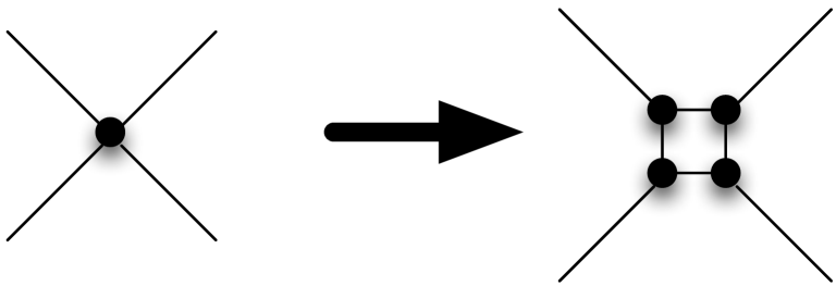
Recall that ${\cal B}^{\div}(P)$ is the brick-contracted graph, in which each brick of ${\cal B}^{+}(P)$ is contracted to a vertex. Recall that a parcel $P$ is a subgraph of $MG$ and defines a set of bricks contained by the faces of $P$ . The planar dual of the parcel has a spanning tree $T$ of depth $\eta+1$ . The algorithm transforms $T$ into a spanning tree $T^{\prime}$ of the planar dual of ${\cal B}^{\div}(P)$ as follows. Each brick is a vertex of $T$ ; replace that vertex with a cycle minus one edge consisting of the duals of the portal edges, as shown in Figure 12.

Since each brick has at most $\theta$ portal edges, it follows that the spanning tree $T^{\prime}$ of the dual of ${\cal B}^{\div}(P)$ has depth at most $(\eta+1)\theta$ . Next, the algorithm defines $\widehat{T}$ to be the set of edges of ${\cal B}^{\div}(P)$ whose duals are not in $T^{\prime}$ . A classical result on planar graphs implies that $\widehat{T}$ is a spanning tree of ${\cal B}^{\div}(P)$ . The construction ensures that each vertex of ${\cal B}^{\div}(P)$ that corresponds to a brick has only one incident edge in $\widehat{T}$ . By our assumption that each vertex in the input graph has degree at most three, every vertex of ${\cal B}^{\div}(P)$ that appears in $G$ has degree at most three in $\widehat{T}$ . Thus $\widehat{T}$ has degree at most three. The bound on the depth of $T^{\prime}$ ensures that, for each vertex $v$ of $\widehat{T}$ , the graph ${\cal B}^{\div}(P)$ contains at most $2(\eta+1)(\theta+1)+1$ edges between descendents of $v$ and non-descendents.

6.3 The dynamic programming table

The algorithm considers the spanning tree $\widehat{T}$ of ${\cal B}^{\div}(P)$ as rooted at an arbitrary leaf. By our assumption that the input graph has degree three, each vertex $v$ of $\widehat{T}$ has at most two children. Let $\widehat{T}(v)$ denote the subtree of $\widehat{T}$ rooted at $v$ . For each vertex $v$ of $\widehat{T}$ , define

f(v)=\left\{\begin{array}[]{ll}B&\mbox{if $v$ is the result of contracting a brick }B\\ v&\mbox{otherwise}\end{array}\right.

and define $W(v)$ to be the subgraph of ${\cal B}^{+}(P)$ induced by $\bigcup\{f(w):w\in\widehat{T}(v)\}$ . Let $\delta(S)$ be the subset of edges with exactly one endpoint in the subgraph $S$ (i.e. a cut). It follows that the cut $\delta(W(v))$ in ${\cal B}^{+}(P)$ is equal to the cut $\delta(\widehat{T}(v))$ in ${\cal B}^{\div}(P)$ and so has $O(\theta\eta)$ edges. The dynamic programming table will be indexed over configurations, defined below.

6.3.1 Configurations

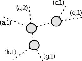
Let $L=\delta(H)$ for a connected, vertex-induced subgraph $H$ of ${\cal B}^{+}(P)$ . We define a configuration $K_{L}$ corresponding to $L$ , illustrated in Figure 13. First, for each edge $e\in L$ , we defined two edges $e^{1}$ and $e^{2}$ to reflect the fact that an edge can be used twice. Let $\hat{L}$ be the resulting set of edges, $\hat{L}=\bigcup_{e\in L}\{e^{1},e^{2}\}$ . A configuration is a forest with no degree-2 vertices whose leaf edges are a subset of $\hat{L}$ , and such that, for each edge $e\in L$ , if the forest contains both $e^{1}$ and $e^{2}$ then these two edges are incident to the same vertex in the forest, together with a $\{1,2\}$ labeling of the internal vertices. We denote the set of all configurations on edge set $L$ by ${\cal K}_{L}$ .

Lemma 6.3.

The number of configurations for $H$ where $n=|\delta(H)|$ is at most $16^{n}(2n)^{2n-2}$ and these trees can be computed in $O(16^{n}(2n)^{2n-2})$ time.

Proof.

A configuration can be selected as follows. First, for each of the $n$ edges, decide whether edge $e^{1}$ is to be included and whether $e^{2}$ is to be included. (There are $4^{n}$ choices.) Let $n^{\prime}$ be the number of edges $e$ for which either $e^{1}$ or $e^{2}$ is to be included. Next, select a tree with the selected edges as leaf edges. It follows from Cayley’s formula that the number of such trees is $2n^{\prime 2n^{\prime}-2}$ , which is at most $2n^{2n-2}$ . Next, delete some subset of non-leaf edges of the tree. There are at most $2^{n}$ ways of selecting such a subset. Finally, select a $\{1,2\}$ labeling of the internal vertices. There are at most $2^{n}$ such labelings.

The set of trees can be computed in $O(1)$ amortized time per tree [22]. ∎

Connecting

A configuration $K_{L}\in{\cal K}_{L}$ is connecting if, for each internal vertex $v$ of $K_{L}$ , if $v$ has label $c$ then $K_{L}$ contains $c$ paths from $v$ to leaves.

Compatibility

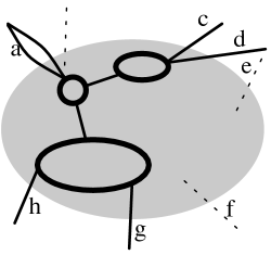
Configurations $K_{A}\in{\cal K}_{A}$ and $K_{B}\in{\cal K}_{B}$ are compatible if for every edge $e\in\hat{A}\cap\hat{B}$ either $e\in K_{A}\cap K_{B}$ or $e\notin K_{A}\cup K_{B}$ .

Compressed bridge-block forest

For a graph $G$ , a block is a maximal subgraph such that, for every two vertices $u$ and $v$ in the subgraph, there are two edge-disjoint $u$ -to- $v$ paths. Contracting each block of $G$ to a single vertex yields the bridge-block forest of $G$ . It is easy to see that it is indeed a forest. An edge $e$ of $G$ is an edge of this forest if $e$ is a bridge of $G$ , i.e. if the endpoints of $e$ are in different connected components of $G-e$ .

We define the compressed bridge-block forest to be the forest obtained from the bridge-block forest by substituting an edge for each maximal path of internal degree two. We denote the compressed bridge-block forest of $G$ by $\widetilde{EC}(G)$ .

Consistency

We say a configuration $K_{A}$ is consistent with a set of mutually compatible configurations $\{K_{A_{1}},K_{A_{2}},\ldots\}$ if

•

there is an isomorphism between $K_{A}$ and $\widetilde{EC}(\cup_{i}K_{A_{i}})$ that preserves the identity of leaf edges of $K_{A}$ , and
•

for each vertex $x$ of $\cup_{i}K_{A_{i}}$ that is labeled 2, $x$ is in a block of $\cup_{i}K_{A_{i}}$ that corresponds to a vertex in $K_{A}$ that is labeled 2.

Meeting

Let $H$ be a connected, vertex-induced subgraph of $G$ . Let $M$ be a minimal solution to an instance $(G,\bm{r})$ . Let $M_{H}$ be the graph obtained from $M$ as follows. Remove edges not in $H\cup\delta(H)$ . Next, for each vertex $v$ outside of $H$ , if $v$ has $k$ incident edges, replace $v$ with $k$ copies of $v$ , one incident to each of these edges.

We say $M$ meets a configuration $K_{\delta(H)}$ if $\widetilde{EC}(M_{H})=K_{\delta(H)}$ and if, for each terminal $x$ in $H$ , $M_{H}$ either contains $r(x)$ edge-disjoint paths to vertices outside of $H$ or contains $\min\{r(x),r(y)\}$ edge-disjoint paths to every other terminal $y$ .

DP table entry

The dynamic program constructs a table $DP_{v}$ for each vertex $v$ of $\widehat{T}$ . The table $DP_{v}$ is indexed by the configurations of $\delta(W(v))$ . We showed in Section 6.1 that we can restrict our attention to solutions with the following property:

the intersection with each brick is a cardinality-at-most- $3\theta$ collection of minimum-cost trees whose leaves are portals.

For each configuration $K$ of $\delta(W(v))$ , the entry $DP_{v}[K]$ is the minimum cost of a subgraph of $W(v)$ that meets configuration $K$ and has the above property. We do not count the cost of edges of $\delta(W(v))$ .

6.3.2 The filling procedure

If $u$ is not a leaf of $\widehat{T}$ , then we populate the entries of $DP_{u}$ with the procedure fill. We use the shorthand $K$ for $K_{\delta(\{u\})}$ and $K_{i}$ for $K_{\delta(W(u_{i}))}$ . The cuts are with respect to the graph ${\cal B}^{+}(P)$ .

fill $(DP_{u})$
	Initialize each entry of $DP_{u}$ to $\infty$ .
	Let $u_{1},\ldots,u_{s}$ be the children of $u$ .
	For every set of connecting, mutually compatible configurations $K,K_{1},\ldots,K_{s}$ ,
		For every connecting configuration $K_{0}$ that is consistent with $K,K_{1},\ldots,K_{s}$ ,
			$\mbox{cost}\leftarrow\bm{c}(K\cap(\cup_{i=1}^{s}K_{i}))+(\bm{c}(K_{1}\cap K_{2})\text{ if }s=2\text{ else }0)+\sum_{i=1}^{s}DP_{u_{i}}[K_{i}]$ .
			$DP_{u}[K_{0}]\leftarrow\min\{DP_{u}[K_{0}],\mbox{cost}\}$

Since $\widehat{T}$ has degree at most three, the number $s$ of children of each vertex $u$ in $\widehat{T}$ is at most two.

If $u$ is a leaf of $\widehat{T}$ and $u$ does not correspond to a brick (i.e. $f(u)=u$ ), the problem is trivial. Each configuration $K$ is a star: $u$ is the center vertex, and the edges of $\delta(\{u\})$ are the edges of $K$ . Since the cost of any subgraph that is induced by $\{u\}$ is zero, the value of $DP_{u}[K]$ is zero for every $K$ .

Suppose $u$ is a leaf of $\widehat{T}$ and $f(u)$ is a brick $B$ . Recall that we restrict our attention to solutions whose intersection with $B$ is a collection of at most $3\theta$ minimum-cost trees whose leaves are portals. The algorithm populates the table $DP_{u}$ as follows. Initialize each entry of $DP_{u}$ to $\infty$ . Next, iterate over cardinality-at-most- $3\theta$ families of subsets of the portals. For each family $\cal F$ ,

•

define a subgraph $H_{\cal F}$ to be the multi-set union over subsets $P$ in $\cal F$ of a minimum-cost tree spanning $P$ ,
•

find the configuration $K$ corresponding to $H_{\cal F}$ , and
•

set $DP_{u}[K]\leftarrow\min\{DP_{u}[K],\text{cost of }H_{\cal F}\}$ .

The minimum-cost tree spanning a subset of portals can be computed in $O(\theta^{3}n)$ time using the algorithm of Theorem 2.1.

6.3.3 Running time

Consider the time required to populate the $DP_{u}$ for all the leaves $u$ of $\widehat{T}$ . We need only consider non-crossing partitions of subsets of $\delta(W(v))$ since $H_{K}$ is the union of non-crossing trees. The number of non-crossing partitions of an $n$ element ordered set is the $n^{th}$ Catalan number, which is at most $4^{n}/(n+1)$ . Therefore, the number of non-crossing sub-partitions is at most $4^{n}$ . It follows that the time to populate $DP_{v}$ for $v$ a brick vertex is $O(\theta^{4}4^{\theta}|B|)$ which is $O(2^{\mathrm{poly}(1/\epsilon)}|B|)$ since $\theta$ depends polynomially on $1/\epsilon$ . Since a vertex appears at most twice in the set of bricks, the time needed to solve all the base cases in $O(2^{\mathrm{poly}(1/\epsilon)}n)$ where $n$ is the number of vertices in the parcel.

Consider the time required to populate the $DP_{u}$ for all the internal vertices $u$ of $\widehat{T}$ . The number of edges in $\delta(W(v))$ in ${\cal B}^{+}(P)$ is $O(\theta\eta)$ . By Lemma 6.3, it follows that the corresponding number of configurations is $O(2^{\mathrm{poly}(1/\epsilon)})$ since $\theta$ and $\eta$ each depend polynomially on $1/\epsilon$ . There are $O(n)$ vertices of the recursion tree and so the time required for the dynamic program, not including the base cases is $O(2^{\mathrm{poly}(1/\epsilon)}n)$ .

The total running time of the dynamic program is $O(2^{\mathrm{poly}(1/\epsilon)}n)$ where $n$ is the number of vertices in the parcel.

6.4 Correctness

The connecting property guarantees that the final solution is feasible (satisfying the conectivity requirements). The definitions of compatible and consistent guarantee the inductive hypothesis.

We show that the procedure fill correctly computes the cost of a minimum-cost subgraph $H_{u}$ of $W(u)$ that meets the configuration $K_{0}$ . We have shown that this is true for the leaves of the recursion tree. Since $K$ is the configuration corresponding to the cut $\delta(\{u_{0}\})$ , $K$ is a star. Therefore $\bm{c}(K)$ is the cost of the edges of $\delta(\{u_{0}\})$ : $K$ is both the configuration and a minimum-cost subgraph that meets that configuration. Further, $\bm{c}(K\cap(\cup_{i=1}^{s}K_{i}))$ is the cost of the edges of $K$ that are in $K_{i}$ (for $i=1,\ldots,s$ ). $w(\cap_{i=1}^{s}K_{i})$ is equal to the cost of the edges common to $K_{1}$ and $K_{2}$ if $s=2$ and zero otherwise. By the inductive hypothesis the cost computed is that of a $H_{u}$ : the subgraph of $W(u)$ of a minimum-cost graph that meets this configuration.

Consider the entries of $DP_{r}$ where $r$ is the root of $\widehat{T}$ . Since $\delta(W(r))$ is empty, there is only one configuration corresponding to this subproblem: the trivial configuration. Therefore, the dynamic program finds the optimal solution in ${\cal B}^{+}(P)$ .

As argued in Section 4.4, combining parcel solutions forms a valid solution in our input graph. We need to compare the cost of the output to the cost of an optimal solution.

Recall that new terminals are added at the parcel boundaries to guarantee connectivity between the parcels; let $\bm{r}^{+}$ denote the requirements including these new terminals. Let $S(G,\bm{r})$ denote the optimal solution in graph $G$ with requirements $\bm{r}$ .

For each parcel $P$ , there is a (possibly empty) solution $S_{P}$ in ${\cal B}^{+}(P)$ for the original and new terminals in $P$ consisting of edges of $S({\cal B}^{+}(\text{\it MG}),\bm{r})\cup\partial{\cal H}$ (where $\cal H$ is the set of parcels and $\partial{\cal H}$ is the set of boundary edges of all parcels). We have:

\bm{c}(S({\cal B}^{+}(\text{\it MG}),\bm{r})\cap{\cal B}^{+}(P))\leq\bm{c}(S_{P})=\bm{c}(S_{P}-\partial{\cal H})+\bm{c}(S_{P}\cap\partial{\cal H}).

Every edge of $S({\cal B}^{+}(\text{\it MG}),\bm{r})$ not in $\partial{\cal H}$ appears in $S_{P}$ for exactly one parcel $P$ , and so

\sum_{P\in{\cal H}}\bm{c}(S_{P}-\partial{\cal H})\leq\bm{c}(S({\cal B}^{+}(\text{\it MG}),\bm{r})).

Every edge of $\partial{\cal H}$ appears in at most two parcels, and so

\sum_{P\in{\cal H}}\bm{c}(S_{P}\cap\partial{\cal H})\leq 2\cdot\bm{c}(\partial{\cal H}).

Since a feasible solution for the original and new terminals in ${\cal B}^{+}(\text{\it MG})$ can be obtained by adding a subset of the edges of $\partial{\cal H}$ to $S({\cal B}^{+}(\text{\it MG}),\bm{r})$ , the cost of the output of our algorithms is at most

\bm{c}(\partial{\cal H})+\sum_{P\in{\cal H}}{S({\cal B}^{+}(P),\bm{r}^{+})}\leq\bm{c}(S({\cal B}^{+}(\text{\it MG}),\bm{r}))+3\bm{c}(\partial{\cal H}).

Combining the cost of the parcel boundaries, the definition of $\eta$ , and the cost of the mortar graph, we obtain $\bm{c}(\partial{\cal H})\leq\frac{1}{2}\epsilon\bm{c}(S(G,\bm{r}))=\frac{1}{2}\epsilon{\rm OPT}$ . Finally, by Theorem 4.6, the cost of the output is at most $(1+c\epsilon)\ {\rm OPT}$ . This gives:

Theorem 6.4.

There is an approximation scheme for solving the $\{0,1,2\}$ -edge connectivity problem (allowing duplication of edges) in planar graphs. The running time is $O(2^{\mathrm{poly}(1/\epsilon)}n+n\log n)$ .

Comments

The PTAS framework used is potentially applicable to problems where (i) the input consists of a planar graph $G$ with edge-costs and a subset $Q$ of the vertices of $G$ (we call $Q$ the set of terminals), and where (ii) the output spans the terminals. Steiner tree and two-edge-connectivity have been solved using this framework. The PTAS for the subset tour problem [18] (which was the inspiration for this framework) can be reframed using this technique. Since the extended abstract of this work first appeared, Borradaile, Demaine and Tazari have also this framework to give PTASes for the same set of problems in graphs of bounded genus [6], Bateni, Hajiaghayi and Marx [3] have extended the framework to the Steiner forest problem and Bateni et al. [2] have extended the framework to prize collecting problems.

Acknowledgements

The authors thank David Pritchard for comments on early versions of this work and discussions with Baigong Zheng regarding Theorems 2.5 and 2.6. This material is based upon work supported by the National Science Foundation under Grant Nos. CCF-0964037, CCF-0963921, CCF-14-09520 and by a Natural Science and Research Council of Canada Postdoctoral Fellowship.

References

[1] B. Baker. Approximation algorithms for NP-complete problems on planar graphs. Journal of the ACM, 41(1):153–180, 1994.
[2] M. Bateni, C. Chekuri, A. Ene, M. Hajiaghayi, N. Korula, and D. Marx. Prize-collecting Steiner problems on planar graphs. In Proceedings of the 22nd Annual ACM-SIAM Symposium on Discrete Algorithms, pages 1028–1049, 2011.
[3] M. Bateni, M. Hajiaghayi, and D. Marx. Approximation schemes for Steiner forest on planar graphs and graphs of bounded treewidth. J. ACM, 58(5):21, 2011.
[4] A. Berger, A. Czumaj, M. Grigni, and H. Zhao. Approximation schemes for minimum 2-connected spanning subgraphs in weighted planar graphs. In Proceedings of the 13th European Symposium on Algorithms, volume 3669 of Lecture Notes in Computer Science, pages 472–483, 2005.
[5] A. Berger and M. Grigni. Minimum weight 2-edge-connected spanning subgraphs in planar graphs. In Proceedings of the 34th International Colloquium on Automata, Languages and Programming, volume 4596 of Lecture Notes in Computer Science, pages 90–101, 2007.
[6] G. Borradaile, E. Demaine, and S. Tazari. Polynomial-time approximation schemes for subset-connectivity problems in bounded-genus graphs. Algorithmica, 2012. Online.
[7] G. Borradaile, C. Kenyon-Mathieu, and P. Klein. A polynomial-time approximation scheme for Steiner tree in planar graphs. In Proceedings of the 18th Annual ACM-SIAM Symposium on Discrete Algorithms, pages 1285–1294, 2007.
[8] G. Borradaile, P. Klein, and C. Mathieu. Steiner tree in planar graphs: An ${O}(n\log n)$ approximation scheme with singly exponential dependence on epsilon. In Proceedings of the 10th International Workshop on Algorithms and Data Structures, volume 4619 of Lecture Notes in Computer Science, pages 275–286, 2007.
[9] G. Borradaile, P. Klein, and C. Mathieu. An ${O}(n\log n)$ approximation scheme for Steiner tree in planar graphs. ACM Transactions on Algorithms, 5(3):1–31, 2009.
[10] A. Czumaj and A. Lingas. On approximability of the minimum cost k-connected spanning subgraph problem. In Proceedings of the 10th Annual ACM-SIAM Symposium on Discrete Algorithms, pages 281–290, 1999.
[11] R. Erickson, C. Monma, and A. Veinott. Send-and-split method for minimum-concave-cost network flows. Mathematics of Operations Research, 12:634–664, 1987.
[12] K. Eswaran and R. Tarjan. Augmentation problems. SIAM Journal on Computing, 5(4):653–665, 1976.
[13] G. Frederickson and J. Jájá. Approximation algorithms for several graph augmentation problems. SIAM Journal on Computing, 10(2):270–283, 1981.
[14] M. Goemans, A. Goldberg, S. Plotkin, D. Shmoys, É. Tardos, and D. Williamson. Improved approximation algorithms for network design problems. In Proceedings of the 5th Annual ACM-SIAM Symposium on Discrete Algorithms, pages 223–232, 1994.
[15] M. Henzinger, P. Klein, S. Rao, and S. Subramanian. Faster shortest-path algorithms for planar graphs. Journal of Computer and System Sciences, 55(1):3–23, 1997.
[16] K. Jain. A factor 2 approximation algorithm for the generalized Steiner network problem. Combinatorica, 2001(1):39–60, 21.
[17] S. Khuller and U. Vishkin. Biconnectivity approximations and graph carvings. Journal of the ACM, 41(2):214–235, 1994.
[18] P. Klein. A subset spanner for planar graphs, with application to subset TSP. In Proceedings of the 38th Annual ACM Symposium on Theory of Computing, pages 749–756, 2006.
[19] P. Klein. A linear-time approximation scheme for TSP in undirected planar graphs with edge-weights. SIAM Journal on Computing, 37(6):1926–1952, 2008.
[20] P. Klein and R. Ravi. When cycles collapse: A general approximation technique for constraind two-connectivity problems. In Proceedings of the 3rd International Conference on Integer Programming and Combinatorial Optimization, pages 39–55, 1993.
[21] K. Mehlhorn. A faster approximation algorithm for the Steiner problem in graphs. Information Processing Letters, 27(3):125–128, 1988.
[22] S. Nakano and T. Uno. Efficient generation of rooted trees. Technical Report NII-2003-005E, National Institute of Informatics, 2003.
[23] R. Ravi. Approximation algorithms for Steiner augmentations for two-connectivity. Technical Report TR-CS-92-21, Brown University, 1992.
[24] M. Resende and P. Pardalos, editors. Handbook of Optimization in Telecommunications. Springer, 2006.
[25] H. Whitney. Non-separable and planar graphs. Trans. Amer. Math. Soc., 34:339–362, 1932.
[26] P. Widmayer. A fast approximation algorithm for Steiner’s problem in graphs. In Graph-Theoretic Concepts in Computer Science, volume 246 of Lecture Notes in Computer Science, pages 17–28. Springer Verlag, 1986.
[27] D. Williamson, M. Goemans, M. Mihail, and V. Vazirani. A primal-dual approximation algorithm for generalized Steiner network problems. In Proceedings of the 25th Annual ACM Symposium on Theory of Computing, pages 708–717, 1993.
[28] Y. Wu, P. Widmayer, and C. Wong. A faster approximation algorithm for the Steiner problem in graphs. Acta informatica, 23(2):223–229, 1986.

The two-edge connectivity survivable-network design problem in planar graphs

Abstract

1 Introduction

Two edge-connected spanning subgraphs

Beyond spanning

1.1 Summary of new results

Theorem 1.1.

Theorem 1.2.

1.2 Organization

2 Basics

Theorem 2.1.

2.1 Edge-connectivity basics

Lemma 2.2 (Transitivity).

Lemma 2.3 (Empty Cycle).

Proof.

2.2 Vertex-connectivity basics

Lemma 2.4.

Proof.

Theorem 2.5.

Proof.

Theorem 2.6.

Proof.

3 An exact algorithm for boundary {0,1,2}\{0,1,2\}-edge connectivity

Corollary 3.1.

Lemma 3.2.

Proof.

Lemma 3.3.

Proof.

Lemma 3.4.

Proof.

4 A PTAS framework for connectivity problems in planar graphs

4.1 Mortar graph and bricks

Definition 4.1.

Lemma 4.2 (Lemma 6.10 [9]).

Lemma 4.3 (Lemma 6.6 [9]).

4.2 Portals and simple connections

Lemma 4.4 (Lemma 7.1 [9]).

Lemma 4.5.

4.3 Structure Theorem

Theorem 4.6 (Structure Theorem).

4.4 Approximation scheme

5 Proof of the Structure Theorem

Definition 5.1 (Joining vertex).

Lemma 5.2 (Simplifying a tree with one root, Lemma 10.4 [9]).

Lemma 5.3 (Simplifying a tree with two roots, Lemma 10.6 [9]).

Lemma 5.4.

Proof.

5.1 Construction of a new solution

5.1.1 Augment

Lemma 5.5.

5.1.2 Cleave

Lemma 5.6.

Proof.

Corollary 5.7.

Lemma 5.8.

Lemma 5.9.

Lemma 5.10.

Proof.

Lemma 5.11.

Proof.

5.1.3 Flatten

5.1.4 Map

5.1.5 Restructure

Connected case:

Disconnected case:

Number of joining vertices

5.1.6 Rejoin

5.2 Analysis of connectivity

5.3 Analysis of cost increase

6 Dynamic Program

6.1 Structure of solution

Lemma 6.1.

Proof.

Corollary 6.2.

Proof.

6.2 The tree used to guide the dynamic program

6.3 The dynamic programming table

6.3.1 Configurations

Lemma 6.3.

Proof.

3 An exact algorithm for boundary $\{0,1,2\}$ -edge connectivity