The Unbounded Denominators Conjecture

Frank Calegari fcale@math.uchicago.edu The University of Chicago, 5734 S University Ave, Chicago, IL 60637, USA , Vesselin Dimitrov vesselin.dimitrov@gmail.com Department of Mathematics, California Institute of Technology, Pasadena, CA 91125, USA and Yunqing Tang yungqing.tang@berkeley.edu Department of Mathematics, University of California, Berkeley, Evans Hall, Berkeley, CA 94720, USA

Abstract.

We prove the unbounded denominators conjecture in the theory of noncongruence modular forms for finite index subgroups of $\mathrm{SL}_{2}(\mathbf{Z})$ . Our result includes also Mason’s generalization of the original conjecture to the setting of vector-valued modular forms, thereby supplying a new path to the congruence property in rational conformal field theory. The proof involves a new arithmetic holonomicity bound of a potential-theoretic flavor, together with Nevanlinna second main theorem, the congruence subgroup property of $\mathrm{SL}_{2}(\mathbf{Z}[1/p])$ , and a close description of the Fuchsian uniformization $D(0,1)/\Gamma_{N}$ of the Riemann surface $\mathbf{C}\smallsetminus\mu_{N}$ .

F.C. was supported in part by NSF Grant DMS-2001097. Y.T. was supported in part by NSF grant DMS-2231958 and a Sloan Research Fellowship. Some of the work was done when Y.T. was at CNRS and Université Paris-Saclay from February 2020 to June 2021 and at Princeton University from July 2021 to June 2022.

1. Introduction

We prove the following:

Theorem 1.0.1 (Unbounded Denominators Conjecture).

Let $N$ be any positive integer, and let $f(\tau)\in\mathbf{Z}\llbracket q^{1/N}\rrbracket$ for $q=\exp(\pi i\tau)$ be a holomorphic function on the upper half plane $\mathbf{H}$ . Suppose there exists an integer $k$ and a finite index subgroup $\Gamma\subset\mathrm{SL}_{2}(\mathbf{Z})$ such that

f\left(\frac{a\tau+b}{c\tau+d}\right)=(c\tau+d)^{k}f(\tau),\quad\quad\textrm{for all }\left(\begin{matrix}a&b\\ c&d\end{matrix}\right)\in\Gamma,

and suppose that $f(\tau)$ is meromorphic at the cusps, that is, locally extends to a meromorphic function near every cusp in the compactification of $\mathbf{H}/\Gamma$ . Then $f(\tau)$ is a modular form for a congruence subgroup of $\mathrm{SL}_{2}(\mathbf{Z})$ .

The contrapositive of this statement is equivalent to the following, which explains the name of the conjecture: if $f(\tau)\in\mathbf{Q}\llbracket q^{1/N}\rrbracket$ is a modular form which is not modular for some congruence subgroup, then the coefficients of $f(\tau)$ have unbounded denominators. The corresponding statement remains true if one replaces $\mathbf{Q}$ by any number field (see Remark 6.3.1).

Let $\lambda(\tau)$ be the modular lambda function (Legendre’s parameter):

(1.0.2)

\frac{\lambda(\tau)}{16}=\left(\frac{\eta(\tau/2)\eta(2\tau)^{2}}{\eta(\tau)^{3}}\right)^{8}=q\prod_{n=1}^{\infty}\left(\frac{1+q^{2n}}{1+q^{2n-1}}\right)^{8}=q-8q^{2}+\cdots

with $q=e^{\pi i\tau}$ and $\eta(\tau/2)=q^{1/24}\prod_{n=1}^{\infty}(1-q^{n})$ . (Historic conventions force one to use $q$ for both $e^{\pi i\tau}$ and $e^{2\pi i\tau}$ — we use the first choice unless we expressly state otherwise.) On replacing the weight $k$ form $f$ by the weight zero form $f(\tau)(\lambda(\tau)/16\eta(\tau/2)^{2})^{k}$ , we may (and do) assume that $k=0$ . The function $f$ is then an algebraic function of $\lambda$ , with branching only at the three punctures $\lambda=0,1,\infty$ of the modular curve $Y(2)\cong\mathbf{P}^{1}\smallsetminus\{0,1,\infty\}$ . Thus another reading of our result states that the Belyĭ maps (étale coverings)

\pi:U\to\mathbf{CP}^{1}\smallsetminus\{0,1,\infty\}:=\mathrm{Spec}\,\mathbf{C}[\lambda,1/\lambda,1/(1-\lambda)]=Y(2)

possessing a formal Puiseux branch in $\mathbf{Z}\llbracket\lambda(\tau/m)/16\rrbracket\otimes\mathbf{C}$ for some $m\in\mathbf{N}_{>0}$ are exactly the congruence coverings $Y_{\Gamma}=\mathbf{H}/\Gamma\to\mathbf{H}/\Gamma(2)=Y(2)$ , with $\Gamma$ ranging over all congruence subgroups of $\Gamma(2)$ . The reverse implication is a theorem of Shimura [Shi59] (presented in his book as [Shi71, Theorem 3.52]), and reflects the fact that the $q$ -expansions of eigenforms on congruence subgroups are determined by their Hecke eigenvalues (see also [Kat73, § 1.2]).

We refer the reader to Atkin and Swinnerton-Dyer [ASD71] for the roots of the unbounded denominators conjecture, and to Birch’s article [Bir94] as well as to Long’s survey [Lon08, § 5] for an introduction to this problem and its history. For the vector-valued generalization, see § 7.3 and its references below. The cases of relevance to the partition and correlation functions of rational conformal field theories (of which the tip of the iceberg is the example (1.0.3) discussed below) were resolved in a string of works [DR18, DLN15, SZ12, NS10, Xu06, Ban03, Zhu96, AM88], by the modular tensor categories method. Some further sporadic cases of the unbounded denominators conjecture have been settled by mostly ad hoc means [FF22, FM16b, LL12, KL08, KL09].

To give some simple examples, the integrality property $\sqrt[8]{1-x}\in\mathbf{Z}\llbracket x/16\rrbracket$ corresponds to the fact that the modular form $(\lambda/16)^{1/8}=q^{1/8}\prod_{n=1}^{\infty}(1+q^{2n})(1+q^{2n-1})^{-1}$ and the affine Fermat curve $x^{8}+y^{8}=1$ are congruence; whereas a simple non-example [Lon08, § 5.5] is the affine Fermat curve $x^{n}+y^{n}=1$ for $n\notin\{1,2,4,8\}$ , for which the fact that its Fuchsian group is a noncongruence arithmetic group is detected arithmetically by the calculation $\sqrt[n]{1-x}\notin\mathbf{Z}\llbracket x/16\rrbracket\otimes\mathbf{C}$ . This recovers a classical theorem of Klein [KF17, page 534]. To include an example related to two-dimensional rational conformal field theories, consider the following function (with $q=e^{2\pi i\tau}$ ):

(1.0.3)

j(\tau)^{1/3}=q^{-1/3}\,\frac{1+240\sum_{n=1}^{\infty}\sigma_{3}(n)q^{n}}{\prod_{n=1}^{\infty}(1-q^{n})^{8}}=q^{-1/3}(1+248q+4124q^{2}+34752q^{3}+\cdots).

The resulting Fourier coefficients are closely linked to the dimensions of the irreducible representations of the exceptional Lie group $E_{8}(\mathbf{C})$ , and in particular they are integers. To be more precise: the modular function $j^{1/3}$ coincides with the graded dimension of the level one highest-weight representation of the affine Kac–Moody algebra $E_{8}^{(1)}$ ; see Gannon’s book [Gan06, § 0.5 and § 3.2.3] for a broad view on this topic and its relation to mathematical physics. The unbounded denominators conjecture (Theorem 1.0.1) now implies that $j^{1/3}$ must be a modular function on a congruence subgroup. (Strictly speaking, since $j^{1/3}$ is a Laurent series rather than a power series, one applies Theorem 1.0.1 to $j^{1/3}\cdot\Delta$ and then divides through by $\Delta$ .) One readily confirms that $j^{1/3}$ is a Hauptmodul for the level $3$ subgroup which is the kernel of the composite $\mathrm{PSL}_{2}(\mathbf{Z})\rightarrow\mathrm{PSL}_{2}(\mathbf{F}_{3})=A_{4}\rightarrow\mathbf{Z}/3\mathbf{Z}$ . One final example is the function

(1.0.4)

h:=\frac{\lambda(\tau)(1-\lambda(\tau))}{16}=\left(\frac{\eta(\tau/2)\eta(2\tau)}{\eta(\tau)^{2}}\right)^{24}

of level $\Gamma^{0}(2)\supset\Gamma(2)$ ; here the complete list of $n$ for which $h^{1/n}$ is either congruence modular or has bounded denominators are the divisors of $24$ . The claim that $h^{1/n}$ has bounded denominators for $n|24$ is apparent from the product formula in Equation 1.0.4, and the claim that $h^{1/n}$ does not have bounded denominators for $n\nmid 24$ is an elementary exercise. We can directly compute when is $h^{1/n}$ congruence, as follows. By Kummer theory, the extension $\mathbf{C}(h^{1/n})$ of the function field $\mathbf{C}(h)$ of $\mathbf{H}/\Gamma^{0}(2)$ is Galois with Galois group $\mathbf{Z}/n\mathbf{Z}$ . Since $h$ is nonvanishing on $\mathbf{H}$ , this extension is unramified away from the cusps, and so gives rise to a homomorphism $\Gamma^{0}(2)\rightarrow\mathbf{Z}/n\mathbf{Z}$ ; the function $h^{1/n}$ is modular for the kernel $\Gamma$ of this homomorphism. Now $h^{1/n}$ is congruence if and only if the latter map factors through the congruence completion $\widehat{\Gamma^{0}(2)}$ of $\Gamma^{0}(2)$ ; here, $\Gamma^{0}(2)$ is considered as a subgroup of $\mathrm{PSL}_{2}(\mathbf{Z})$ . In fact, one may compute that the abelianization of $\Gamma^{0}(2)$ is $\mathbf{Z}\oplus\mathbf{Z}/2\mathbf{Z}$ whereas the abelianization of $\widehat{\Gamma^{0}(2)}$ is $\mathbf{Z}/24\mathbf{Z}\oplus\mathbf{Z}/2\mathbf{Z}$ . The other $\mathbf{Z}/2\mathbf{Z}$ extension corresponds to the congruence modular form $\sqrt{1-64h}=1-2\lambda$ .

In a similar vein pertaining to the examples from the representation theory of vertex operator algebras, we prove in our closing § 7 the natural generalization of Theorem 1.0.1 to components of vector-valued modular forms for $\mathrm{SL}_{2}(\mathbf{Z})$ , in particular resolving — in a sharper form, in fact — Mason’s unbounded denominators conjecture [Mas12, KM08] on generalized modular forms.

1.1. A sketch of the main ideas

Our proof of Theorem 1.0.1 follows a broad Diophantine analysis path known in the literature (see [Bos04, Bos13] or [Bos20, Chapter 10]) as the arithmetic algebraization method.

1.1.1. The Diophantine principle

The most basic antecedent of these ideas is the following easy lemma:

Lemma 1.1.2.

A power series $f(x)=\sum_{n=0}^{\infty}a_{n}x^{n}\in\mathbf{Z}\llbracket x\rrbracket$ which defines a holomorphic function on $D(0,R)$ for some $R>1$ is a polynomial.

Lemma 1.1.2 follows upon combining the following two observations, fixing some $1>\eta>R^{-1}$ :

(1)

The coefficients $a_{n}$ are either $0$ or else $\geq 1$ in magnitude.
(2)

The Cauchy integral formula gives a uniform upper bound $|a_{n}|=o(\eta^{n})$ .

We shall refer to the first inequality as a Liouville lower bound, following its use by Liouville in his proof of the lower bound $|\alpha-p/q|\gg 1/q^{n}$ for algebraic numbers $\alpha\neq p/q$ of degree $n\geq 1$ . We shall refer to the second inequality as a Cauchy upper bound, following the example above where it comes from an application of the Cauchy integral formula. The first nontrivial generalization of Lemma 1.1.2 was Émile Borel’s theorem [Bor94]. Dwork famously used a $p$ -adic generalization of Borel’s theorem in his $p$ -adic analytic proof of the rationality of the zeta function of an algebraic variety over a finite field (see Dwork’s account in the book [DGS94, Chapter 2]). The simplest nontrivial statement of Borel’s theorem is that an integral formal power series $f(x)\in\mathbf{Z}\llbracket x\rrbracket$ must already be a rational function as soon as it has a meromorphic representation as a quotient of two convergent complex-coefficients power series on some disc $D(0,R)$ of a radius $R>1$ . The subject of arithmetic algebraization blossomed at the hands of many authors, including most prominently Carlson, Pólya, Robinson, Salem, Cantor, D. $\&$ G. Chudnovsky, Bertrandias, Zaharjuta, André, Bost, Chambert-Loir [CL02, BCL09, Ami75], [And04, § I.5], [And89, § VIII]. A simple milestone that we further develop in our § 2 is André’s algebraicity criterion [And04, Théorème 5.4.3], stating in a particular case that an integral formal power series $f(x)\in\mathbf{Z}\llbracket x\rrbracket$ is algebraic as soon as the two formal functions $x$ and $f$ admit a simultaneous analytic uniformization — that means an analytic map $\varphi:(D(0,1),0)\to(\mathbf{C},0)$ such that the composition $f(\varphi(z))\in\mathbf{C}\llbracket z\rrbracket$ of holomorphic function germs also converges on the full disc $D(0,1)$ , and such that $\varphi$ is sufficiently large in terms of conformal size, namely: $|\varphi^{\prime}(0)|>1$ . For example, for any integer $m$ , the algebraic power series $f=(1-m^{2}x)^{1/m}\in\mathbf{Z}\llbracket x\rrbracket$ admits the simultaneous analytic uniformization $x=\varphi(z)=(1-e^{Mz})m^{-2}$ and $f=f(\varphi(z))=e^{Mz/m}$ , where the conformal size $|\varphi^{\prime}(0)|=M/m^{2}$ can clearly be made arbitrarily large by making a suitable choice of $M$ .

A common theme of all these generalizations of Lemma 1.1.2 is that they come down to a tension between a Liouville lower bound and a Cauchy upper bound. For example, in the proof of Borel’s theorem ([Ami75, Ch 5.3]), the Liouville lower bound is applied not to the coefficients $a_{n}$ themselves but rather to Hankel determinants $\det|\alpha_{i,j}|$ with $\alpha_{i,j}=a_{i+j+n}$ . To consider a more complicated example (much closer in both spirit and in details to our own analysis), to prove André’s algebraicity criterion [And04, Théorème 5.4.3], one wants to prove that certain powers of a formal function $f(\mathbf{x})\in\mathbf{Z}\llbracket\mathbf{x}\rrbracket$ are linearly dependent over the polynomial ring $\mathbf{Z}[\mathbf{x}]$ . (It will be advantageous to consider functions in several complex variables $\mathbf{x}=(x_{1},\ldots,x_{d})$ .) The idea is now to consider a certain $\mathbf{Z}[\mathbf{x}]$ linear combination $F(\mathbf{x})$ of powers of $f(\mathbf{x})$ chosen such that they vanish to high order at $\mathbf{0}$ but yet the $\mathbf{Z}[\mathbf{x}]$ coefficients $p(\mathbf{x})$ are themselves not too complicated — the existence of such a choice follows from the classical Siegel’s lemma. Now the Liouville lower bound is applied to a lowest order non-zero coefficient of $F(\mathbf{x})\in\mathbf{Z}\llbracket\mathbf{x}\rrbracket$ . Note that such a coefficient must exist or else the equality $F(\mathbf{x})=0$ realizes $f(\mathbf{x})$ as algebraic. The Cauchy upper bound in this case once again follows by an application of the Cauchy integral formula.

In our setting, the Liouville lower bound ultimately comes down to the integrality (“bounded denominators”) hypothesis on the Fourier coefficients of $f(\tau)$ , while the Cauchy upper bound comes down to studying the mean growth behavior $m(r,\varphi):=\int_{|z|=r}\log^{+}{|\varphi|}\,\mu_{\mathrm{Haar}}$ of the largest (universal covering) analytic map $\varphi:D(0,1)\to\mathbf{C}\smallsetminus\mu_{N}$ avoiding the $N$ -th roots of unity. These are clearly distinguished in our abstract arithmetic algebraization work of § 2 as the steps (2.2.2) and (2.2.3), respectively. (We also refer to (2.4.10) and (2.4.8), resp. (2.5.26) and (2.5.24), in our alternative treatments.) Our Theorem 2.0.1 is effectively a quantitative refinement of André’s algebraicity criterion to take into account the degree of algebraicity over $\mathbf{Q}(x)$ , and still more precisely a certain holonomy rank over $\mathbf{Q}(x)$ . Foreshadowing a key technical point (to be discussed in more detail later in the introduction), our Cauchy upper bound is given in terms of a mean (integrated) growth term rather than a supremum term, and this improvement is essential to our approach.

1.1.3. Modularity and simultaneous uniformizations of $f$ and $\lambda$

Let us now explain the relevance of arithmetic holonomy rank bounds to the unbounded denominators conjecture. After reducing to weight $k=0$ as above, the functions $f=f(\tau)$ and $x:=\lambda(\tau)/16\in q+q^{2}\mathbf{Z}\llbracket q\rrbracket$ are algebraically dependent and share both (we assume) the property of integral Fourier coefficients at the cusp $q=0$ . Let us assume for the purpose of this sketch that $f(\tau)\in\mathbf{Z}\llbracket q\rrbracket$ with $q=e^{\pi i\tau}$ , i.e. that the cusp $i\infty$ has width dividing $2$ . Then the formal inverse series expansion

q=x+8x^{2}+84x^{3}+992x^{4}+\cdots\in x+x^{2}\mathbf{Z}\llbracket x\rrbracket

of (1.0.2) has integer coefficients, expressing the identity $\mathbf{Z}\llbracket q\rrbracket=\mathbf{Z}\llbracket x\rrbracket$ of formal power series rings, and that formal substitution turns our integral Fourier coefficients hypothesis into an algebraic power series with integer coefficients: henceforth in this introductory sketch we switch to writing, by a mild and harmless notational abuse, simply $f(x)\in\mathbf{Z}\llbracket x\rrbracket$ in place of $f(\tau)$ and $\lambda(q)$ in place of $\lambda(\tau)$ . In the general case of arbitrary cusp width, which we need anyhow for the inner workings of our proof even if one is ultimately interested in the $\mathbf{Z}\llbracket q\rrbracket$ case, we will only have $f\in\mathbf{Z}[1/N]\llbracket x\rrbracket$ when we write out $f(\tau)$ as a power series in $x:=\sqrt[N]{\lambda/16}$ to accommodate the Puiseux series — but there is still a hidden integrality property which we can exploit. That leads to some mild technical nuance with the power series (2.0.2) — think of $t=q^{1/N}$ , $x(t)=\sqrt[N]{\lambda(t^{N})/16}$ and $p(x)=x^{N}$ — in our refinement (2.0.3) of André’s theorem.

The complex analysis enters by way of a linear ODE in the following way. To start with, we have, just by fiat, the simultaneous analytic uniformization of the two functions $x:=\lambda/16$ and $f$ by the complex unit $q$ -disc $|q|<1$ . In this way, the tautological choice $\varphi(z):=\lambda(z)/16$ turns our algebraic power series $f(x)\in\mathbf{Z}\llbracket x\rrbracket$ into a boundary case (unit conformal size $\varphi^{\prime}(0)=1$ ) of André’s criterion. Another boundary case, but this time transcendental and incidentally demonstrating the sharpness of the qualitative André algebraicity criterion even in the a priori holonomic situation (see [And04, Appendix, A.5] for a discussion), is provided by the Gauss hypergeometric function

(1.1.4)

F(x):={}_{2}F_{1}{\left[\genfrac{.}{.}{0.0pt}{}{1/2\mskip 8.0mu1/2}{1};16x\right]}=\sum_{n=0}^{\infty}\binom{2n}{n}^{2}x^{n}\in\mathbf{Z}\llbracket x\rrbracket,

whose unit-radius simultaneous analytic uniformization with $x=\lambda/16$ is given again by the analytic $q$ coordinate, and the classical Jacobi formula

(1.1.5)

F(\tau)={}_{2}F_{1}{\left[\genfrac{.}{.}{0.0pt}{}{1/2\mskip 8.0mu1/2}{1};\lambda(q)\right]}=\Big{(}\sum_{n\in\mathbf{Z}}q^{n^{2}}\Big{)}^{2}

which transforms this hypergeometric series into a weight one modular form for the congruence group $\Gamma(2)$ . The existence of such transcendental $\mathbf{Z}\llbracket x\rrbracket$ holonomic functions on $\mathbf{C}\smallsetminus\{0,1/16\}$ recovers—by André’s algebraicity criterion—a classical “ $1/16$ theorem” of Carathéodory [Car54, (412.8) on page 198]. (See also Goluzin [Gol69, § III.1, Theorem 1].)

1.1.6. A finite local monodromy leads to an overconvergence

It turns out, and this is the key to our method and already answers André’s question in [And04, Appendix, A.5], that a different choice of $\varphi(z)$ allows one to arithmetically distinguish between these two cases (algebraic and transcendental), and to have the algebraicity of $f(x)$ recognized by André’s Diophantine criterion by way of an “overconvergence.” Suppose that $f(\tau)$ is a holomorphic modular function and $F(\tau)$ is a holomorphic modular form — concretely, let us take $F(\tau)$ to be the theta series of equation (1.1.5), — and let $f(x)$ and $F(x)$ respectively denote these functions as functions of $x=\lambda/16$ , so $F(x)$ is given by equation (1.1.4). The common feature of these two functions $f(x)$ and $F(x)$ — coming respectively out of modular forms of weights $0$ and $1$ — is that they both vary holonomically in $x\in\mathbf{C}\smallsetminus\{0,1/16\}$ : they satisfy linear ODEs with coefficients in $\mathbf{Q}[x]$ and no singularities¹¹1With nontrivial local monodromy. The precise definition is in 2.0.4. apart from the three punctures $x=0,1/16,\infty$ of $Y(2)=\mathbf{H}/\Gamma(2)$ . The difference feature is that their respective local monodromies around $x=0$ are finite for the case of $f(x)$ (a quotient of $\mathbf{Z}/N$ , with the order $N$ equal to the lowest common multiple of the cusp widths, or Wohlfahrt level [Woh64] of $f(x)$ ); and infinite for the case of $F(x)$ (isomorphic to $\mathbf{Z}$ , corresponding more particularly to the fact that this particular hypergeometric function acquires a $\log{x}$ term after an analytic continuation around a small circle enclosing $x=1/16$ ). If now we perform the variable change $x\mapsto x^{N}$ , redefaulting to $x:=\sqrt[N]{\lambda(q^{N})/16}$ , that resolves the $N$ -th root ambiguity in the formal Puiseux branches of $f(x)$ at $x=0$ , and the resulting algebraic power series $f(x^{N})\in\mathbf{Z}\llbracket x^{N}\rrbracket\subset\mathbf{Z}\llbracket x\rrbracket$ has turned holonomic on $\mathbf{P}^{1}\smallsetminus\{16^{-1/N}\mu_{N},\infty\}$ : singularities only at $16^{-1/N}\mu_{N}\cup\{\infty\}$ (but not at $x=0$ : this key step of exploiting arithmetic algebraization is the same as in Ihara’s arithmetic connectedness theorem [Iha94, Theorem 1], which together with Bost’s extension [Bos99] to arithmetic Lefschetz theorems have in equal measure been inspirational for our whole approach to the unbounded denominators conjecture). Since $\lambda:D(0,1)\to\mathbf{C}\smallsetminus\{1\}$ has fiber $\lambda^{-1}(0)=\{0\}$ , the function $\varphi(z):=\sqrt[N]{\lambda(z^{N})/16}:D(0,1)\to\mathbf{C}\smallsetminus 16^{-1/N}\mu_{N}$ is still holomorphic on the unit disc $|z|<1$ , and under this tautological choice, both functions $f(x^{N})$ and $F(x^{N})$ continue to be at the borderline of André’s algebraicity criterion: $|\varphi^{\prime}(0)|=1$ .

But if instead of the tautological simultaneous uniformization we take

\varphi:D(0,1)\to\mathbf{C}\smallsetminus 16^{-1/N}\mu_{N}

to be the universal covering map (pointed at $\varphi(0)=0$ ), then either by a direct computation with monodromy, or by Cauchy’s analyticity theorem on the solutions of linear ODEs with analytic coefficients and no singularities in a disc, we have both function germs $x:=\varphi(z)$ and $f(x):=f(\varphi(z))$ holomorphic, hence convergent, on the full unit disc $D(0,1)$ . In contrast, now $F(\varphi(z))$ converges only up to the “first” nonzero fiber point in $\varphi^{-1}(0)\smallsetminus\{0\}$ , giving a certain radius rather smaller than $1$ . We must have the strict lower bound $|\varphi^{\prime}(0)|>1$ , because the preceding unit-radius holomorphic map $\sqrt[N]{\lambda(z^{N})/16}:D(0,1)\to\mathbf{C}\smallsetminus 16^{-1/N}\mu_{N}$ has to factorize properly through the universal covering map. Indeed in Theorem 5.1.4, using an explicit description by hypergeometric functions of the multivalued inverse of the universal covering map of $\mathbf{C}\smallsetminus\mu_{N}$ based on Poincaré’s ODE approach [Hem88] to the uniformization of Riemann surfaces, we find an exact formula for this uniformization radius in terms of the Euler Gamma function.²²2André pointed out to us that this explicit formula has previously been obtained by Kraus and Roth, see [KR16, Remark 5.1]. See also [Gol69, § III.1]. Hence the algebraicity of $f(x)$ gets witnessed by André’s criterion; and the formal new result that we get already at this opening stage (see Theorem 7.2.1) is that any integral formal power series solution $f(x)\in\mathbf{Z}\llbracket x\rrbracket$ to a linear ODE $L(f)=0$ without singularities on $\mathbf{P}^{1}\smallsetminus\{0,1/16,\infty\}$ is in fact algebraic as soon as the linear differential operator $L$ has a finite local monodromy $\mathbf{Z}/N$ around the singular point $x=0$ . More than this: the quantitative Corollary 2.0.5 proves that the totality of such $f(x)\in\mathbf{Z}\llbracket x\rrbracket$ at a given $N$ span a finite-dimensional $\mathbf{Q}(x)$ -vector space, and gives an upper bound on its dimension as a function of the Wohlfahrt level parameter $N$ . Now since a (noncongruence) counterexample $f(\tau)\in\mathbf{Z}\llbracket q\rrbracket$ to Theorem 1.0.1 would not exist on its own but spawn a whole sequence $f(p\tau)\in\mathbf{Z}\llbracket q\rrbracket$ of $\mathbf{Q}(x)$ -linearly independent counterexamples at growing Wohlfahrt level $N\mapsto Np$ , our idea is to measure up the supply of these putative (fictional) counterexamples alongside the congruence supply at a gradually increasing level until together they break the quantitative bound (2.0.3) supplied by our arithmetic holonomy Theorem 2.0.1.

1.1.7. The dimension bound can be leveraged with growing level $N$

We have the congruence supply of dimension $[\Gamma(2):\Gamma(2N)]\gg N^{3}$ , and then as a glance at our shape (2.0.7) of holonomy rank bound readily reveals, it seems a fortuitous piece of luck that the conformal size (Riemann uniformization radius at $0$ ) of our relevant Riemann surface $\mathbf{C}\smallsetminus 16^{-1/N}\mu_{N}$ turns out to have the matching asymptotic form $1+\zeta(3)/(2N^{3})+O(N^{-5})$ . We “only” have to prove that the numerator (growth) term in the holonomy rank bound (2.0.7) inflates at a slower rate than our extrapolating putative counterexamples $f(\tau)\mapsto f(p\tau)$ !

The meaning of the requisite inflation rate is clarified in § 4, with Proposition 4.3.5 and Remark 4.3.8. It turns out that the logarithmically inflated holonomy rank (dimension) bound by $O(N^{3}\log{N})$ is sufficient for the desired proof by contradiction (but an $O(N^{3+1/\log{\log{N}}})$ or worse form of bound would not suffice); and this is what we ultimately prove. Getting to this degree of precision creates however some additional challenges. A straightforward elaboration of André’s original argument in [And89, Criterium VIII 1.6], taking the number of variables $d\to\infty$ and involving the $\sup_{|z|=r}\log{|\varphi|}$ growth term of loc.cit. in place of our mean (integrated) growth term $m(r,\varphi)$ (see § 1.1.8 and § 6.1.1), leads quite easily to an $O(N^{5})$ dimension bound; and by a further work explicitly with the cusps of the Fuchsian uniformization $D(0,1)/\Gamma_{N}\cong\mathbf{C}\smallsetminus\mu_{N}$ , and an appropriate Riemann map precomposition, it is possible to further reduce that down to an $O(N^{4})$ . See Remark 5.2.19. This does not suffice to conclude the proof. Going further requires an intrinsic improvement into André’s dimension bound itself: the reduction of the supremum term to the integrated term in the numerator of (2.0.7).

We give three proofs of this improvement, all being based on the same auxiliary construction scheme of § 2.1. Our default treatment §§ 2.1, 2.2, 2.3 is based on Nevanlinna’s canonical factorization of meromorphic functions of bounded characteristic. Additionally, we also include in § 2.5 our original argument based on equidistribution ideas, and a simplified alternative path § 2.4 proposed to us by André and based on plurisubharmonicity and a lexicographic induction. The former variation has a potential-theoretic flavor familiar from the proof of Bilu’s theorem [Bil97] (see also § 2.5.27), but it is in the cross-variables $d\to\infty$ asymptotic aspect and hence different than the well-established link (see [Bos99, BCL09, Bos04]) of arithmetic algebraization to adelic potential theory.

1.1.8. Nevanlinna theory for Fuchsian groups

Everything is thus reduced to establishing a uniform integrated growth bound of the form

(1.1.9)

m(r,F_{N}^{N}):=\int_{|z|=r}\log^{+}{|F_{N}^{N}|}\,\mu_{\mathrm{Haar}}=O\Big{(}\log{\frac{N}{1-r}}\Big{)},

where $N\geq 2$ and $F_{N}:D(0,1)\to\mathbf{C}\smallsetminus\mu_{N}$ is the universal covering map based at $F_{N}(0)=0$ . Heuristically this is supported by the idea that the renormalized function $F_{N}(q^{1/N})^{N}$ “converges” in some sense to the modular lambda function $\lambda(q)$ , as $N\to\infty$ . These functions do indeed converge as $q$ -expansions as $N\rightarrow\infty$ on any ball around the origin of radius strictly less than $1$ . The problem is that this convergence is not in any way uniform as $r\to 1$ , but we need to use (1.1.9) with a radius as large as $r=1-1/(2N^{3})$ . The growth of the map $F_{N}$ is governed by the growth of the cusps of the $(N,\infty,\infty)$ triangle Fuchsian group $\Gamma_{N}$ , and studying these directly, for instance by comparing them to the cusps of the limit $(\infty,\infty,\infty)$ triangle group $\Gamma(2)$ , proves to be difficult.

Surprisingly perhaps, we are instead able in § 6 to prove the requisite mean growth bound (1.1.9) on the abstract grounds of Nevanlinna’s value distribution theory for general meromorphic functions. For any universal covering map $F:D(0,1)\to\mathbf{C}\smallsetminus\{a_{1},\ldots,a_{N}\}$ of a sphere with $N+1\geq 3$ punctures, one has the mean growth asymptotic $m(r,F)=\int_{|z|=r}\log^{+}{|F|}\,\mathrm{\mu}_{\mathrm{Haar}}\sim\frac{1}{N-1}\log{\frac{1}{1-r}}$ under $r\to 1^{-}$ , providing extremal examples of Nevanlinna’s defect inequality with $N+1$ full deficiencies on the disc [Nev70, page 272]. Contrast this with the qualitatively exponentially larger growth behavior $\sup_{|z|=r}\log{|F|}\asymp\frac{1}{1-r}$ of the crude supremum term. In our particular situation of $\{a_{1},\ldots,a_{N}\}=\mu_{N}$ for the puncture points, we are able to exploit the fortuitous relation $\prod_{i=1}^{N}(x-a_{i})\sum_{i=1}^{N}\frac{1}{x-a_{i}}=Nx^{N-1}$ particular to the partial fractions decomposition (6.2.4) to get to the uniformity precision of (1.1.9) with the method of the logarithmic derivative in Theorem 6.0.1.

Remark 1.1.10 (Big $O$ and small $o$ notation, $\mathbf{N}$ and $\mathbf{N}_{>0}$ ).

We use big $O$ and small $o$ notation throughout in their usual way. We also use Vinogradov’s $\ll$ notation which is completely synonymous with the big $O$ notation, that is, $f\ll g$ has the same meaning as $f=O(g)$ . Both of these notations mean that, with respect to some implicit variables, the inequality $f\leq Cg$ holds for all values of these variables sufficiently close to some implicit limit. We call (any suitable choice of) $C$ the implicit constant, and whenever we want to stress what either the implicit variables or implicit limits are in the notation, these are included as subscripts on either $o$ , $O$ , or $\ll$ . We shall use $\mathbf{N}=\{0,1,2,\ldots\}$ to denote the natural numbers with zero, and $\mathbf{N}_{>0}$ to denote the positive integers.

2. The arithmetic holonomicity theorem

Our proof relies on the following dimension bound which is an extension of André’s arithmetic algebraicity criterion [And04, Théorème 5.4.3]. We state and prove our result here in a particular case suited to our needs, beginning with the abstract form. We denote by $\mathcal{O}(\overline{D(0,1}))\subset\mathbf{C}\llbracket z\rrbracket$ the ring of holomorphic function germs that converge on some open neighborhood of the closed unit disc $|z|\leq 1$ . Throughout our paper, we will use the notation

\mathbf{T}:=\{e^{2\pi i\theta}\,:\,\theta\in[0,1)\}\subset\mathbf{C}^{\times}

for the unit circle, the Cartesian power

\mathbf{T}^{d}:=\{(e^{2\pi i\theta_{1}},\ldots,e^{2\pi i\theta_{d}})\,:\,\theta_{1},\ldots,\theta_{d}\in[0,1)\}\subset\mathbf{G}_{m}^{d}(\mathbf{C})

for the unit $d$ -torus, and

\mu_{\mathrm{Haar}}:=d\theta_{1}\cdots d\theta_{d}

for the normalized Haar measure of this compact group.

Theorem 2.0.1.

Consider the following data:

(i)

a nonconstant rational function $p(x)\in\mathbf{Q}(x)\smallsetminus\mathbf{Q}$ without pole at $x=0$ ,
(ii)

a formal power series

(2.0.2) $x(t)\in t+t^{2}\mathbf{Q}\llbracket t\rrbracket$

pulling back $p$ into an integral coefficients power series $x^{*}p:=p(x(t))\in\mathbf{Z}\llbracket t\rrbracket$ in the new variable $t$ ,
(iii)

and a holomorphic mapping $\varphi:\overline{D(0,1)}\to\mathbf{C}$ taking $\varphi(0)=0$ with $|\varphi^{\prime}(0)|>1$ , and pulling back $p$ into a holomorphic function $\varphi^{*}p\in\mathcal{O}(\overline{D(0,1)})$ on some neighborhood of the closed unit disc.

Suppose the formal power series $f_{1},\ldots,f_{m}\in\mathbf{Q}\llbracket x\rrbracket$ are $\mathbf{Q}(p(x))$ -linearly independent and satisfy the following integrality and analyticity properties like in (ii) and (iii):

x^{*}f_{1},\ldots,x^{*}f_{m}\in\mathbf{Z}\llbracket t\rrbracket,\quad\textrm{and}\quad\varphi^{*}f_{1},\ldots,\varphi^{*}f_{m}\in\mathcal{O}(\overline{D(0,1)}).

Then $f_{1},\ldots,f_{m}\in\mathbf{Q}\llbracket x\rrbracket$ are algebraic (i.e., all $f_{i}\in\overline{\mathbf{Q}(x)}$ ), and

(2.0.3)

m\leq e\cdot\frac{\int_{\mathbf{T}}\log^{+}{|p\circ\varphi|}\,\mu_{\mathrm{Haar}}}{\log{|\varphi^{\prime}(0)|}},

where $e=2.718\ldots$ is Euler’s constant.

The novel point of the bound (2.0.3) is the integrated term in the numerator instead of a supremum term. It is critical for our proof of the unbounded denominators conjecture to have the numerator in (2.0.3), which measures the growth of $\varphi$ , expressed as a Nevanlinna characteristic function (or, equivalently in the holomorphic case that we consider, a mean proximity function).

This abstract dimension bound (2.0.3) will be used more concretely as a holonomy rank bound. To state the relevant corollary, let us introduce an algebra of holonomic power series with integral coefficients and restricted singularities.

Definition 2.0.4.

For $U\subset\mathbf{C}$ an open subset, $R\subset\mathbf{C}$ a subring with fraction field $F:=\mathrm{Frac}(R)$ , and $x(t)\in t\mathbf{Q}\llbracket t\rrbracket$ a formal power series, we define $\mathcal{H}(U,x(t),R)$ to be the ring of formal power series $f(x)\in F\llbracket x\rrbracket$ whose $t$ -expansion $f(x(t))\in R\llbracket t\rrbracket$ , and such that there exists a nonzero linear differential operator $L$ over $\overline{\mathbf{Q}}(x)$ with $L(f)=0$ and having a trivial local monodromy around all of its singular points that belong to $U$ .

Further, we let $\mathcal{V}(U,x(t),R)$ to be the $F(x)$ -vector space spanned by $\mathcal{H}(U,x(t),R)$ .

For $x(t)=t$ , we more simply denote the $R[x]$ -algebra $\mathcal{H}(U,t,R)$ by $\mathcal{H}(U,R)$ and the $F(x)$ -vector space $\mathcal{V}(U,t,R)$ by $\mathcal{V}(U,R)$ .

Here by trivial local monodromy around $x=\alpha$ we mean that there exist a complex neighborhood $U_{\alpha}\ni\alpha$ and meromorphic functions $g_{1},\dots,g_{n}\in\mathcal{M}(U_{\alpha})$ on $U_{\alpha}$ , where $n$ is the order of $L$ , such that $g_{1},\dots,g_{n}$ form a $\mathbf{C}$ -basis of the solution space of $L(f)=0$ on $U_{\alpha}\smallsetminus\{\alpha\}$ . This is the case if $x=\alpha$ is not a singular point of $L$ . An example at a singular point $x=0$ include $L_{n}=x\frac{d}{dx}-n$ for $n\in\mathbf{Z}\smallsetminus\{0\}$ , of solution space $\ker{L_{n}}=\mathbf{C}\cdot x^{n}$ ; this is meromorphic (but not holomorphic) when $n<0$ .

Our holonomy bound is now a straightforward combination of Theorem 2.0.1 and Cauchy’s analyticity theorem on the solutions of linear differential equations with analytic coefficients.

Corollary 2.0.5.

Let $0\in U\subset\mathbf{C}$ be an open subset containing the origin. If the uniformization radius of the pointed Riemann surface $(U,0)$ is strictly greater than $1$ , then the algebra $\mathcal{V}(U,\mathbf{Z})$ is finite-dimensional as a $\mathbf{Q}(x)$ -vector space.

More precisely, let $p(x)\in\mathbf{Q}(x)\smallsetminus\mathbf{Q}$ be a non-constant rational function without poles in $U$ , and let $\varphi(z):\overline{D(0,1)}\to U$ be a holomorphic map taking $\varphi(0)=0$ with $|\varphi^{\prime}(0)|>1$ . If

(2.0.6)

x(t)\in t+t^{2}\mathbf{Q}\llbracket t\rrbracket

has $p(x(t))\in\mathbf{Z}\llbracket t\rrbracket$ , then the following dimension bound holds on $\mathcal{V}(U,x(t),\mathbf{Z})$ over $\mathbf{Q}(p(x))$ :

(2.0.7)

\dim_{\mathbf{Q}(p(x))}\mathcal{V}(U,x(t),\mathbf{Z})\leq e\cdot\frac{\int_{\mathbf{T}}\log^{+}{|p\circ\varphi|}\,\mu_{\mathrm{Haar}}}{\log{|\varphi^{\prime}(0)|}}.

Proof.

The pulled-back space $\varphi^{*}\mathcal{H}(U,x(t),\mathbf{Z})\subset\varphi^{*}\mathcal{H}(U,\mathbf{C})$ lies in the ring of formal power series fulfilling linear differential equations with analytic coefficients and no singularities with nontrivial local monodromies on the closed disc $\overline{D(0,1)}$ . Hence, for any such function $f\in\mathcal{H}(U,x(t),\mathbf{Z})$ , there exists a nonzero $g(x)\in\mathbf{Q}[p(x)]\smallsetminus\{0\}$ such that for any singular point $\alpha\in U$ of the linear operator $L$ in Definition 2.0.4, and for any local solution $h(x)$ of $L(h)=0$ in a small punctured neighborhood of $\alpha$ , the product function $g(x)h(x)$ is holomorphic at $x=\alpha$ . (The singularities of $L$ all occur at algebraic points.) Cauchy’s theorem then gives that $\varphi^{*}(gf)$ is a holomorphic function on $\overline{D(0,1)}$ , and we conclude by Theorem 2.0.1. ∎

Theorem 2.0.1 is modeled on André’s Diophantine approximation method [And89, § VIII], [And04, § 5]. We include as many as three proofs, all sharing a common basic framework § 2.1 and relying crucially on a $d\to\infty$ limit for the number of auxiliary variables in the auxiliary function constructed by Lemma 2.1.2 below. Our original treatment was based on equidistribution and is in §§ 2.1, 2.5, and an alternative approach proposed to us by André and based on plurisubharmonicity is in §§ 2.1, 2.4. Firstly we give a shorter proof based on Nevanlinna’s canonical factorization § 2.3 and the following intermediate form of Theorem 2.0.1.

Lemma 2.0.8.

In the setting of Theorem 2.0.1, consider furthermore an arbitrary holomorphic function $h:\overline{D(0,1)}\to\mathbf{C}$ with $h(0)=1$ . Then

(2.0.9)

m\leq e\,\frac{\max\big{\{}\sup_{\mathbf{T}}{\log{|h|}},\,\sup_{\mathbf{T}}{\log{|h\cdot\varphi^{*}p|}}\big{\}}}{\log{|\varphi^{\prime}(0)|}},

and $f_{1},\ldots,f_{m}\in\overline{\mathbf{Q}(x)}\cap\mathbf{Q}\llbracket x\rrbracket$ .

Remark 2.0.10.

We will find in § 2.3 that the bound in Theorem 2.0.1 is equal to the infimum of the bounds in Lemma 2.0.8 across all choices of the holomorphic multiplier function $h$ . Therefore, in this form, Lemma 2.0.8 is in fact equivalent to our main Theorem 2.0.1; but it turns out convenient to approach the statement in this intermediate form. On the other hand, Remark 2.3.3 sketches a strengthened form of the lemma.

For a complete proof of the unbounded denominators conjecture, we invite the reader on a first pass to proceed directly to § 3 after § 2.3.

2.1. The auxiliary construction

We will make a use of a Diophantine approximation construction in a high number $d\to\infty$ of variables $\mathbf{x}:=(x_{1},\ldots,x_{d})$ . We will write

\mathbf{x^{j}}:=x_{1}^{j_{1}}\cdots x_{d}^{j_{d}},\quad p(\mathbf{x}):=(p(x_{1}),\ldots,p(x_{d})).

Since $\varphi$ maps $(D(0,1),0)$ to $(\mathbf{C},0)$ with nonzero derivative, the inverse function theorem gives a positive radius $\rho>0$ such that

(2.1.1)

\varphi\,:\,\varphi^{-1}(D(0,\rho))_{0}\xrightarrow{\cong}D(0,\rho)

is an analytic isomorphism from the connected component $\varphi^{-1}(D(0,\rho))_{0}$ of $\varphi^{-1}(D(0,\rho))$ which contains the element $0$ .

Lemma 2.1.2.

Let $d,\alpha\in\mathbf{N}_{>0}$ and $\kappa\in(0,1)$ be parameters. Asymptotically in $\alpha\to\infty$ as $d$ and $\kappa$ are held fixed, there exists a nonzero $d$ -variate formal function $F(\mathbf{x})$ of the form

(2.1.3)

F(\mathbf{x})=\sum_{\begin{subarray}{c}\mathbf{i}\in\{1,\ldots,m\}^{d}\\ \mathbf{k}\in\{0,\ldots,D-1\}^{d}\end{subarray}}a_{\mathbf{i,k}}\,p(\mathbf{x})^{\mathbf{k}}\,\prod_{s=1}^{d}f_{i_{s}}(x_{s})\in\mathbf{Q}\llbracket\mathbf{x}\rrbracket\smallsetminus\{0\},

vanishing to order at least $\alpha$ at $\mathbf{x=0}$ , with

(1)

$D\leq\frac{1}{(d!)^{1/d}}\frac{1}{m}\Big{(}1+\frac{1}{\kappa}\Big{)}^{\frac{1}{d}}\alpha+o(\alpha);$
(2)

all $a_{\mathbf{i,k}}\in\mathbf{Z}$ are integers bounded in absolute value by $\exp\big{(}\kappa C\alpha+o(\alpha)\big{)}$ for some constant $C\in\mathbf{R}$ depending only on the radius $\rho$ from (2.1.1) and on the degree and height of the rational function $p(x)\in\mathbf{Q}(x)$ .

Proof.

We expand our sought-for formal function in (2.1.3) into a formal power series in $\mathbf{Q}\llbracket\mathbf{x}\rrbracket$ and solve $\binom{\alpha+d}{d}\sim\alpha^{d}/d!$ linear equations in the $(mD)^{d}$ free parameters $a_{\mathbf{i,j}}$ . To begin with, we show that in the formal inverse function expansion, the integrality condition $p(x(t))\in\mathbf{Z}\llbracket t\rrbracket$ entails $x(t)\in t+(t^{2}/M)\mathbf{Z}\llbracket t/M\rrbracket$ with some $M\in\mathbf{N}_{>0}$ bounded in terms of the degree and height of the rational function $p(x)$ .

Here are the details on the construction of $M\in\mathbf{N}_{>0}$ . Set $y:=b(p(x)-p(0))/c$ with $b\in\mathbf{Z}\smallsetminus\{0\}$ and $c\in\mathbf{N}_{>0}$ chosen so that $y\in\left(x^{N}+x^{N+1}\mathbf{Q}\llbracket x\rrbracket\right)\cap\mathbf{Q}(x)$ for some $N\in\mathbf{N}_{>0}$ . Formally, we have a Puiseux series branch expansion $x=x(y)\in\zeta y^{1/N}+y^{1/N}\overline{\mathbf{Q}}\llbracket y^{1/N}\rrbracket$ , where $\zeta^{N}=1$ . Eisenstein’s theorem [BG06, § 11.4] supplies an $M_{1}\in\mathbf{N}_{>0}$ (depending on $p(x)$ ) for which $x(y)\in\overline{\mathbf{Z}}\llbracket y^{1/N}/M_{1}\rrbracket$ . On the other hand, the binomial expansion gives $(1+u)^{1/N}=\sum_{n=0}^{\infty}\binom{1/N}{n}u^{n}\in\mathbf{Z}\llbracket u/N^{2}\rrbracket$ , by a simple denominator estimate. With our assumptions $p(x(t))\in\mathbf{Z}\llbracket t\rrbracket$ and $x(t)\in t+t^{2}\mathbf{Q}\llbracket t\rrbracket$ implying $y(t)=b(p(x(t))-p(0))/c\in c^{-1}\mathbf{Z}\llbracket t\rrbracket\cap\left(x^{N}+x^{N+1}\mathbf{Q}\llbracket x\rrbracket\right)=c^{-1}\mathbf{Z}\llbracket t\rrbracket\cap\left(t^{N}+t^{N+1}\mathbf{Q}\llbracket t\rrbracket\right)=t^{N}+c^{-1}t^{N+1}\mathbf{Z}\llbracket t\rrbracket$ and hence $\zeta y(t)^{1/N}=t\left(1+b_{1}t/c+b_{2}t^{2}/c+b_{3}t^{3}/c+\cdots\right)^{1/N}$ with $\zeta^{N}=1$ and some integers $b_{1},b_{2},\ldots\in\mathbf{Z}$ , the binomial expansion gives $\zeta y(t)^{1/N}\in\mathbf{Z}\llbracket t/(cN^{2})\rrbracket$ , and therefore $x(t)=x(y(t))\in\overline{\mathbf{Z}}\llbracket y(t)^{1/N}/M_{1}\rrbracket\subseteq\overline{\mathbf{Z}}\llbracket t/(cN^{2}M_{1})\rrbracket$ . Coupled with $x(t)\in t+t^{2}\mathbf{Q}\llbracket t\rrbracket$ , this supplies the requisite formula $x(t)\in t+(t^{2}/M)\mathbf{Z}\llbracket t/M\rrbracket$ with $M:=c^{2}N^{4}M_{1}^{2}$ .

Now the inverse series also has $t(x)\in x+(x^{2}/M)\mathbf{Z}\llbracket x/M\rrbracket$ , and so $f_{i}(x(t))\in\mathbf{Z}\llbracket t\rrbracket$ entails $f_{i}(x)\in\mathbf{Z}\llbracket x/M\rrbracket$ for all $i=1,\ldots,m$ . Furthermore, by (2.1.1), every power series $f_{i}(x)\in\mathbf{Q}\llbracket x\rrbracket$ is convergent on the archimedean disc $|x|<\rho$ . The result then follows from the classical Siegel lemma [BG06, Lemma 2.9.1], with $e^{C}:=M/\rho$ and the degree parameter choice

D\sim\frac{1}{m(d!)^{1/d}}\Big{(}1+\frac{1}{\kappa}\Big{)}^{\frac{1}{d}}\alpha,

that brings in a Dirichlet exponent $\sim\kappa$ as $\alpha\to\infty$ .

Since the formal functions $f_{1},\ldots,f_{m}\in\mathbf{Q}\llbracket x\rrbracket$ are linearly independent over $\mathbf{Q}(p(x))$ , an easy induction argument on the dimension $d$ shows that $\{f_{\mathbf{i}}\}_{\mathbf{i}\in\{1,\ldots,m\}^{d}}$ are linearly independent over $\mathbf{Q}(p(\mathbf{x}))$ . For the step of this induction, simply note that a non-zero element $Q(x_{1},\ldots,x_{d+1})\in\mathbf{Q}(p(x_{1}),\ldots,p(x_{d+1}))\smallsetminus\{0\}$ specializes to a non-zero element $Q(\mathbf{x},c)\in\mathbf{Q}(p(\mathbf{x}))\smallsetminus\{0\}$ for all but finitely many arguments $c\in\mathbf{Q}$ under setting $x_{d+1}:=c$ , and so a putative relation in the $d+1$ variables $(\mathbf{x},x_{d+1})$ specializes to a relation in the $d$ variables $\mathbf{x}=(x_{1},\ldots,x_{d})$ .

At this point, having established the $\mathbf{Q}(p(\mathbf{x}))$ -linear independence of the constituent functions $f_{\mathbf{i}}$ , the property $F\not\equiv 0$ follows since at least one $a_{\mathbf{i,j}}\neq 0$ in the form (2.1.3). ∎

2.2. Extrapolation and proof of Lemma 2.0.8

We consider the nonzero formal function

(2.2.1)

H(\mathbf{z}):=h(z_{1})^{D}\cdots h(z_{d})^{D}\cdot F(\varphi(z_{1}),\ldots,\varphi(z_{d}))\in\mathbf{C}\llbracket\mathbf{z}\rrbracket\smallsetminus\{0\}.

By construction, it vanishes at $\mathbf{z=0}$ to order at least $\alpha$ , and it is holomorphic in a neighborhood of the closed unit polydisc because all the split-variables constituents

\varphi^{*}p;\quad\varphi^{*}f_{1},\ldots,\varphi^{*}f_{m}\in{\mathcal{O}(\overline{D(0,1)})}.

Let $\beta\geq\alpha$ be the exact order of vanishing of $F(\mathbf{x})\in\mathbf{Q}\llbracket\mathbf{x}\rrbracket\smallsetminus\{0\}$ at $\mathbf{x=0}$ , and consider $c\,\mathbf{x^{n}}$ any nonzero monomial of that lowest order $\beta=|\mathbf{n}|$ . Since $x(t)\in t+t^{2}\mathbf{Q}\llbracket t\rrbracket$ , the term $c\,\mathbf{t^{n}}$ is a lowest order monomial in the formal power series $F(x(\mathbf{t}))\in\mathbf{Z}\llbracket\mathbf{t}\rrbracket$ , and so $c\in\mathbf{Z}\smallsetminus\{0\}$ . Thus we have the Liouville lower bound:

(2.2.2)

|c|\geq 1.

On the other hand, (2.2.1) and the normalizations $h(z)\in 1+z\,\mathbf{C}\llbracket z\rrbracket$ and $\varphi(z)\in\varphi^{\prime}(0)z+z^{2}\,\mathbf{C}\llbracket z\rrbracket$ exhibit $c\varphi^{\prime}(0)^{\beta}\,\mathbf{z^{n}}$ as a lowest order monomial in $H(\mathbf{z})$ . Since the $\mathbf{z^{n}}$ coefficient is also computed by Cauchy’s integral formula $\int_{\mathbf{T}^{d}}\frac{H(\mathbf{z})}{\mathbf{z^{n}}}\,\mu_{\mathrm{Haar}}(\mathbf{z})$ , we have the Cauchy upper bound:

(2.2.3)

|c|\cdot|\varphi^{\prime}(0)|^{\alpha}\leq|c|\cdot|\varphi^{\prime}(0)|^{\beta}\leq\sup_{\mathbf{T}^{d}}|H|.

To estimate the last supremum under the asymptotic $\alpha\to\infty$ for fixed $d$ and $\kappa$ , we note that (2.2.1) expands from (2.1.3) into a $\mathbf{Z}$ -linear combination of $(mD)^{d}=\exp\big{(}o(\alpha)\big{)}$ terms of the form

\prod_{j=1}^{d}h(z_{j})^{D-k_{j}}\prod_{j=1}^{d}(h(z_{j})\cdot p(\varphi(z_{j})))^{k_{j}}\cdot f_{i_{1}}(\varphi(z_{1}))\cdots f_{i_{d}}(\varphi(z_{d})),

for some $k_{1},\ldots,k_{d}\in\{0,\ldots,D-1\}$ , and with coefficients bounded in magnitude by the quantity $\exp\big{(}\kappa C\alpha+o(\alpha)\big{)}$ . Every such term is bounded in magnitude on $\mathbf{T}^{d}$ by

e^{\kappa C\alpha+o(\alpha)}\cdot\max\big{\{}\sup_{\mathbf{T}}|h|,\,\sup_{\mathbf{T}}|h\cdot\varphi^{*}p|\big{\}}^{dD}\cdot\max_{1\leq i\leq m}\sup_{\mathbf{T}}|\varphi^{*}f_{i}|^{d}.

By the triangle inequality, we have in the $\alpha\to\infty$ asymptotic—with respect to a fixed $d$ —the supremum bound

\sup_{\mathbf{T}^{d}}\log{|H|}\leq dD\cdot\max\big{\{}\sup_{\mathbf{T}}\log{|h|},\,\sup_{\mathbf{T}}\log{|h\cdot\varphi^{*}p|}\big{\}}+\kappa C\alpha+o(\alpha).

Combining with (2.2.2) and (2.2.3), we get the asymptotic bound

\alpha\log{|\varphi^{\prime}(0)|}\leq\frac{d}{(d!)^{1/d}}\Big{(}1+\frac{1}{\kappa}\Big{)}^{\frac{1}{d}}\cdot\frac{\alpha}{m}\max\big{\{}\sup_{\mathbf{T}}\log{|h|},\,\sup_{\mathbf{T}}\log{|h\cdot\varphi^{*}p|}\big{\}}+\kappa C\alpha+o(\alpha)

as $\alpha\to\infty$ with respect to the other parameters.

This proves the dimension bound

m\leq\inf_{\begin{subarray}{c}d\in\mathbf{N}_{>0}\\ 0<\kappa<(\log{|\varphi^{\prime}(0)|})/|C|\end{subarray}}\left\{\frac{\frac{d}{(d!)^{1/d}}\Big{(}1+\frac{1}{\kappa}\Big{)}^{\frac{1}{d}}\cdot\max\big{\{}\sup_{\mathbf{T}}\log{|h|},\,\sup_{\mathbf{T}}\log{|h\cdot\varphi^{*}p|}\big{\}}}{{\log{|\varphi^{\prime}(0)|-\kappa C}}}\right\}

contingent on the denominator being positive. Lemma 2.0.8 now follows by firstly letting $d\to\infty$ and then $\kappa\to 0$ , and observing that in that limit

\frac{d}{(d!)^{1/d}}\Big{(}1+\frac{1}{\kappa}\Big{)}^{\frac{1}{d}}\to e\qquad\textrm{ while }\qquad\kappa C\to 0,

by Stirling’s asymptotic and the key point that the constant $C$ depends only on $P$ and $\varphi$ but not on either $d$ or $\kappa$ .

The algebraicity of $f_{i}$ follows a fortiori by the finite dimension bound (2.0.3), since all powers of $f_{i}$ satisfy $x^{*}f_{i}^{N}\in\mathbf{Z}\llbracket t\rrbracket$ and $\varphi^{*}f_{i}^{N}\in\mathcal{O}(\overline{D(0,1)})$ , for any $N\in\mathbf{N}_{>0}$ . ∎

2.3. Canonical factorization and proof of Theorem 2.0.1

At this point Theorem 2.0.1 comes as the immediate combination of Lemma 2.0.8 and the following classical lemma of Nevanlinna.

Lemma 2.3.1 (Nevanlinna [Nev70]).

Consider a holomorphic function $g:\overline{D(0,1)}\to\mathbf{C}$ , and let $\varepsilon>0$ . Then there exists a quotient representation

g=\frac{hg}{h},

where $h:\overline{D(0,1)}\to\mathbf{C}$ is holomorphic with

h(0)=1\quad\textrm{and}\quad\max\big{\{}\sup_{\mathbf{T}}\log{|h|},\,\sup_{\mathbf{T}}\log{|hg|}\big{\}}\leq\int_{\mathbf{T}}\log^{+}{|g|}\,\mu_{\mathrm{Haar}}+\varepsilon.

Proof.

This is in [Nev70, § VII.1.4, Theorem on p. 187] or [Gol69, § VII.5], in the more general setting of meromorphic maps $g(z)$ ; with the corresponding statement replacing $\int_{\mathbf{T}}\log^{+}{|g|}\,\mu_{\mathrm{Haar}}$ by the full Nevanlinna characteristic § 6.1.1 of $g$ . We present the argument for the reader’s convenience, sticking to the holomorphic case of our statement. The statement is, of course, trivial for the zero function; we assume $g\not\equiv 0$ . Let $a_{1},\ldots,a_{k}$ be the finitely many zeros in the closed unit disc $\overline{D(0,1)}=\{|z|\leq 1\}$ of the nonzero meromorphic function $g:\overline{D(0,1)}\to\mathbf{C}$ . (The latter, we recall, means by definition that $g$ is meromorphic on some open neighborhood of the closed disc; hence the finiteness of the set of zeros that lie in the closed disc.) Let $n_{i}\in\mathbf{N}$ be the multiplicity of the zero $a_{i}$ . The Blaschke product

B(z):=\prod_{i=1}^{k}\left(\frac{z-a_{i}}{1-\overline{a_{i}}z}\right)^{n_{i}}\,:\,D(0,1)\to D(0,1)

is a holomorphic self-map $D(0,1)\to D(0,1)$ of the unit disc that preserves its boundary, and

G(z):=\frac{g(z)}{B(z)}\in\mathcal{O}^{\times}(D(0,1))

is a functional unit on the open disc: a nowhere vanishing holomorphic function on $D(0,1)$ . The function $\log{|G|}:D(0,1)\to\mathbf{R}$ is therefore harmonic, and so the Poisson kernel formula — see (6.1.10) below for a review — together with the canonical decomposition $\log=\log^{+}-\log^{-}$ into positive and negative parts gives the quotient representation

G(z)=\frac{\exp\Big{(}-\int_{|z|=r}\log^{+}{\frac{1}{|G(w)|}}\cdot\frac{w+z}{w-z}\,\mu_{\mathrm{Haar}}(w)\Big{)}}{\exp\Big{(}-\int_{|z|=r}\log^{+}{|G(w)|}\cdot\frac{w+z}{w-z}\,\mu_{\mathrm{Haar}}(w)\Big{)}}

on a neighborhood of the closed disc $|z|\leq r$ , for every $r<1$ . Therefore, taking $r\to 1^{-}$ , we have quotient representation on the open disc $D(0,1)$ :

(2.3.2)

\displaystyle G(z)=\frac{\exp\Big{(}-\int_{\mathbf{T}}\log^{+}{\frac{1}{|G(w)|}}\cdot\frac{w+z}{w-z}\,\mu_{\mathrm{Haar}}(w)\Big{)}}{\exp\Big{(}-\int_{\mathbf{T}}\log^{+}{|G(w)|}\cdot\frac{w+z}{w-z}\,\mu_{\mathrm{Haar}}(w)\Big{)}}=\frac{\exp\Big{(}-\int_{\mathbf{T}}\log^{+}{\frac{1}{|g(w)|}}\cdot\frac{w+z}{w-z}\,\mu_{\mathrm{Haar}}(w)\Big{)}}{\exp\Big{(}-\int_{\mathbf{T}}\log^{+}{|g(w)|}\cdot\frac{w+z}{w-z}\,\mu_{\mathrm{Haar}}(w)\Big{)}}.

In this factorization, the top and bottom both are holomorphic functions of $z\in D(0,1)$ , and they both are bounded in absolute value by $\leq 1$ , because the Poisson kernel satisfies $\Re\Big{(}\frac{w+z}{w-z}\Big{)}>0$ for $1=|w|>|z|$ . Furthermore, the bottom in (2.3.2) takes the value $\exp\Big{(}-\int_{\mathbf{T}}\log^{+}{|g|}\,\mu_{\mathrm{Haar}}\Big{)}$ at $z=0$ . Therefore, on the open disc $D(0,1)$ , the definition

h(z):=\exp\left(\int_{\mathbf{T}}\log^{+}{|g|}\,\mu_{\mathrm{Haar}}-\int_{\mathbf{T}}\log^{+}{|g(w)|}\cdot\frac{w+z}{w-z}\,\mu_{\mathrm{Haar}}(w)\right)

fulfills $h(0)=1$ and $\sup_{D(0,1)}|h|\leq\int_{\mathbf{T}}\log^{+}{|g|}\,\mu_{\mathrm{Haar}}$ , but then also (2.3.2) taken with $g=BG$ gives

		$\displaystyle\quad\sup_{D(0,1)}\left\{\log{\|hg\|}\right\}=\sup_{D(0,1)}\left\{\log{\|hBG\|}\right\}\leq\sup_{D(0,1)}\left\{\log{\|hG\|}\right\}$
		$\displaystyle=\sup_{\|w\|<1}\left\{\int_{\mathbf{T}}\log^{+}{\|g\|}\,\mu_{\mathrm{Haar}}-\int_{\mathbf{T}}\log^{+}{\frac{1}{\|g(w)\|}}\cdot\frac{w+z}{w-z}\,\mu_{\mathrm{Haar}}(w)\right\}$
		$\displaystyle\leq\int_{\mathbf{T}}\log^{+}{\|g\|}\,\mu_{\mathrm{Haar}}.$

This constructs the desired quotient representation except on the open disc $D(0,1)$ rather than on a neighborhood of the closed disc. The full statement bootstraps from this by the following limiting argument; this is where the $\varepsilon>0$ emerges in the statement of the theorem. Taking a small enough $\delta>0$ (to be chosen at the end in dependence on $\varepsilon$ ) such that $g$ is a holomorphic function on $\overline{D(0,1+\delta)}$ , we apply the preceding to the holomorphic function $\widetilde{g}(z):=g((1+\delta)z)$ on $\overline{D(0,1)}$ . We obtain a holomorphic function $\widetilde{h}:D(0,1)\to\mathbf{C}$ such that $\widetilde{h}(0)=1$ and

\max\left\{\sup_{D(0,1)}\log|\widetilde{h}|,\sup_{D(0,1)}\log|\widetilde{h}\widetilde{g}|\right\}\leq\int_{\mathbf{T}}\log^{+}{|\widetilde{g}|}\,\mu_{\mathrm{Haar}}.

Define $h(z):=\widetilde{h}(z/(1+\delta))$ , a holomorphic function on $D(0,1+\delta)\supset\overline{D(0,1)}$ with $h(0)=1$ . Then

\max\big{\{}\sup_{\mathbf{T}}\log{|h|},\,\sup_{\mathbf{T}}\log{|hg|}\big{\}}\leq\int_{\mathbf{T}}\log^{+}{|\widetilde{g}|}\,\mu_{\mathrm{Haar}}=\int_{|z|=1+\delta}\log^{+}{|g(z)|}\,\mu_{\mathrm{Haar}}.

We get what we want upon choosing $\delta=\delta(\varepsilon)>0$ small enough to have $\displaystyle\int_{|z|=1+\delta}\log^{+}{|g(z)|}\,\mu_{\mathrm{Haar}}\leq\int_{\mathbf{T}}\log^{+}{|g|}\,\mu_{\mathrm{Haar}}+\varepsilon$ . ∎

Remark 2.3.3.

Conversely, for any holomorphic map $h:\overline{D(0,1)}\to\mathbf{C}$ with $h(0)=1$ , we have the lower bound

\max\big{\{}\sup_{\mathbf{T}}\log{|h|},\,\sup_{\mathbf{T}}\log{|hg|}\big{\}}\geq\int_{\mathbf{T}}\log^{+}{|g|}\,\mu_{\mathrm{Haar}},

as one sees immediately from integrating the pointwise identity

\max\{\log{|h|},\log{|hg|}\}=\log{|h|}+\log^{+}{|g|}

over $\mathbf{T}$ and using $\int_{\mathbf{T}}\log{|h|}\geq\log{|h(0)|}=0$ from subharmonicity. This shows the necessity of the $\varepsilon$ in Lemma 2.3.1. It also shows that Theorem 2.0.1—our final goal of the current § 2, which at this point is fully proved—is in fact equivalent with the intermediate form Lemma 2.0.8.

On the other hand, with a bit more work based on the Law of Large Numbers, we could restrict the auxiliary construction (2.1.3) to only admit those exponent vectors $\mathbf{k}\in\{0,\ldots,D-1\}^{d}$ that have $\sum_{i=1}^{d}k_{i}/D$ concentrated around the expectation $d/2$ . With such a variant of Lemma 2.1.2, the same argument leads to the finer bound

m\leq(e/2)\,\inf_{h:\,h(0)=1}\Big{\{}\frac{\sup_{\mathbf{T}}{\log{|h|}}+\sup_{\mathbf{T}}{\log{|h\cdot\varphi^{*}p|}}}{\log{|\varphi^{\prime}(0)|}}\Big{\}},

where the infimum is taken over all holomorphic mappings $h:\overline{D(0,1)}\to\mathbf{C}$ subject to the normalizing constraint $h(0)=1$ . We will not need this improvement here.

2.4. A first alternative proof

In this section, we complete an idea proposed to us by André as an alternative to our original proof of Theorem 2.0.1 (itself recounted in § 2.5 further down), based on plurisubharmonicity and a lexicographic induction instead of on Cauchy’s formula. We invite the reader at this point to skip ahead directly to § 3 on a first pass, as the arithmetic holonomy bound (2.0.7)—the algebraization ingredient that we need for the unbounded denominators conjecture—has already been proved.

2.4.1. Lemma on the lexicographically lowest coefficient

The extrapolation step will now be based on the following analytic lemma, to be applied with $G(\mathbf{z})=F(\varphi(z_{1}),\ldots,\varphi(z_{d}))$ , where $F(\mathbf{x})$ is our auxiliary function from Lemma 2.1.2. The lemma reflects the plurisubharmonic property of the multivariable complex functions of the form $\log{|H(\mathbf{z})|}$ with $H(\mathbf{z})$ holomorphic, used inductively on the number of variables $d$ .

Lemma 2.4.2.

Consider a function $G(\mathbf{z})\in\mathbf{C}\llbracket\mathbf{z}\rrbracket\smallsetminus\{0\}$ holomorphic on the closed unit polydisc $\{\mathbf{z}\,:\,\max_{i=1}^{d}|z_{i}|\leq 1\}$ , and let $c\,\mathbf{z^{n}}$ be the lexicographically minimal monomial. Then

(2.4.3)

\log{|c|}\leq\int_{\mathbf{T}^{d}}\log{|G|}\,\mu_{\mathrm{Haar}}.

Proof.

We induct on the number of variables $d$ . For $d=1$ , the bound (2.4.3) follows directly from Jensen’s formula, or from the subharmonic property of the function $u(z):=\log{|z^{-n}G(z)|}$ , which entails

\log{|c|}=u(0)\leq\int_{\mathbf{T}}u\,\mu_{\mathrm{Haar}}=\int_{\mathbf{T}}\log{|G|}\,\mu_{\mathrm{Haar}}.

The last equality uses that the functions $u(z)=\log{|z^{-n}G(z)|}$ and $\log{|G(z)|}$ have the same restriction on the unit circle $\mathbf{T}$ .

For the induction step, we write $\mathbf{z}=(z_{1},\mathbf{z}^{\prime})$ and

G(\mathbf{z})=z_{1}^{n_{1}}H(\mathbf{z}),

where $H\in\mathbf{C}\llbracket\mathbf{z}\rrbracket$ is holomorphic by our lexicographic minimality assumption. For any fixed $\mathbf{z}^{\prime}\in\mathbf{T}^{d-1}$ , by the same argument as the $d=1$ case above, we have

(2.4.4)

\log{|H(0,\mathbf{z}^{\prime})|}\leq\int_{\mathbf{T}}\log{|H(z_{1},\mathbf{z}^{\prime})|}\,\mu_{\mathrm{Haar}}(z_{1})=\int_{\mathbf{T}}\log{|G(z_{1},\mathbf{z}^{\prime})|}\,\mu_{\mathrm{Haar}}(z_{1}).

By assumption, the lexicographically minimal monomial in $H(0,\mathbf{z}^{\prime})\in\mathbf{C}\llbracket\mathbf{z}^{\prime}\rrbracket$ is equal to $c\,\mathbf{z}^{\prime\mathbf{n}^{\prime}}$ , where $\mathbf{n}=(n_{1},\mathbf{n}^{\prime})$ . Therefore the induction hypothesis gives

(2.4.5)

\log{|c|}\leq\int_{\mathbf{T}^{d-1}}\log{|H(0,\mathbf{z}^{\prime})|}\,\mu_{\mathrm{Haar}}(\mathbf{z}^{\prime}).

We complete the induction by integrating the inequality (2.4.4) over $\mathbf{z}^{\prime}\in\mathbf{T}^{d-1}$ . ∎

2.4.6. Extrapolation and first alternative proof of Theorem 2.0.1

We apply Lemma 2.4.2 to the $\varphi$ -pullback of our $d$ -variate auxiliary function:

(2.4.7)

G(z_{1},\ldots,z_{d}):=F(\varphi(z_{1}),\ldots,\varphi(z_{d}))\in\mathbf{C}\llbracket\mathbf{z}\rrbracket\smallsetminus\{0\}.

This is holomorphic in a neighborhood of the closed unit polydisc, because all the split-variables constituents

\varphi^{*}p;\quad\varphi^{*}f_{1},\ldots,\varphi^{*}f_{m}\in{\mathcal{O}(\overline{D(0,1)})}.

Thus, with $c\,\mathbf{z^{n}}$ the lexicographically lowest monomial in $G(\mathbf{z})$ , we get from equation (2.4.3) and Lemma 2.1.2 our Cauchy upper bound:

(2.4.8)

\begin{split}\log{|c|}\leq\int_{\mathbf{T}^{d}}\log{|F(\varphi(z_{1}),\ldots,\varphi(z_{d}))|}\,\mu_{\mathrm{Haar}}\\ \leq dD\int_{\mathbf{T}}\log^{+}{|p\circ\varphi|}\,\mu_{\mathrm{Haar}}+\kappa C\,\alpha+o(\alpha),\end{split}

asymptotically as $\alpha\to\infty$ with regard to the other parameters. Here, we used the pointwise triangle inequality bound

\log{|F(x_{1},\ldots,x_{d})|}\leq D\sum_{i=1}^{d}\log^{+}{|p(x_{i})|}+\kappa C\alpha+o(\alpha)

for $x_{i}:=\varphi(z_{i})$ (note that the sum in (2.1.3) is comprised of $(mD)^{d}=\exp(o(\alpha))$ terms), and integrated this pointwise bound over the unit polycircle $\mathbf{z}\in\mathbf{T}^{d}$ .

The Liouville lower bound comes down to the integrality property

(2.4.9)

F(x(t_{1}),\ldots,x(t_{d}))\in\mathbf{Z}\llbracket\mathbf{t}\rrbracket

inherited from our respective assumptions

x^{*}p;\quad x^{*}f_{1},\ldots,x^{*}f_{m}\in\mathbf{Z}\llbracket t\rrbracket

on the split-variables constituents in (2.1.3). Given our normalizations $x(t)\in t+t^{2}\mathbf{Q}\llbracket t\rrbracket$ and $\varphi(z)\in\varphi^{\prime}(0)z+z^{2}\mathbf{C}\llbracket z\rrbracket$ , the lexicographically lowest term of $G(\mathbf{z})\in\mathbf{C}\llbracket\mathbf{z}\rrbracket$ is equal to $\varphi^{\prime}(0)^{\beta}$ times the lexicographically lowest term of $F(x(\mathbf{t}))\in\mathbf{Z}\llbracket\mathbf{t}\rrbracket$ , where $\beta:=|\mathbf{n}|=n_{1}+\cdots+n_{d}\geq\alpha$ is the common total degree of these lexicographically lowest terms in $G(\mathbf{z})$ and $F(x(\mathbf{t}))$ . By (2.4.9), this entails that the nonzero coefficient

c\in\varphi^{\prime}(0)^{\beta}\,\mathbf{Z}\smallsetminus\{0\},

and hence a fortiori that

(2.4.10)

\log{|c|}\geq\beta\log{|\varphi^{\prime}(0)|}\geq\alpha\log{|\varphi^{\prime}(0)|}.

We get our requisite dimension bound (2.0.3) on combining the degree bound (1) of Lemma 2.1.2 with the Cauchy upper bound (2.4.8) and the Liouville lower bound (2.4.10), and letting firstly $\alpha\to\infty$ , then $d\to\infty$ , and finally $\kappa\to 0$ .

This completes another proof of Theorem 2.0.1. ∎

2.5. A second alternative proof

The remainder of § 2 presents our original argument for Theorem 2.0.1, with the thought that it could still be useful for other settings including potential theory (see 2.5.27). Like § 2.2 and unlike § 2.4, it is based on the leading order jet rather than the overall lexicographically lowest monomial in $F(\mathbf{x})$ , and on the pointwise Cauchy integral formula instead of on plurisubharmonicity. Contrastingly to both, it employs a cross-variables equidistribution idea.

2.5.1. Equidistribution

We start out the same way as with Lemma 2.1.2, but now aim to extrapolate based directly on the pointwise Cauchy bound. The key idea here is that upon substituting $x_{j}=\varphi(z_{j})$ into (2.1.3), the $d\to\infty$ equidistribution on the circle of the uniform independent and identically distributed points $z_{1},\ldots,z_{d}$ will normally get the constituent monomials in (2.1.3) to grow at most at the integrated exponential rate of $dD\int_{\mathbf{T}}\log^{+}{|p\circ\varphi|}\,\mu_{\mathrm{Haar}}$ . The problem with directly applying the Cauchy bound as in [And89, VIII 1.6] is that it involves a pointwise upper bound on the intervening functions $|p(\varphi(\mathbf{z}))^{\mathbf{k}}|$ on the unit polycircle $\mathbf{z}\in\mathbf{T}^{d}$ , and while the Monte Carlo heuristic applies on the majority of $\mathbf{T}^{d}$ under $d\to\infty$ , with a probability tending to $1$ roughly speaking at a rate exponential in $-d$ (this follows by Hoeffding’s concentration inequality with (2.5.8) below), the peaks at the biased part of $\mathbf{T}^{d}$ get overwhelmingly large, and a direct extrapolation with (2.1.3) in this way still only leads to a dimension bound with $\sup_{|z|=1}\log{|p\circ\varphi|}$ .

To improve the supremum term to the mean term $\int_{\mathbf{T}}\log^{+}{|p\circ\varphi|}\,\mu_{\mathrm{Haar}}$ , we dampen the size at the peaks by firstly multiplying (2.1.3) by a suitably chosen power $V(\mathbf{z})^{M}$ of the Vandermonde polynomial

(2.5.2)

V(\mathbf{z}):=\prod_{i<j}(z_{i}-z_{j})=\det{\begin{bmatrix}1&z_{1}&z_{1}^{2}&\cdots&z_{1}^{d-1}\\ 1&z_{2}&z_{2}^{2}&\cdots&z_{2}^{d-1}\\ \vdots&\vdots&\vdots&\cdots&\vdots\\ 1&z_{d}&z_{d}^{2}&\cdots&z_{d}^{d-1}\end{bmatrix}}\in\mathbf{Z}[z_{1},\ldots,z_{d}]\smallsetminus\{0\}.

By applying the Hadamard volume inequality to the Vandermonde determinant in (2.5.2), we recover the following classical result of Fekete, crucial for the present approach.

Lemma 2.5.3 (Fekete).

The supremum of $|V(\mathbf{z})|=\prod_{1\leq i<j\leq d}|z_{i}-z_{j}|$ over the unit polycircle $\mathbf{z}\in\mathbf{T}^{d}$ is equal to $d^{d/2}$ , with equality if and only if the points $z_{1},\ldots,z_{d}$ are the vertices of a regular $d$ -gon.

The idea for sifting out the equidistributed tuples $(z_{1},\ldots,z_{d})$ is the following. If the points $z_{1},\ldots,z_{d}$ are poorly distributed in the uniform measure of the circle, the quantity $|V(\mathbf{z})|$ is uniformly exponentially small in $-d^{2}$ (Lemma 2.5.9 below). This plays off against the $d^{d/2}=\exp(o(d^{2}))$ bound of Lemma 2.5.3 to sift out the equidistributed points in our pointwise upper bound in the Cauchy integral formula when we extrapolate in § 2.4.6 above. Liouville’s Diophantine lower bound still succeeds like in André [And04, §5], thanks to the chain rule and the integrality of the expansion (2.5.2), but at the Cauchy upper bound we are now aided by the fact that $V(\mathbf{z})^{M}$ is extremely small (an exponential in $-Md^{2}$ , see (2.5.10)) at the peaks of the pointwise Cauchy bound, where the point $(z_{1},\ldots,z_{d})$ is poorly distributed, while still not too large (subexponential in $Md^{2}$ , thanks to Lemma 2.5.3) uniformly throughout the whole polycircle $\mathbf{T}^{d}$ .

In the remainder of the current subsection, we spell out the notion of ‘well-distributed’ and ‘poorly distributed’, and supply the key equidistribution property for the numerical integration step. The following is the standard notion of discrepancy theory.

Definition 2.5.4.

The (normalized, box) discrepancy function $D:\mathbf{T}^{d}\to(0,1]$ is the supremum over all circular arcs $I\subset\mathbf{T}$ of the defect between the normalized arc length of $I$ and the proportion of points falling inside $I$ :

D(z_{1},\ldots,z_{d}):=\sup_{I\subset\mathbf{T}}\big{|}\mu_{\mathrm{Haar}}(I)-\frac{1}{d}\#\{i\,:\,z_{i}\in I\}\big{|}.

We also recall the basic properties of the total variation functional on the circle. In our situation, all that we need is that $\log^{+}{|h|}$ is of bounded variation for an arbitrary $C^{1}$ function $h:\mathbf{T}\to\mathbf{R}$ . Then Koksma’s estimate permits us to integrate numerically. All of this can be alternatively phrased in the qualitative language of weak- $*$ convergence.

Definition 2.5.5.

The total variation $V(g)$ of a function $g:\mathbf{T}\to\mathbf{R}$ is the supremum over all partitions $0\leq\theta_{1}<\cdots<\theta_{n}<1$ of $\sum_{j=1}^{n-1}|g(e^{2\pi\sqrt{-1}\theta_{j+1}})-g(e^{2\pi\sqrt{-1}\theta_{j}})|$ .

Thus, for $g\in C^{1}(\mathbf{T})$ , we have the simpler formula

(2.5.6)

V(g)=\int_{\mathbf{T}}|g^{\prime}(z)|\,\mu_{\mathrm{Haar}}(z),\quad g\in C^{1}(\mathbf{T}).

We have $V(\log^{+}{|h|})<\infty$ for $h\in C^{1}(\mathbf{T})$ , and Koksma’s inequality (see for example Drmota–Tichy [DT97, Theorem 1.14]):

(2.5.7)

\Big{|}\frac{1}{d}\sum_{j=1}^{d}g(z_{j})-\int_{\mathbf{T}}g\,\mu_{\mathrm{Haar}}\Big{|}\leq V(g)D(z_{1},\ldots,z_{d}).

In practice the discrepancy function is conveniently estimated by the Erdös–Turán inequality (cf. Drmota–Tichy [DT97, Theorem 1.21]):

(2.5.8)

D(z_{1},\ldots,z_{d})\leq 3\Big{(}\frac{1}{K+1}+\sum_{k=1}^{K}\frac{1}{k}\Big{|}\frac{z_{1}^{k}+\cdots+z_{d}^{k}}{d}\Big{|}\Big{)},\quad\textrm{for all }K\in\mathbf{N},

in terms of the power sums. Here we note in passing that, by (2.5.8) and the Chernoff tail bound or the Hoeffding concentration inequality (see, for example, Tao [Tao12, Theorem 2.1.3 and Ex. 2.1.4]), we have that for any fixed $\varepsilon>0$ , the probability of the event $D(z_{1},\ldots,z_{d})\geq\varepsilon$ decays to $0$ exponentially in $-d$ as $d\to\infty$ . This last remark has purely a heuristic value for our next step, and is not used in the estimates in itself (but rather shows that these estimates are sharp).

Thus we introduce another parameter $\varepsilon>0$ , which in the end will be let to approach $0$ but only after $d\to\infty$ , and we divide the points $\mathbf{z}\in\mathbf{T}^{d}$ into two groups according to whether $D(z_{1},\ldots,z_{d})<\varepsilon$ (the well-distributed points) or $D(z_{1}\ldots,z_{d})\geq\varepsilon$ (the poorly distributed points). For the well-distributed group we use Koksma’s inequality (2.5.7), and for the poorly distributed group we take advantage of the overwhelming damping force of the Vandermonde factor.

The following is essentially Bilu’s equidistribution theorem [Bil97], in a mild disguise.

Lemma 2.5.9.

There are functions $c(\varepsilon)>0$ and $d_{0}(\varepsilon)\in\mathbf{R}$ such that, for every $\varepsilon\in(0,1]$ , if $d\geq d_{0}(\varepsilon)$ and $(z_{1},\ldots,z_{d})\in\mathbf{T}^{d}$ is a $d$ -tuple with discrepancy $D(z_{1},\ldots,z_{d})\geq\varepsilon$ , then

(2.5.10)

|V(z_{1},\ldots,z_{d})|=\prod_{1\leq i<j\leq d}|z_{i}-z_{j}|<e^{-c(\varepsilon)d^{2}}.

Proof.

Since the qualitative result suffices for our purposes here, we give a soft proof based on compactness. The following argument borrows from Bombieri and Gubler’s exposition [BG06, page 103] of Bilu’s equidistribution theorem. The contrapositive of the requisite statement is the existence of an $\varepsilon\in(0,1]$ with

\liminf_{d\rightarrow\infty}\left\{\inf_{\mathbf{z}\in\mathbf{T}^{d},D(\mathbf{z})\geq\varepsilon}\frac{1}{d^{2}}\sum_{1\leq i<j\leq d}\log{\frac{1}{|z_{i}-z_{j}|}}\right\}\leq 0.

(If this quantity is strictly positive for all $\varepsilon\in(0,1]$ , then define $c(\varepsilon)>0$ to be that quantity.) Hence, arguing for the contradiction, we suppose that there is an $\varepsilon\in(0,1]$ and an infinite sequence $(z_{1}^{(d)},\ldots,z_{d}^{(d)})\in\mathbf{T}^{d}$ such that

(2.5.11)

\lim_{d\to\infty}\left\{\frac{1}{\binom{d}{2}}\sum_{1\leq i<j\leq d}\log{\frac{1}{|z_{i}^{(d)}-z_{j}^{(d)}|}}\right\}\leq 0,

but

(2.5.12)

\textrm{for all }d\in\mathbf{N}_{>0},\quad\quad D(z_{1}^{(d)},\ldots,z_{d}^{(d)})\geq\varepsilon.

By the Banach–Alaoglu theorem of the compactness of the weak- $*$ unit ball of $C(\mathbf{T})^{*}$ , we may extract a subsequence of the sequence of normalized Dirac masses $\delta_{\{z_{1}^{(d)},\ldots,z_{d}^{(d)}\}}$ that converges weak- $*$ to some limit probability measure $\mu$ of the unit circle. By continuity of the discrepancy functional, (2.5.12) implies that the limit discrepancy

D(\mu):=\sup_{I\subset\mathbf{T}}\big{|}\mu_{\mathrm{Haar}}(I)-\mu(I)\big{|}\geq\varepsilon.

In particular, $\mu$ is not the uniform measure $\mu_{\mathrm{Haar}}$ .

On the other hand, it is a well-known theorem from potential theory that every compact $K\subset\mathbf{C}$ admits a unique probability measure $\mu_{K}$ , called the equilibrium measure, that minimizes the Dirichlet energy integral

I(\nu):=\iint_{K\times K}\log{\frac{1}{|z-w|}}\,\nu(z)\,\nu(w)

across all probability measures $\nu$ supported by $K$ . Since $\mathbf{T}$ is invariant under rotation and $\mu_{\mathbf{T}}$ is unique, we have $\mu_{\mathbf{T}}=\mu_{\mathrm{Haar}}$ , and since $I(\mu_{\mathrm{Haar}})=0$ , but $\mu\neq\mu_{\mathrm{Haar}}$ , we have the strict inequality

(2.5.13)

I(\mu)=\iint_{\mathbf{T}\times\mathbf{T}}\log{\frac{1}{|z-w|}}\,\mu(z)\,\mu(w)>0.

If the measure $\mu$ is continuous (that is, the measure of a point is $0$ , or equivalently the diagonal of $\mathbf{T}\times\mathbf{T}$ has $\mu\times\mu$ measure $0$ ), then the positive energy (2.5.13) contradicts (2.5.11) by weak- $*$ convergence. In more detail, take a continuous function $\phi:[0,\infty)\to[0,\infty)$ to have $\phi|_{[0,1/2]}\equiv 0$ and $\phi|_{[1,\infty)}\equiv 1$ , and let $\phi_{\eta}(t):=\phi(t/\eta)$ for $0<\eta\leq 1$ . Then, since $\phi_{\eta}(t)<1$ implies $\log{(1/t)}>0$ while $\phi_{\eta}(t)\leq 1$ always, assumption (2.5.11) implies

\lim_{d\to\infty}\frac{1}{\binom{d}{2}}\sum_{1\leq i<j\leq d}\phi_{\eta}\big{(}|z_{i}^{(d)}-z_{j}^{(d)}|\big{)}\log{\frac{1}{|z_{i}^{(d)}-z_{j}^{(d)}|}}\leq 0

leading by weak- $*$ convergence to the non-positivity

\iint_{\mathbf{T}\times\mathbf{T}}\phi_{\eta}(|x-y|)\log{\frac{1}{|z-w|}}\,\mu(z)\,\mu(w)\leq 0,

for every $\eta\in(0,1]$ . Since the diagonal has measure $0$ , this runs in contradiction with (2.5.13) upon letting $\eta\to 0$ .

If instead the measure $\mu$ is not continuous, then there is a point $a\in\mathbf{T}$ and a positive constant $c>0$ such that, for any $\eta>0$ , and any $d\gg_{\eta}1$ sufficiently large, there are at least $cd$ points among $\{z_{1}^{(d)},\ldots,z_{d}^{(d)}\}$ in the neighborhood $|z-a|<\eta/2$ . The contribution to (2.5.11) from all these pairs of points is alone $\geq c^{2}\log(1/\eta)$ , and since the total contribution from any subset of the points is in any case $\geq-\log{2}$ , we get again in contradiction with (2.5.11) on letting $\eta\to 0$ . ∎

2.5.14. Damping the Cauchy estimate

We combine Lemmas 2.5.3 and 2.5.9 for our choice of the damping term $V(\mathbf{z})^{M}$ . In the following, all asymptotics are taken under $\alpha\to\infty$ with respect to all other parameters.

By Lemma 2.1.2 and our defining assumption that all $f_{i}(\varphi(z))$ are holomorphic on some neighborhood of the closed unit disc $|z|\leq 1$ , we have uniformly on the polycircle $\mathbf{z}\in\mathbf{T}^{d}$ the pointwise bound

(2.5.15)

\log{|F(\varphi(z_{1}),\ldots,\varphi(z_{d}))|}\leq D\sum_{j=1}^{d}\log^{+}{|p(\varphi(z_{j}))|}+\kappa C\alpha+o(\alpha).

Since the function $\log^{+}{|p\circ\varphi|}:\mathbf{T}\to\mathbf{R}$ is of finite variation $V(\log^{+}{|p\circ\varphi|})<\infty$ , Koksma’s estimate (2.5.7) yields, on the well-distributed part $\mathbf{z}\in\mathbf{T}^{d}$ , the uniform pointwise upper bound

\begin{split}D(z_{1},\ldots,z_{d})<\varepsilon\quad\Longrightarrow\\ \log{|F(\varphi(z_{1}),\ldots,\varphi(z_{d}))|}\leq dD\,\int_{\mathbf{T}}\log^{+}{|p\circ\varphi|}\,\mu_{\mathrm{Haar}}+\kappa C\alpha+O_{p,\varphi}(\varepsilon\,dD)+o(\alpha).\end{split}

The implicit constant in $O_{p,\varphi}(\varepsilon\,dD)$ can be taken as the total variation $V(\log^{+}{|p\circ\varphi|})$ ; that this error term is $o_{\varepsilon\to 0}(dD)=o_{\varepsilon\to 0}(\alpha)$ is all that matters to us in the asymptotic argument.

On the poorly distributed but exceptional part $D(z_{1},\ldots,z_{d})\geq\varepsilon$ , the sum in (2.5.15) can get as large as $d\sup_{|z|=1}\log{|p\circ\varphi|}$ . This trivial bound gives, for all $\mathbf{z}\in\mathbf{T}^{d}$ :

(2.5.16)

\log{|F(\varphi(z_{1}),\ldots,\varphi(z_{d}))|}\leq dD\sup_{|z|=1}\log^{+}{|p\circ\varphi|}+\kappa C\alpha+o(\alpha).

We now impose the condition

(2.5.17)

d\geq d_{0}(\varepsilon),\quad\quad\textrm{ for the function $d_{0}(\varepsilon)$ in Lemma~{}\ref{non-equidistribution}},

for the remainder of the proof of Corollary 2.0.5 (at the end we will firstly take $d\to\infty$ , and only then $\varepsilon\to 0$ ), and we select the Vandermonde exponent

(2.5.18)

M:=\Bigl{\lfloor}\frac{\sup_{|z|=1}\log^{+}{|p\circ\varphi|}}{c(\varepsilon)}\frac{D}{d}\Bigr{\rfloor},

with $c(\varepsilon)$ the function from Lemma 2.5.9. We are now in a position to usefully estimate the supremum of $|V(\mathbf{z})^{M}F(\varphi(\mathbf{z}))|$ uniformly across the unit polycircle $\mathbf{z}\in\mathbf{T}^{d}$ , by separately examining the well-distributed and the poorly distributed cases of $\mathbf{z}$ .

On the poorly distributed part $D(z_{1},\ldots,z_{d})\geq\varepsilon$ , Lemma 2.5.9 with (2.5.16), (2.5.17) and (2.5.18) gives

(2.5.19)

\sup_{\mathbf{z}\in\mathbf{T}^{d}:\,D(z_{1},\ldots,z_{d})\geq\varepsilon}\log{|V(\mathbf{z})^{M}F(\varphi(\mathbf{z}))|}\ll\kappa\alpha.

On the well-distributed part $D(z_{1},\ldots,z_{d})\leq\varepsilon$ , we have

(2.5.20)

\begin{split}\sup_{\mathbf{z}\in\mathbf{T}^{d}:\,D(z_{1},\ldots,z_{d})\leq\varepsilon}\log{|V(\mathbf{z})^{M}F(\varphi(\mathbf{z}))|}\\ \leq dD\,\int_{\mathbf{T}}\log^{+}{|p\circ\varphi|}\,\mu_{\mathrm{Haar}}+\kappa C\alpha+O_{p,\varphi}(\varepsilon\alpha)+O_{\varepsilon,p,\varphi}\Big{(}\frac{\log{d}}{d}\alpha\Big{)}+o(\alpha).\end{split}

by (2.5.18) and Lemma 2.5.3.

Consider the holomorphic function

(2.5.21)

H(\mathbf{z}):=V(\mathbf{z})^{M}F(\varphi(z_{1}),\ldots,\varphi(z_{d}))=:\sum_{\mathbf{n}\in\mathbf{N}^{d}}c(\mathbf{n})\,\mathbf{z^{n}}\in\mathbf{C}\llbracket\mathbf{z}\rrbracket,

convergent on the closed unit disc $\|\mathbf{z}\|\leq 1$ . For each $\mathbf{n}\in\mathbf{N}^{d}$ , the $\mathbf{z^{n}}$ coefficient of $H(\mathbf{z})$ is given by the Cauchy integral formula

(2.5.22)

c(\mathbf{n})=\int_{\mathbf{T}^{d}}\frac{H(\mathbf{z})}{\mathbf{z^{n}}}\,\mu_{\mathrm{Haar}}(\mathbf{z}),

entailing the Cauchy upper bound

(2.5.23)

|c(\mathbf{n})|\leq\sup_{\mathbf{z}\in\mathbf{T}^{d}}|H(\mathbf{z})|,\quad\textrm{for all }\mathbf{n}\in\mathbf{N}^{d}.

On combining the bounds (2.5.20), on the well-distributed part of $\mathbf{T}^{d}$ , and (2.5.19), on the poorly distributed part of $\mathbf{T}^{d}$ , we arrive at our damped Cauchy estimate:

(2.5.24)

\begin{split}\log{|c(\mathbf{n})|}\leq dD\,\int_{\mathbf{T}}\log^{+}{|p\circ\varphi|}\,\mu_{\mathrm{Haar}}\\ +O(\kappa\alpha)+O_{p,\varphi}(\varepsilon\,\alpha)+O_{\varepsilon,p,\varphi}\Big{(}\frac{\log{d}}{d}\alpha\Big{)}+o(\alpha),\end{split}

asymptotically under $\alpha\to\infty$ .

2.5.25. The extrapolation

Finally we combine the degree estimate (1) of Lemma 2.1.2 with the Cauchy bound (2.5.24) and the integrality properties of the functions $F(x(\mathbf{t}))\in\mathbf{Z}\llbracket\mathbf{t}\rrbracket$ of (2.1.3) and $V(\mathbf{z})\in\mathbf{Z}[\mathbf{z}]$ of (2.5.2).

Let $\beta\geq\alpha$ be the exact order of vanishing of $F(\mathbf{x})$ at the origin $\mathbf{x=0}$ . Among the nonvanishing monomials $c\,\mathbf{x^{n}}$ of this minimal order $|\mathbf{n}|=\beta$ , choose the one whose degree vector $\mathbf{n}$ has the highest lexicographical ordering. By the chain rule and the minimality of $|\mathbf{n}|$ , the normalization condition (2.0.2) on the formal substitution $x(t)$ entails that $c\,\mathbf{t^{n}}$ is a minimal order term in the $t$ -expansion $F(x(\mathbf{t}))$ . Hence the integrality $f(x(\mathbf{t}))\in\mathbf{Z}\llbracket\mathbf{t}\rrbracket$ gives that $c\in\mathbf{Z}\smallsetminus\{0\}$ is a nonzero rational integer.

Consider now our product function $H(\mathbf{z})=V(\mathbf{z})^{M}F(\varphi(\mathbf{z}))\in\mathbf{C}\llbracket\mathbf{z}\rrbracket$ . In the factor $V(\mathbf{z})^{M}$ , it is $z_{1}^{(d-1)M}z_{2}^{(d-2)M}\cdots z_{d-1}^{M}$ that has the highest lexicographical ordering. Consequently, by the chain rule again,

c\,\varphi^{\prime}(0)^{\beta}\,z_{1}^{n_{1}+(d-1)M}z_{2}^{n_{2}+(d-2)M}\cdots z_{d}^{n_{d}}

exhibits a monomial in $V(\mathbf{z})^{M}F(\varphi(\mathbf{z}))$ of the minimal order $\beta+M\binom{d}{2}$ , this is because

\big{(}n_{1}+(d-1)M,n_{2}+(d-2)M,\ldots,n_{d}\big{)}

has the strictly highest lexicographical ordering across all monomials of degree $\beta+M\binom{d}{2}$ in $V(\mathbf{z})^{M}F(\varphi(\mathbf{z}))$ .

We have thus found a nonzero coefficient of $H(\mathbf{z})\in\mathbf{C}\llbracket\mathbf{z}\rrbracket$ that belongs to the $\mathbf{Z}$ -module $\varphi^{\prime}(0)^{\beta}\mathbf{Z}$ , where $\beta\geq\alpha$ . Thus the Cauchy upper bound (2.5.23) is supplemented with the Liouville lower bound

(2.5.26)

\sup_{\mathbf{n}\in\mathbf{N}^{d}}\left\{\log{|c(\mathbf{n})|}\right\}\geq\beta\log{|\varphi^{\prime}(0)|}\geq\alpha\log{|\varphi^{\prime}(0)|}.

We get the requisite holonomy rank bound (2.0.3) on combining the degree bound (part (1) of Lemma 2.1.2) with the Cauchy upper bound (2.5.24) and the Liouville lower bound (2.5.26), and letting firstly $\alpha\to\infty$ , then $d\to\infty$ , then $\kappa\to 0$ , and finally $\varepsilon\to 0$ .

This concludes also our original proof of Theorem 2.0.1. ∎

2.5.27. A potential-theoretic generalization

The path with §§ 2.1 and 2.5 leads straightforwardly to an extension in potential theory, which we formulate without detailing a proof. Consider a compact subset $K\subset\overline{D(0,1)}$ with transfinite diameter $d(K)$ and equilibrium measure $\mu_{K}$ . This means that the logarithmic energy functional satisfies

\iint_{K\times K}\log{\frac{1}{|x-y|}}\,\mu(x)\,\mu(y)\geq-\log{d(K)}

for all probability measures $\mu$ supported by $K$ , and the equality is attained if and only if $\mu=\mu_{K}$ . See, for example, [Kir05] for these definitions and their basic properties, including the relation to capacitance.

\log{|\varphi^{\prime}(0)|}+\log{d(K)}>0,

then under the hypotheses of Corollary 2.0.5 we have the holonomy rank bound

(2.5.28)

\dim_{\mathbf{Q}(p(x))}\mathcal{V}(U,x(t),\mathbf{Z})\leq e\,\frac{\int_{K}\log^{+}{|p\circ\varphi|}\,\mu_{K}}{\log{|\varphi^{\prime}(0)|}+\log{d(K)}}.

The cases $K=\overline{D(0,1)}$ or $K=\mathbf{T}$ both recover Corollary 2.0.5.

Remark 2.5.29.

The result is still more general than 2.5.27, and the restriction here to $\mathbf{Z}\llbracket t\rrbracket$ expansions was chosen as minimal for our application to noncongruence modular forms. In a sequel work we will generalize our integrated holonomy rank bound, in particular to the case of $\mathbf{Q}\llbracket t\rrbracket$ formal functions, and study its applications to transcendence theory. With regard to the latter, it is of some interest to inquire about the optimal numerical constant that could take the place of the coefficient $e$ in (2.5.28).

In these optics, Bost and Charles [BC22, Corollary 8.3.5] have very recently refined our Theorem 2.0.1 to the cleaner form

m\leq\frac{\iint_{\mathbf{T}^{2}}\log{|p(\varphi(z))-p(\varphi(w))|}\,\mu_{\mathrm{Haar}}(z)\mu_{\mathrm{Haar}}(w)}{\log{|\varphi^{\prime}(0)|}}.

In particular, on replacing $p$ by $p^{k}$ with using the elementary inequality $\log{|x-y|}\leq\log^{+}{|x|}+\log^{+}{|y|}+\log{2}$ and taking $k\to+\infty$ , their result improves our coefficient $e$ in (2.5.28) to the value $2$ . We do not know whether or not this is the best-possible constant.

3. Our approach to the Unbounded Denominators Conjecture

In this section, we lay out our main approach to the unbounded denominators conjecture. This will reduce the proof to a number of independent results in group theory, complex geometry, and complex analysis which we take up in §§ 4, 5, and 6. Our main idea is to use our arithmetic holonomicity theorems to prove the following:

Proposition 3.0.1.

Let $F_{N}:D(0,1)\rightarrow\mathbf{C}\smallsetminus\mu_{N}$ be an analytic universal covering map sending $0$ to $0$ . Suppose that:

(1)

The conformal radius $|F_{N}^{\prime}(0)|$ of $F_{N}$ is asymptotically at least

$16^{1/N}\left(1+\frac{A}{N^{3}}\right)$

for some constant $A>0$ .
(2)

For a fixed $B>0$ , the following mean value bound holds on the circle $|z|=1-BN^{-3}$ :

$\int_{|z|=1-BN^{-3}}\log^{+}{|F_{N}|}\,\mu_{\mathrm{Haar}}\ll_{B}\frac{\log{N}}{N}.$

Then the $\mathbf{Q}(\lambda)$ -vector space $R_{2N}$ generated by the modular functions with Fourier coefficients in $\mathbf{Q}$ and bounded denominators at the cusp $\zeta=i\infty$ , and having cusp widths dividing $2N$ at all cusps $\zeta\in\mathbf{P}^{1}(\mathbf{Q})$ , has dimension at most $CN^{3}\log{N}$ over the field $\mathbf{Q}(\lambda)$ of modular functions of level $\Gamma(2)$ , for some absolute constant $C$ .

Proof.

Let $t:=q^{1/N}=e^{\pi i\tau/N}$ . We use Corollary 2.0.5 with $U:=\mathbf{C}\smallsetminus 16^{-1/N}\mu_{N}$ , $p(x):=x^{N}$ and

(3.0.2)

x:=(\lambda(\tau)/16)^{1/N}\in t+t^{2}\mathbf{Z}[1/N]\llbracket t\rrbracket,

with the Kummer integrality condition $p(x)=x^{N}\in\mathbf{Z}\llbracket q\rrbracket=\mathbf{Z}\llbracket t^{N}\rrbracket\subset\mathbf{Z}\llbracket t\rrbracket$ being in place.

The integrality and cusp widths conditions in the definition of the $\mathbf{Q}(\lambda)$ -vector space $R_{2N}$ entail a basis of $R_{2N}$ made of elements of the ring $\mathcal{H}(U,x(t),\mathbf{Z})\otimes_{\mathbf{Z}}\mathbf{Q}$ . More precisely, for a modular function $f$ with Fourier expansion at $i\infty$ lying in $\mathbf{Z}\llbracket q^{1/N}\rrbracket\otimes_{\mathbf{Z}}\mathbf{Q}$ , by our choice of $t=q^{1/N}$ and $x(t)=(\lambda(q)/16)^{1/N}$ we have $x^{*}f\in\mathbf{Z}\llbracket t\rrbracket\otimes_{\mathbf{Z}}\mathbf{Q}$ , on defining $x^{*}f$ as the formal $x$ -expansion of $f(q)=f(q(x))\in\mathbf{Z}\llbracket q^{1/N}\rrbracket\otimes_{\mathbf{Z}}\mathbf{Q}\subset\mathbf{Q}\llbracket x\rrbracket$ . As $f$ is a regular function on some affine modular curve $Y$ over $\overline{\mathbf{Q}}$ which admits a Galois finite étale map to $Y(2)_{\overline{\mathbf{Q}}}$ , a minimal-order nonzero linear differential operator $L$ over $\overline{\mathbf{Q}}(\lambda)$ with $L(f)=0$ has trivial local monodromies around any $\lambda\neq 0,1,\infty$ . Indeed, by the minimality of $L$ , this amounts to analytically continuing the algebraic function $f(\lambda)\in\mathbf{C}\llbracket\lambda^{1/N}\rrbracket$ along all paths in $Y(2)_{\mathbf{C}}=\mathbf{C}\smallsetminus\{0,1\}$ ; this is for instance since, by the lifting property for covering maps, every holomorphic map $D(0,1)\to Y(2)_{\mathbf{C}}=\mathrm{Spec}\,\mathbf{C}[\lambda,1/\lambda,1/(1-\lambda)]$ based at $0\mapsto y_{0}\in Y(2)_{\mathbf{C}}$ lifts to a holomorphic map $D(0,1)\to Y_{\mathbf{C}}$ based at an arbitrary fiber point of $y_{0}$ under the covering $Y\to Y(2)$ . Moreover, our assumption on the cusp widths dividing $2N$ implies that a local coordinate in a small neighborhood of each cusp of $Y$ above $\lambda=0$ can be chosen to be the lift of some (positive integer) power of $x=(\lambda/16)^{1/N}$ . This means that the pullback of $L$ to $U\smallsetminus\{0\}=\mathbf{C}^{\times}\smallsetminus 16^{-1/N}\mu_{N}$ admits a full set of meromorphic solutions in some sufficiently small neighborhood of $x=0$ , i.e. has a trivial local monodromy around $x=0$ . Therefore $f\in\mathcal{H}(U,x(t),\mathbf{Z})\otimes_{\mathbf{Z}}\mathbf{Q}$ , and $R_{2N}\subset\mathcal{V}(U,x(t),\mathbf{Z})$ .

It thus suffices to bound $\dim_{\mathbf{Q}(x^{N})}\mathcal{V}(U,x(t),\mathbf{Z})$ by $CN^{3}\log{N}$ . We take $r:=1-AN^{-3}/2$ and

\varphi(z):=16^{-1/N}F_{N}(rz)\quad:\quad\overline{D(0,1)}\to U.

By assumption 3.0.1(1) of Proposition 3.0.1 and the choice of radius $r=1-AN^{-3}/2$ , we have

(3.0.3)

\log{|\varphi^{\prime}(0)|}>\log{(1+A/N^{3})}+\log{r}=AN^{-3}/2+O_{A}(N^{-6}).

Thus, with $c:=A/3$ , we get for $N\gg 1$ sufficiently large that

(3.0.4)

\log{|\varphi^{\prime}(0)|}>cN^{-3}.

Corollary 2.0.5 now gives the upper bound

(3.0.5)

\dim_{\mathbf{Q}(x^{N})}\mathcal{V}(U,x(t),\mathbf{Z})\leq e\cdot\frac{\int_{|z|=1-A/(2N^{3})}\log^{+}{|F_{N}^{N}|}\,\mu_{\mathrm{Haar}}}{cN^{-3}}.

From assumption (2) of Proposition 3.0.1 (with the choice $B:=A/2$ ) together with the identity $\log^{+}|F_{N}^{N}|=N\log^{+}|F_{N}|$ , we have

e\cdot\frac{\int_{|z|=1-A/(2N^{3})}\log^{+}{|F_{N}^{N}|}\,\mu_{\mathrm{Haar}}}{cN^{-3}}\ll_{B}e\cdot\frac{\displaystyle{N\cdot\frac{\log{N}}{N}}}{cN^{-3}}=O(N^{3}\log N),

which, combined with equation (3.0.5), is the desired upper bound. ∎

Remark 3.0.6.

We may also prove this proposition by using Theorem 2.0.1 directly. Using the notation in the proof of Proposition 3.0.1, let $Y^{\prime}$ denote the modular curve $Y$ with all the cusps above $0\in Y(2)\cup\{0\}$ filled in. The fiber product $Y^{\prime}\times_{Y(2)_{\overline{\mathbf{Q}}}\cup\{0\}}U$ with its natural map to $U$ is a covering map (one can check this claim locally; the assumption on cusp widths is used to prove that $0\in U$ is not ramified). Therefore, the universal covering map $D(0,1)\rightarrow U$ factors through $Y^{\prime}\times_{Y(2)_{\overline{\mathbf{Q}}}\cup\{0\}}U$ and thus we obtain a map $D(0,1)\rightarrow Y^{\prime}\times_{Y(2)_{\overline{\mathbf{Q}}}\cup\{0\}}U\rightarrow Y^{\prime}$ (the second map is the natural map) such that its composition with $Y^{\prime}\rightarrow Y(2)_{\overline{\mathbf{Q}}}\cup\{0\}$ is the map $D(0,1)\rightarrow U\rightarrow Y(2)_{\overline{\mathbf{Q}}}\cup\{0\}$ . Thus $f\circ\varphi$ is also given by the natural pullback of $f$ from $Y^{\prime}$ to $D(0,1)$ and thus it is holomorphic over $D(0,1)$ as far as $f$ is holomorphic at all cusps in $Y^{\prime}$ , which can be achieved by multiplying $f$ with a suitable power of $\lambda$ . Thus we verify the analyticity property in Theorem 2.0.1. The rest of the proof is the same as above.

3.1. A guide to the proof of the main theorem

We prove both of the assumptions of Proposition 3.0.1 hold in Theorems 5.1.4 and Theorem 6.0.1 respectively. This provides a $CN^{3}\log{N}$ dimension bound for the vector space $R_{2N}$ of all modular functions against the obvious $\gg N^{3}$ lower bound for the subring of the congruence examples from the fact that $[\Gamma(2):\Gamma(2N)]\gg N^{3}$ (see equation 4.3.3). We then need to provide an additional argument to overcome this “small error” (a logarithmic gap $O(\log{N})$ in every level $N$ ) between the lower and upper bounds.

The following is a guide to what we do in the next few sections of our paper:

(1)

In § 4, we prove that the logarithmic gap between the ring of modular forms with bounded denominators and the ring of congruence modular forms can be leveraged to prove the full unbounded denominators conjecture. The main idea here is that given a noncongruence modular form $f(q)\in\mathbf{Z}\llbracket q^{1/N}\rrbracket$ , one can construct many more such forms independent over the ring of congruence forms by considering $f(q^{p})\in\mathbf{Z}\llbracket q^{1/N}\rrbracket$ for primes $p$ .
(2)

In § 5, we study the properties of the function $F_{N}$ . It turns out more or less to be related to a Schwarzian automorphic function on a (generally non-arithmetic) triangle group. This allows us to compute the conformal radius of $F_{N}$ exactly (see Theorem 5.1.4), and indeed it has the form $16^{1/N}\big{(}1+(\zeta(3)/2)N^{-3}+\cdots\big{)}$ .
(3)

In § 5, we also study the maximum value of $|F_{N}|$ on the circle $|z|=R$ , uniformly in both $N$ and $R<1$ . The main idea here is that a normalized variant function $G_{N}(q)=F_{N}(q^{1/N})^{N}$ “converges” to the modular $\lambda$ function $\lambda(q)=16q-128q^{2}+\cdots$ . Approximating the region where $F_{N}$ is large by the corresponding region for $\lambda(q)$ one predicts a growth rate of the desired form. However, the problem is that the convergence of $G_{N}(q)$ to $\lambda(q)$ is not in any way uniform, especially in the neighbourhoods of the cusps of $F_{N}$ which certainly vary with $N$ .
(4)

In § 6, we solve this uniformity problem on the abstract grounds of Nevanlinna theory. We combine the crude growth bound on $|F_{N}|$ with a version of Nevanlinna’s lemma on the logarithmic derivative to prove our requisite uniform upper estimate on the mean proximity function $m(r,F_{N})=\int_{|z|=r}\log^{+}{|F_{N}|}\,\mu_{\mathrm{Haar}}$ .
(5)

Putting all the pieces together, the proof of Theorem 1.0.1 is then completed in § 6.3.

The following leitfaden gives an abbreviated summary of how the argument is laid out:

4. Noncongruence forms

4.1. Wohlfahrt Level

We begin by recalling a notion of level for noncongruence subgroups due to Wohlfahrt [Woh64]. Let $G\subset\mathrm{SL}_{2}(\mathbf{Z})$ be a finite index subgroup. (Many of the arguments of this section do not require this hypotheses but since it is satisfied for our applications we assume it to avoid unnecessary distractions.) The group consisting of the two matrices $\pm I$ , where $I=\left(\begin{matrix}1&0\\ 0&1\end{matrix}\right)$ , will be denoted by $E$ . The group $\mathrm{SL}_{2}(\mathbf{Z})$ acts via Möbius transformations both on the upper half plane $\mathbf{H}$ and the extended upper half plane $\mathbf{H}^{*}=\mathbf{H}\cup\mathbf{P}^{1}(\mathbf{Q})$ . The action of $\mathrm{SL}_{2}(\mathbf{Z})$ on $\mathbf{P}^{1}(\mathbf{Q})$ is transitive. It follows that if a nontrivial element $\gamma\in G$ fixes an element $\zeta\in\mathbf{P}^{1}(\mathbf{Q})$ , then $\gamma$ has the form $\pm MU^{m}M^{-1}$ , where $M\in\mathrm{SL}_{2}(\mathbf{Z})$ , $M\infty=\zeta$ , and

(4.1.1)

U=\left(\begin{matrix}1&1\\ 0&1\end{matrix}\right).

We call such a $\zeta\in\mathbf{P}^{1}(\mathbf{Q})$ a cusp of $G$ . If $\zeta\in\mathbf{P}^{1}(\mathbf{Q})$ , then $MU^{m}M^{-1}=(MUM^{-1})^{m}\in G$ for some $m$ because $G$ has finite index in $\mathrm{SL}_{2}(\mathbf{Z})$ , and hence every element of $\mathbf{P}^{1}(\mathbf{Q})$ is a cusp of $G$ . The stabilizer in $G$ of a cusp $\zeta\in\mathbf{P}^{1}(\mathbf{Q})$ is either isomorphic to $E\times\mathbf{Z}=\mathbf{Z}/2\mathbf{Z}\times\mathbf{Z}$ or $\mathbf{Z}$ , depending on whether $E\subset G$ or not. For each $\zeta$ , there is a minimal positive integer $m$ such that $\pm MU^{m}M^{-1}\in G$ , and we say that $m$ is the width of the cusp $\zeta$ . The action of $G$ on $\mathbf{P}^{1}(\mathbf{Q})$ has finitely many orbits, and the cusp width only depends on the orbit of the cusp under $G$ . Geometrically, the complex structure on $\mathbf{H}$ imbues the quotient $X(G)=\mathbf{H}^{*}/G$ with the structure of an algebraic curve. From this point of view, the equivalence classes of cusps of $G$ (up to the action of $G$ ) are in bijection with the pre-images of $\infty$ under the projection $X(G)\rightarrow X(\mathrm{SL}_{2}(\mathbf{Z}))=\mathbf{P}^{1}_{j}$ , and the cusp widths are exactly the ramification indices of this map at $j=\infty$ .

Definition 4.1.2 ([Woh64]).

The level $L(G)$ of $G$ is the lowest common multiple of all the cusp widths of $G$ .

We begin with some elementary properties concerning this definition. We typically only consider groups containing $E=\langle-I\rangle$ since we are generally interested in stabilizers of functions under Möbius transformations.

Lemma 4.1.3.

Let $G$ and $H$ be finite index subgroups of $\mathrm{SL}_{2}(\mathbf{Z})$ both containing $E$ . Suppose that $L(G)$ and $L(H)$ both divide $N$ . Then any cusp of $G\cap H$ also has cusp width dividing $N$ .

Proof.

The stabilizer of a cusp inside any subgroup of $\mathrm{SL}_{2}(\mathbf{Z})$ containing $E$ is $E\times\mathbf{Z}$ . In particular, if $G$ contains the group $E\times a\mathbf{Z}$ and $H$ contains $E\times b\mathbf{Z}$ then $G\cap H$ contains $E\times\mathrm{lcm}(a,b)\mathbf{Z}$ , and the result follows. ∎

Lemma 4.1.4.

Let $G\subset\mathrm{SL}_{2}(\mathbf{Z})$ be a finite index subgroup containing $E$ with Wohlfahrt level $N$ . Let $N(G)$ be the largest normal subgroup of $\mathrm{SL}_{2}(\mathbf{Z})$ contained in $G$ . Then $N(G)$ has finite index in $\mathrm{SL}_{2}(\mathbf{Z})$ and $L(N(G))=N$ .

Proof.

Since $G$ has finite index in $\mathrm{SL}_{2}(\mathbf{Z})$ , the group $N(G)$ is the intersection of the finitely many conjugates of $G$ by $\mathrm{SL}_{2}(\mathbf{Z})$ . Hence $N(G)$ has finite index and $L(N(G))=N$ by Lemma 4.1.3. ∎

Notation 4.1.5.

Let $A$ denote the following matrix:

(4.1.6)

\displaystyle{A:=\left(\begin{matrix}p&0\\ 0&1\end{matrix}\right)}.

(We use this notation so as to be consistent with that of Serre in [Tho89] which we follow below.) We now prove the following lemma concerning how the level of a subgroup changes under conjugation by $A$ .

Lemma 4.1.7.

Let $H\subset\mathrm{SL}_{2}(\mathbf{Z})$ be a finite index subgroup containing $E$ such that $L(H)=N$ . Then $L(A^{-1}HA\cap\mathrm{SL}_{2}(\mathbf{Z}))$ divides $Np$ .

Proof.

Let us write $\widetilde{H}:=A^{-1}HA\cap\mathrm{SL}_{2}(\mathbf{Z})$ . Note that $\widetilde{H}$ contains $A^{-1}EA=E$ . In particular, the stabilizer of any cusp of $\widetilde{H}$ has the form $E\times\mathbf{Z}$ , where the $\mathbf{Z}$ is generated by a unipotent element $\widetilde{h}$ of $\widetilde{H}$ conjugate in $\mathrm{SL}_{2}(\mathbf{Z})$ to $U^{m}$ for some positive integer $m$ , and we want to show that $m$ divides $Np$ .

Any unipotent element $\widetilde{h}$ in $\widetilde{H}$ has the form $\widetilde{h}=A^{-1}hA$ for some unipotent element $h\in H$ . The element $h\in H$ will stabilize some cusp $\zeta\in\mathbf{P}^{1}(\mathbf{Q})$ . The stabilizer of $\zeta$ in $H$ has the form $E\times\mathbf{Z}$ where $\mathbf{Z}$ is generated by a unipotent element $\gamma\in H$ . It follows that $h$ will be the smallest power of $\gamma$ which lies in $\widetilde{H}$ , or equivalently in $\mathrm{SL}_{2}(\mathbf{Z})$ . Since $L(H)=N$ , we may write

\gamma=B\left(\begin{matrix}1&n\\ 0&1\end{matrix}\right)B^{-1}

with $n|N$ , and $\displaystyle{B=\left(\begin{matrix}a&b\\ c&d\end{matrix}\right)\in\mathrm{SL}_{2}(\mathbf{Z})}$ . We define

	$\displaystyle\widetilde{\gamma}:=A^{-1}\gamma A=$	$\displaystyle A^{-1}B\left(\begin{matrix}1&n\\ 0&1\end{matrix}\right)B^{-1}A$
	$\displaystyle=$	$\displaystyle\ (A^{-1}BA)\left(A^{-1}\left(\begin{matrix}1&n\\ 0&1\end{matrix}\right)A\right)(A^{-1}B^{-1}A)$
	$\displaystyle=$	$\displaystyle\ (A^{-1}BA)\left(\begin{matrix}1&n/p\\ 0&1\end{matrix}\right)(A^{-1}BA)^{-1},$

where $\displaystyle{(A^{-1}BA)=\left(\begin{matrix}a&b/p\\ cp&d\end{matrix}\right)}$ . Since $h$ is a power of $\gamma$ , we deduce that $\widetilde{h}=A^{-1}hA$ is a power of $\widetilde{\gamma}$ , although $\widetilde{\gamma}$ need not be in $\widetilde{H}$ since it is not necessarily integral. We consider two cases:

(1)

Suppose that $(a,p)=1$ . Since $(a,c)=1$ we have $(a,pc)=1$ , and thus there exist $r,s\in\mathbf{Z}$ with $as-rpc=1$ , and hence

C=\left(\begin{matrix}a&r\\ pc&s\end{matrix}\right)\in\mathrm{SL}_{2}(\mathbf{Z}).

For such a $C$ , we have, with $t=bs-dpr$ , the identity

A^{-1}BA=C\left(\begin{matrix}1&t/p\\ 0&1\end{matrix}\right).

But since $\left(\begin{matrix}1&t/p\\ 0&1\end{matrix}\right)$ commutes with $\left(\begin{matrix}1&n/p\\ 0&1\end{matrix}\right)$ , it follows that we may write

\widetilde{\gamma}=(A^{-1}BA)\left(\begin{matrix}1&n/p\\ 0&1\end{matrix}\right)(A^{-1}BA)^{-1}=C\left(\begin{matrix}1&n/p\\ 0&1\end{matrix}\right)C^{-1}.

We now have

(\widetilde{\gamma})^{p}=C\left(\begin{matrix}1&n\\ 0&1\end{matrix}\right)C^{-1}\in\mathrm{SL}_{2}(\mathbf{Z})

and thus $(\widetilde{\gamma})^{p}$ is in $\widetilde{H}$ . Hence either $\widetilde{h}=\widetilde{\gamma}$ if $\widetilde{\gamma}$ lies in $\mathrm{SL}_{2}(\mathbf{Z})$ or $\widetilde{h}=(\widetilde{\gamma})^{p}$ . In particular, the cusp width at this cusp is either $n$ or $n/p$ and certainly divides $N$ and hence also $Np$ .

(2)

Suppose that $p|a$ , so $p$ does not divide $c$ , so $a/p$ and $c$ are co-prime integers. Now take

C=\left(\begin{matrix}a/p&b\\ c&pd\end{matrix}\right)=(A^{-1}BA)\left(\begin{matrix}p&0\\ 0&1/p\end{matrix}\right)\in\mathrm{SL}_{2}(\mathbf{Z}).

Then

\widetilde{\gamma}=(A^{-1}BA)\left(\begin{matrix}1&n/p\\ 0&1\end{matrix}\right)(A^{-1}BA)^{-1}=C\left(\begin{matrix}1&np\\ 0&1\end{matrix}\right)C^{-1},

and hence $\widetilde{h}=\widetilde{\gamma}$ and the cusp width at this cusp is $np$ which divides $Np$ . ∎

4.2. Modular Forms

For an integer $N$ , we will consider the following spaces of modular functions with rational coefficients generated by forms with bounded denominators, that is, subspaces of $\mathbf{Q}(\kern-1.49994pt{(}q^{1/N})\kern-1.49994pt{)}=\mathbf{Q}\llbracket q^{1/N}\rrbracket[1/q]$ (with $q=e^{\pi i\tau}$ ) generated by elements of $\mathbf{Z}\llbracket q^{1/N}\rrbracket\otimes\mathbf{Q}$ as $\mathbf{Q}(\lambda)$ -vector spaces.

Definition 4.2.1.

(1)

Let $M_{2N}$ denote the $\mathbf{Q}(\lambda)$ -vector space generated by holomorphic modular functions on the modular curve $Y(2N)=\mathbf{H}/\langle E,\Gamma(2N)\rangle$ with coefficients in $\mathbf{Q}$ at the cusp $\zeta=i\infty$ .
(2)

Let $R_{2N}$ denote the $\mathbf{Q}(\lambda)$ -vector space generated by holomorphic modular functions with coefficients in $\mathbf{Q}$ , bounded denominators at the cusp $\zeta=i\infty$ , and cusp widths dividing $2N$ at all cusps $\zeta\in\mathbf{P}^{1}(\mathbf{Q})$ .

(The vector space $R_{2N}$ was also defined in Proposition 3.0.1 but we repeat the definition here for convenience.) For example, the (weight $0$ ) holomorphic modular forms on $Y(2)$ are given by $\mathbf{Q}[\lambda,1/\lambda,1/(1-\lambda)]$ , and the $\mathbf{Q}(\lambda)$ -vector space generated by such elements inside $\mathbf{Q}(\kern-1.49994pt{(}q)\kern-1.49994pt{)}$ with $q=e^{\pi i\tau}$ is $M_{2}=\mathbf{Q}(\lambda)$ .

Lemma 4.2.2.

There is a containment $M_{2N}\subset R_{2N}$ , and $M_{2N}$ and $R_{2N}$ have finite dimensions over $M_{2}=\mathbf{Q}(\lambda)$ .

Proof.

Let $f$ be a holomorphic modular function on $Y(2N)$ , that is, a meromorphic function on the compact modular curve $X(2N)$ whose poles are all at the cusps. Assume also that $f$ has coefficients in $\mathbf{Q}$ at the cusp $\zeta=i\infty$ , Then the modular form $f\Delta(\tau)^{m}$ is holomorphic at the cusps for sufficiently large $m$ . Moreover, $f\Delta(\tau)^{m}$ has coefficients in $\mathbf{Q}$ . It follows from [Shi71, Theorem 3.52] that $f\Delta(\tau)^{m}$ has bounded denominators. Since $\Delta^{-1}\in q^{-2}\mathbf{Z}\llbracket q\rrbracket$ has integral coefficients, it follows that $f$ also has bounded denominators, and thus there is a containment $M_{2N}\subset R_{2N}$ .

The second claim follows from Corollary 2.0.5 and the remark (cf. the second paragraph of § 1.1.6) that the conformal radius of $\mathbf{C}\smallsetminus 16^{-1/N}\mu_{N}$ is strictly larger than $1$ . Indeed,

\sqrt[N]{\lambda(z^{N})/16}:D(0,1)\to\mathbf{C}\smallsetminus 16^{-1/N}\mu_{N}

is a well-defined holomorphic map with unit derivative at the origin, and hence by Schwarz’s lemma the universal covering $D(0,1)\to\mathbf{C}\smallsetminus 16^{-1/N}\mu_{N}$ has derivative strictly larger than $1$ in absolute value. (Later, in Theorem 5.1.4 below, we will exactly compute this latter derivative.) ∎

We have the following refinement of Lemma 4.2.2:

Lemma 4.2.3.

The vector spaces $M_{2N}$ and $R_{2N}$ are fields. The space $M_{2N}$ may be identified with the field of rational functions on the modular curve $Y(2N)/\mathbf{Q}$ . There are injective algebra maps

M_{2}\rightarrow M_{2N}\rightarrow R_{2N}.

The space $R_{2N}$ is invariant under a normal finite index subgroup $G_{2N}\subset\langle E,\Gamma(2N)\rangle\subset\mathrm{SL}_{2}(\mathbf{Z})$ containing $E$ with $L(G_{2N})=2N$ .

Proof.

Note that $M_{2N}$ and $R_{2N}$ are subspaces of $\mathbf{Q}(\kern-1.49994pt{(}q^{1/N})\kern-1.49994pt{)}$ , which is a domain. Hence if $M_{2N}$ and $R_{2N}$ are rings then they are also integral domains, and any integral domain which has finite dimension over a field is itself a field.

The curve $Y(2N)$ has a standard model over $\mathbf{Q}$ (as a moduli space of elliptic curves $C$ with a given symplectic isomorphism $C[2N]\simeq\mathbf{Z}/2N\mathbf{Z}\oplus\mu_{2N}$ ) such that the cusp $\zeta=i\infty$ is defined over $\mathbf{Q}$ , and the action of $\mathrm{Gal}(\overline{\mathbf{Q}}/\mathbf{Q})$ on the global sections of $Y(2N)$ is compatible with the $q$ -expansion map. It follows that the set of generators of $M_{2N}$ is closed under addition and multiplication and hence that $M_{2N}$ is a ring, and thus a field. Moreover, $M_{2N}$ contains the global sections of the (affine) curve $Y(2N)/\mathbf{Q}$ , and hence $M_{2N}$ must be the function field of $Y(2N)/\mathbf{Q}$ .

The vector space $R_{2N}$ is generated by holomorphic modular forms with bounded denominators at $\zeta=i\infty$ . To show $R_{2N}$ is a ring, it suffices to show that the product of any two such generators $g$ and $h$ is also a generator. Certainly $gh$ is a holomorphic modular form with rational coefficients and bounded denominators, so it suffices to show that the cusp width still divides $2N$ . But we may assume that $g$ and $h$ are invariant under finite index subgroup $G,H\subset\mathrm{SL}_{2}(\mathbf{Z})$ containing $E$ , and thus $gh$ is invariant under $G\cap H$ . It follows from Lemma 4.1.3 that $L(G\cap H)$ also has Wohlfahrt level dividing $2N$ .

Since $R_{2N}$ is finite over $M_{2}$ , it is generated by a finite number of basis elements each of which is invariant under some finite index subgroup $\Phi\subset\mathrm{SL}_{2}(\mathbf{Z})$ containing $E$ with $L(\Phi)$ dividing $2N$ . The intersection of all these groups still has finite index and level $2N$ by Lemma 4.1.3, and then we take $G_{2N}$ to be the largest normal subgroup of $\mathrm{SL}_{2}(\mathbf{Z})$ contained in this intersection, which also has $L(G_{2N})=2N$ by Lemma 4.1.4. ∎

4.3. A leveraging argument

Let us assume that there exists an $N$ such that $R_{2N}$ is strictly larger than $M_{2N}$ . Let $f(\tau)\in\mathbf{Z}\llbracket q^{1/N}\rrbracket\in R_{2N}$ be an element which does not lie in $M_{2N}$ . Recall that all forms in $R_{2N}$ and thus in particular $f$ is invariant by a subgroup $G=G_{2N}\subset\langle E,\Gamma(2N)\rangle$ which is normal with finite index in $\langle E,\Gamma(2N)\rangle$ and has $L(G_{2N})=2N$ by Lemma 4.2.3. The main idea of this section is to exploit the fact that $f(p\tau)\in\mathbf{Z}\llbracket q^{1/N}\rrbracket$ is also a modular form with integer coefficients for any prime $p$ . Since the form $f(\tau)$ is invariant under $G$ , the form $f(p\tau)$ is invariant under $A^{-1}GA$ and thus also the group $A^{-1}GA\cap\mathrm{SL}_{2}(\mathbf{Z})$ . Now, by Lemma 4.1.7, we know that this group has (Wohlfahrt) level dividing $2Np$ . In particular $f(p\tau)$ has cusp width dividing $2Np$ at each cusp, and hence $f(p\tau)\in R_{2Np}$ .

Our main result is as follows:

Theorem 4.3.1.

Suppose that $(p,2N)=1$ is prime. Suppose that $f(\tau)\in R_{2N}$ is not invariant under a congruence subgroup. Then the form $f(p\tau)$ is not in the $M_{2Np}$ -algebra generated by $R_{2N}$ .

That is, we can leverage one exception to the unbounded denominators to produce many examples. Before proving Theorem 4.3.1 (whose proof is deferred to § 4.4), we first draw the following consequence:

Theorem 4.3.2.

Let $p$ be a prime not dividing $2N$ . Suppose that $[R_{2N}:M_{2N}]>1$ . Then one has

[R_{2Np}:M_{2Np}]\geq 2[R_{2N}:M_{2N}].

Proof.

Let $f(\tau)$ be a form in $R_{2Np}$ which is not in $M_{2N}$ . By Theorem 4.3.1, we deduce that $f(p\tau)\in R_{2Np}$ is not in the $M_{2Np}$ -algebra $R_{2N}M_{2Np}$ generated by $R_{2N}$ (which is a subfield of $R_{2Np}$ ). We have

	$\displaystyle=$	$\displaystyle\ [R_{2Np}:R_{2N}M_{2Np}][R_{2N}M_{2Np}:M_{2N}]$
	$\displaystyle=$	$\displaystyle\ [R_{2Np}:R_{2N}M_{2Np}][R_{2N}:M_{2N}][M_{2Np}:M_{2N}],$

because the intersection of $M_{2Np}$ and $R_{2N}$ is $M_{2N}$ . Thus

\frac{[R_{2Np}:M_{2Np}]}{[R_{2N}:M_{2N}]}=[R_{2Np}:R_{2N}M_{2Np}]

is an integer which is $\geq 2$ , which implies Theorem 4.3.2. ∎

Our goal is to prove that $R_{2N}=M_{2N}$ . As noted in Lemma 4.2.2, $[R_{2N}:M_{2}]<\infty$ . The degree of $M_{2N}$ over $M_{2}$ is equal to the degree of the modular curve $Y(2N)$ over $Y(2)$ , and this is given, for $N>1$ , by the explicit formula

(4.3.3)		$\displaystyle=\frac{1}{2}[\Gamma(2):\Gamma(2N)]=$	$\displaystyle\ \frac{(2N)^{3}}{2[\mathrm{SL}_{2}(\mathbf{Z}):\Gamma(2)]}\prod_{p\|2N}\left(1-\frac{1}{p^{2}}\right)$
(4.3.3)		$\displaystyle>$	$\displaystyle\ \frac{(2N)^{3}}{2[\mathrm{SL}_{2}(\mathbf{Z}):\Gamma(2)]}\prod_{p}\left(1-\frac{1}{p^{2}}\right)=\frac{2N^{3}}{3\zeta(2)}=\frac{4N^{3}}{\pi^{2}}.$

The factor of $1/2$ comes from the fact that $E=-I\in\Gamma(2)$ and the degree of $Y(2N)$ over $Y(2)$ is the index of the images of these groups inside $\mathrm{PSL}_{2}(\mathbf{Z})$ . Since $[R_{2N}:M_{2}]=[R_{2N}:M_{2N}]\cdot[M_{2N}:M_{2}]$ , it follows that we have a bound:

(4.3.4)

[R_{2N}:M_{2N}]\leq\frac{\pi^{2}[R_{2N}:M_{2}]}{4N^{3}}

for all $N$ . We can now compare this bound against the one coming from Theorem 4.3.2.

Proposition 4.3.5.

Suppose that there exists a constant $C$ and a bound

[R_{2N}:M_{2}]\leq CN^{3}\log N

for all integers $N$ . Then $R_{2N}=M_{2N}$ for every $N$ , that is, the unbounded denominators conjecture holds.

Proof.

Assume there exists an $N$ such that $R_{2N}\neq M_{2N}$ . Let $S$ denote the set of primes $<X$ which are co-prime to $2N$ . By induction, Theorem 4.3.2 implies for such an $N$ that, for any $\varepsilon>0$ ,

(4.3.6)

[R_{2N\prod_{p\in S}p}:M_{2N\prod_{p\in S}p}]\geq 2^{\#S}>2^{(1-\varepsilon)X/\log X},

for sufficiently large $X$ (depending on $N$ and $\varepsilon$ ) by the prime number theorem. The right-hand side certainly increases faster than any power of $X$ . On the other hand, from the assumed bound on $[R_{2N}:M_{2}]$ together with the bound (4.3.4), we obtain

(4.3.7)		$\displaystyle[R_{2N\prod_{p\in S}p}:M_{2N\prod_{p\in S}p}]\leq$	$\displaystyle\ \frac{C\pi^{2}}{4}\cdot\log\left(2N\prod_{p\in S}p\right)$
(4.3.7)		$\displaystyle=$	$\displaystyle\ \frac{C\pi^{2}}{4}\cdot\log 2N+\frac{C\pi^{2}}{4}\sum_{p\in S}\log p<\frac{C\pi^{2}}{4}\cdot X(1+\varepsilon),$

where the last inequality follows (with the same $\varepsilon>0$ ) once more from the prime number theorem for sufficiently large $X$ . Combining the bounds (4.3.6) and (4.3.7) gives, for all sufficiently large $X$ ,

2^{(1-\varepsilon)X/\log X}<\frac{C\pi^{2}}{4}\cdot X(1+\varepsilon),

which (by some margin!) is a contradiction for any fixed $\varepsilon<1$ . ∎

Remark 4.3.8.

The argument still works with a bound weaker than $[R_{2N}:M_{2}]\ll N^{3}\log N$ , although $[R_{2N}:M_{2}]\ll N^{3+\varepsilon}$ would not be strong enough.

4.4. Amalgams and a non-abelian version of Ihara’s Lemma

In § 4.3, we introduced a group $G=G_{2N}\subset\langle E,\Gamma(2N)\rangle$ which was normal with finite index and had $L(G_{2N})=2N$ . In this section, we consider more generally (up to a notational shift) a group $G=G_{N}\subset\langle E,\Gamma(N)\rangle$ which is normal of finite index and with $L(G_{N})=N$ , and then apply our results to the particular group $G$ of § 4.3 when we prove of Theorem 4.3.1. (See equations (4.4.9) and (4.4.10) and the surrounding discussion.)

Since $G=G_{N}$ is normal and is contained in $\langle E,\Gamma(N)\rangle$ , we may define a group $S$ by taking $S=\langle E,\Gamma(N)\rangle/G$ . By construction, the group $S$ is finite. There is a natural projection:

f:\langle E,\Gamma(N)\rangle\rightarrow\langle E,\Gamma(N)\rangle/G=S.

We define two homomorphisms $f_{1}$ and $f_{2}$ from $\langle E,\Gamma(N)\rangle\cap\Gamma_{0}(p)$ to $S$ as follows:

(1)

The map $f_{1}$ is the restriction of $f$ to $\langle E,\Gamma(N)\rangle\cap\Gamma_{0}(p)$ under the natural inclusion

$\langle E,\Gamma(N)\rangle\cap\Gamma_{0}(p)\rightarrow\langle E,\Gamma(N)\rangle,$

so $f_{1}(x)=f(x)$ .

(2)

Conjugation by $A$ induces an isomorphism

\langle E,\Gamma(N)\rangle\cap\Gamma_{0}(p)\rightarrow\langle E,\Gamma(N)\rangle\cap\Gamma^{0}(p),\quad\gamma\longrightarrow A\gamma A^{-1}.

The map $f_{2}$ is the composition of this map composed with $f$ , so $f_{2}(x)=f(AxA^{-1})$ .

Lemma 4.4.1 (Serre, Berger).

The map $(f_{1},f_{2}):\langle E,\Gamma(N)\rangle\cap\Gamma_{0}(p)\rightarrow S\times S$ is surjective.

This is more or less precisely [Tho89, Theorem 3] with the addition of level structure as in [Ber94]. Ihara’s Lemma [Rib84] is (informally) the statement that the two maps $H^{1}(\Gamma,\mathbf{F}_{q})\rightarrow H^{1}(\Gamma_{0}(p),\mathbf{F}_{q})$ coming from the restriction map and (respectively) the restriction map conjugated by $A$ have images which are as disjoint as possible. One may think of Lemma 4.4.1 as a non-abelian version of Ihara’s Lemma, because (as explained below in the proof of Lemma 4.6.2) the case when $S$ is a vector space over $\mathbf{F}_{q}$ reduces precisely to the statement of Ihara’s Lemma as proved by Ribet [Rib84]. (The proofs of both claims are very similar.)

Proof.

The intersection of $\langle E,\Gamma(N)\rangle$ with $A\langle E,\Gamma(N)\rangle A^{-1}$ is the group $\langle E,\Gamma(N)\rangle\cap\Gamma_{0}(p)$ . We proceed by contradiction. Assume that the map $(f_{1},f_{2})$ is not surjective. By Goursat’s lemma, there exists a nontrivial quotient $\Delta$ of $S$ and projections $\pi_{i}:S\rightarrow\Delta$ such that the composites $\pi_{1}\circ f_{1}$ and $\pi_{2}\circ f_{2}$ agree. We define a map $g_{1}$ by the composite

(4.4.2)

and a map $g_{2}$ by the composite

(4.4.3)

where the first map sends $x\rightarrow AxA^{-1}$ . On the intersection

\langle E,\Gamma(N)\rangle\cap A^{-1}\langle E,\Gamma(N)\rangle A=\langle E,\Gamma(N)\rangle\cap\Gamma_{0}(p),

the restriction of $g_{1}$ is given by $\pi_{1}\circ f_{1}$ and the restriction of $g_{2}$ is given by $\pi_{2}\circ f_{2}$ . By construction these maps coincide, and hence they induce a surjective map on the amalgam

\Phi:=\langle E,\Gamma(N)\rangle\star_{\langle E,\Gamma(N)\rangle\cap\Gamma_{0}(p)}A^{-1}\langle E,\Gamma(N)\rangle A\rightarrow\Delta.

There are natural inclusions from $\langle E,\Gamma(N)\rangle$ and $A^{-1}\langle E,\Gamma(N)\rangle A$ to the congruence subgroup of $\mathrm{SL}_{2}(\mathbf{Z}[1/p])$ consisting of matrices congruent to $\pm I\bmod N$ , and these inclusions induce a map from $\Phi$ to this congruence subgroup. This map is an isomorphism ([Ber94, p.919], using ideas of [Ser80] and following the proof of [Tho89, Theorem 3]). But the group $\mathrm{SL}_{2}(\mathbf{Z}[1/p])$ (and thus the congruence subgroup $\Phi$ ) satisfies the congruence subgroup property [Men67, Ser70]. Hence the map $\Phi\rightarrow\Delta$ is a congruence map, and thus the same is true for the restriction to $\langle E,\Gamma(N)\rangle\subset\Phi$ . This implies that the kernel $K\supseteq G$ of the map

\langle E,\Gamma(N)\rangle\rightarrow\langle E,\Gamma(N)\rangle/G=S\rightarrow\Delta

is a congruence subgroup of $\mathrm{SL}_{2}(\mathbf{Z})$ containing $E$ and strictly contained in $\langle E,\Gamma(N)\rangle$ . But this contradicts the assumption that the Wohlfahrt level of $G$ is $N$ , because the smallest congruence subgroup of Wohlfahrt level $N$ containing $E$ is precisely $\langle E,\Gamma(N)\rangle$ by [Woh64, Theorem 2]. ∎

Let $B\subset\mathrm{SL}_{2}(\mathbf{F}_{p})$ denote the Borel subgroup of upper triangular matrices. There is a natural surjection $\pi:\langle E,\Gamma(N)\rangle\cap\Gamma_{0}(p)\rightarrow B$ whose kernel is $\Gamma(Np)$ . We have the following extension of Lemma 4.4.1.

Lemma 4.4.4.

The map $(f_{1},f_{2},\pi):\langle E,\Gamma(N)\rangle\cap\Gamma_{0}(p)\rightarrow S\times S\times B$ is surjective.

Proof.

Let $\gamma=\left(\begin{matrix}1&N\\ 0&1\end{matrix}\right)$ and $\eta=\left(\begin{matrix}1&0\\ N&1\end{matrix}\right)$ . The assumption that $L(G)=N$ and $G$ has finite index in $\mathrm{SL}_{2}(\mathbf{Z})$ impies that $\gamma,\eta\in G$ . Since $A^{-1}\gamma^{p}A=\gamma\in A^{-1}GA\cap\Gamma_{0}(p)$ , we see that $\gamma\in\ker(f_{1})$ and $\gamma\in\ker(f_{2})$ , and yet

\pi(\gamma)=\left(\begin{matrix}1&N\\ 0&1\end{matrix}\right)\in B

generates the normal unipotent subgroup $U\subset B$ . By Goursat’s Lemma, we can detect the failure of surjectivity coming from a map of $S\times S$ and $B$ to some common quotient. Because the image contains $0\times 0\times\langle U\rangle$ , this common quotient is a quotient of the abelian group $B/\langle U\rangle$ . Thus, by Nakayama’s Lemma, the failure of surjectivity can be detected by maps to $\mathbf{F}_{q}$ for primes $q$ . Maps to $\mathbf{F}_{q}$ are determined by cohomology classes with coefficients in $\mathbf{F}_{q}$ . Let $\mathrm{S}G:=G\cap\Gamma(N)$ . Since $E\in G$ , we have

S\simeq\langle E,\Gamma(N)\rangle/G\simeq\Gamma(N)/\mathrm{S}G,

and so the map $(f_{1},f_{2})$ remains surjective after restriction to $\Gamma(N)\cap\Gamma_{0}(p)$ . The surjectivity of $(f_{1},f_{2})$ implies the injectivity of the map

(4.4.5)

H^{1}(\Gamma(N)/\mathrm{S}G,\mathbf{F}_{q})^{2}=H^{1}(S,\mathbf{F}_{q})^{2}\rightarrow H^{1}(\Gamma(N)\cap\Gamma_{0}(p),\mathbf{F}_{q}).

The assumption that $L(G)=N$ implies that

(4.4.6)

H^{1}(\Gamma(N)/\mathrm{S}G,\mathbf{F}_{q})\cap H^{1,\mathrm{cong}}(\Gamma(N),\mathbf{F}_{q})=0\in H^{1}(\Gamma(N),\mathbf{F}_{q}),

where $H^{1,\mathrm{cong}}(\Gamma(N),\mathbf{F}_{q})\subset H^{1}(\Gamma(N),\mathbf{F}_{q})$ denotes the classes which vanish after restriction to a congruence subgroup (Definition 4.5.1). This is because the kernel of any nontrivial map in $H^{1,\mathrm{cong}}(\Gamma(N),\mathbf{F}_{q})$ has level strictly divisible by $N$ . The claim (4.4.5) follows from (4.4.6) as a consequence of Ihara’s Lemma, as proved by Ribet [Rib84] (see Lemma 4.6.2). The maps

\langle E,\Gamma(N)\rangle\cap\Gamma_{0}(p)\rightarrow B/\langle U\rangle\rightarrow\mathbf{F}_{q}

on the other hand come from the classes in $H^{1}(\Gamma(N)\cap\Gamma_{0}(p),\mathbf{F}_{q})$ which restricts to zero on $H^{1}(\Gamma(N)\cap\Gamma_{1}(p),\mathbf{F}_{q})$ , and thus what is required is to upgrade the injection of (4.4.5) to an injection

(4.4.7)

H^{1}(\Gamma(N)/\mathrm{S}G,\mathbf{F}_{q})^{2}=H^{1}(S,\mathbf{F}_{q})^{2}\rightarrow H^{1}(\Gamma(N)\cap\Gamma_{1}(p),\mathbf{F}_{q}),

which is dual to the desired claim that the map

\Gamma(N)\cap\Gamma_{0}(p)\rightarrow S^{\mathrm{ab}}/qS^{\mathrm{ab}}\times S^{\mathrm{ab}}/qS^{\mathrm{ab}}\times B/U

is surjective. But now we may invoke an enhanced version of Ihara’s Lemma (Lemma 4.6.3) which we prove in § 4.6, and the injectivity of (4.4.7) follows directly from (4.4.6). ∎

Remark 4.4.8.

Because $\gamma$ and $E$ map to zero in $S\times S$ and $B/\langle E,U\rangle$ has order $(p-1)/2$ , the proof of Lemma 4.4.4 is almost immediate if one imposes the additional hypothesis that $\left(\frac{p-1}{2},|S|\right)=1$ . In particular, one would not have to appeal to the results in § 4.5 and § 4.6 (which are not used elsewhere in this paper). It turns out that proving Lemma 4.4.4 under this weaker hypothesis would suffice for the proof of the unbounded denominators conjecture. The key point is that if $\langle E,\Gamma(N)\rangle/G_{N}\simeq S$ and $G_{Np}$ is the group given by the intersection of the three groups $\langle E,\Gamma(Np)\rangle$ , $G$ , and $AGA^{-1}$ , then $\langle E,\Gamma(Np)\rangle/G_{Np}\simeq S\times S$ . In particular, one can control the primes dividing $S$ as one varies $N$ . Then, in the argument of Proposition 4.3.5, instead of adding all primes $<X$ prime to $N$ , one only includes primes in some arithmetic progression satisfying the congruence $\left(\frac{p-1}{2},|S|\right)=1$ for some fixed $S$ . However, it seems more natural to prove Lemma 4.4.4 without such an ugly hypothesis. Additionally, § 4.5 and § 4.6 may be of independent interest.

Returning to the assumptions of Lemma 4.4.4, let $K=\langle\ker((f_{1},\pi)),\ker(f_{2})\rangle$ be the group generated by $\ker((f_{1},\pi))$ and $\ker(f_{2})$ . We deduce from Lemma 4.4.4 that the image of $(f_{1},f_{2},\pi)$ contains the elements $(x,0,z)$ and $(0,y,0)$ for any triple $(x,y,z)\in S\times S\times B$ . But the pre-images of these elements clearly lie in $\ker(f_{2})$ and $\ker((f_{1},\pi))$ respectively, and thus lie in $K$ . But then the pre-image of any element lies in $K$ , and we deduce that $K=\langle E,\Gamma(N)\rangle\cap\Gamma_{0}(p)$ , or equivalently that

(4.4.9)

\langle E,G\cap\Gamma(Np),A^{-1}GA\cap\Gamma_{0}(p)\rangle=\langle E,\Gamma(N)\rangle\cap\Gamma_{0}(p).

Now specializing to the group $G=G_{2N}$ of § 4.3, we obtain the corresponding identity

(4.4.10)

\langle E,G\cap\Gamma(2Np),A^{-1}GA\cap\Gamma_{0}(p)\rangle=\langle E,\Gamma(2N)\rangle\cap\Gamma_{0}(p).

We now complete the proof of Theorem 4.3.1 and hence the proof of Theorem 4.3.2 (as explained at the beginning of § 4.3).

Proof of Theorem 4.3.1 .

Consider the function $f(p\tau)$ . Assume that this lies in the algebra generated by $f(\tau)$ and $M_{2Np}$ . Then $f(p\tau)$ is invariant under both $A^{-1}GA\cap\mathrm{SL}_{2}(\mathbf{Z})$ and $G\cap\Gamma(2Np)$ . But from (4.4.10) we see that these groups together generate a congruence subgroup, and thus $f(p\tau)$ and $f(\tau)$ are congruence, a contradiction. ∎

4.5. Invariant vectors

The congruence completion $\widehat{\Gamma}$ of a congruence subgroup $\Gamma\subset\mathrm{SL}_{2}(\mathbf{Z})$ is the inverse limit of all quotients of $\Gamma$ by normal congruence subgroups. We recall the following definition (cf. [CV19, § 3.7]).

Definition 4.5.1.

Let $\Gamma\subset\mathrm{SL}_{2}(\mathbf{Z})$ be a congruence subgroup. A congruence class $\eta\in H^{1}(\Gamma,\mathbf{F}_{\ell})$ is a class that restricts to zero on some congruence subgroup $\Gamma^{\prime}\subset\Gamma$ . Denote the subgroup of congruence classes by

H^{1,\mathrm{cong}}(\Gamma,\mathbf{F}_{\ell})\subset H^{1}(\Gamma,\mathbf{F}_{\ell}).

If $\widehat{\Gamma}$ denotes the congruence completion of the group $\Gamma$ , then $H^{1,\mathrm{cong}}(\Gamma,\mathbf{F}_{\ell})\simeq H^{1}(\widehat{\Gamma},\mathbf{F}_{\ell})$ . In practice, we shall usually talk about $H^{1}(\widehat{\Gamma},\mathbf{F}_{\ell})$ rather than $H^{1,\mathrm{cong}}(\Gamma,\mathbf{F}_{\ell})$ but we have recalled the definition here to allow for an easier comparison with the arguments of [CV19]. For a prime $\ell$ , one may define ([CE11, § 2], [CE16, § 1], see also [CE12]) the groups

\widetilde{H}^{1}(\mathbf{F}_{\ell}):=\lim_{N}H^{1}(\Gamma(N),\mathbf{F}_{\ell}),\quad\widetilde{H}^{1}(\mathbf{Q}/\mathbf{Z}):=\lim_{N}H^{1}(\Gamma(N),\mathbf{Q}/\mathbf{Z})

over all levels $N$ . The limit has an action of the group $\mathrm{SL}_{2}(\widehat{\mathbf{Z}})=\prod_{p}\mathrm{SL}_{2}(\mathbf{Z}_{p})$ . The goal of this section is to prove:

Theorem 4.5.2.

The $\mathrm{SL}_{2}(\widehat{\mathbf{Z}})$ -invariant subspace of $\widetilde{H}^{1}(\mathbf{F}_{\ell})$ is trivial.

It follows that the $\mathrm{SL}_{2}(\widehat{\mathbf{Z}})$ -invariant subspace of $\widetilde{H}^{1}(\mathbf{Q}/\mathbf{Z})$ is also trivial. We shall use Theorem 4.5.2 in the following equivalent form.

Corollary 4.5.3.

Let $N$ be an integer, and $\eta\in H^{1}(\Gamma(N),\mathbf{F}_{\ell})$ . If, for all $g\in\mathrm{SL}_{2}(\mathbf{Z}/N\mathbf{Z})$ , the class $g\eta-\eta\in H^{1}(\Gamma(N),\mathbf{F}_{\ell})$ is a congruence class, then $\eta$ is a congruence class.

Proof.

The assumptions imply that the image of $\eta$ in $\widetilde{H}^{1}(\mathbf{F}_{\ell})$ is $\mathrm{SL}_{2}(\widehat{\mathbf{Z}})$ -invariant, and thus zero. But the kernel of the map $H^{1}(\Gamma(N),\mathbf{F}_{\ell})\rightarrow\widetilde{H}^{1}(\mathbf{F}_{\ell})$ consists precisely of congruence classes. ∎

Our first goal is to control the group $H^{2}(\widehat{\Gamma}(N),\mathbf{F}_{\ell})$ for various $N$ , in particular for $N=1$ , which we do in a sequence of steps.

Lemma 4.5.4.

We have $H_{2}(\mathrm{SL}_{2}(\mathbf{F}_{p}),\mathbf{Z})=0$ for all primes $p$ .

Proof.

It suffices to prove the vanishing of $H_{2}(\Delta,\mathbf{Z})$ for any Sylow subgroup $\Delta$ of $\mathrm{SL}_{2}(\mathbf{F}_{p})$ . For odd primes, the Sylow subgroup is cyclic and the cohomology of a cyclic group is only non-zero in even degree. For a finite group $G$ , we have $H^{n+1}(G,\mathbf{Z})\simeq\mathrm{Ext}^{1}(H_{n}(G,\mathbf{Z}),\mathbf{Z})$ for $n\geq 0$ by the universal coefficient theorem. Hence the homology of a cyclic group is zero in even degree $n>0$ . The $2$ -Sylow subgroup is a generalized quaternion group, whose cohomology also vanishes in odd degree (as follows from [Hup67, Satz 25.3(a), p.643] and [Swa60, Theorem 2]), and once more we are done by the universal coefficient theorem. ∎

Lemma 4.5.5.

For $n=1$ and $n=2$ , we have:

H^{n}(\mathrm{SL}_{2}(\mathbf{F}_{p}),\mathbf{F}_{\ell})^{\vee}\simeq H_{n}(\mathrm{SL}_{2}(\mathbf{F}_{p}),\mathbf{F}_{\ell})=\begin{cases}\mathbf{F}_{\ell},&p=\ell\in\{2,3\}\\ 0,&\text{otherwise}.\end{cases}

Proof.

There is a short exact sequence:

0\rightarrow H_{2}(G,\mathbf{Z})/\ell\rightarrow H_{2}(G,\mathbf{F}_{\ell})\rightarrow H_{1}(G,\mathbf{Z})[\ell]\rightarrow 0,

and $H_{1}(G,\mathbf{F}_{\ell})\simeq H_{1}(G,\mathbf{Z})/\ell$ . Hence the result follows from combining Lemma 4.5.4 with the fact that $\mathrm{SL}_{2}(\mathbf{F}_{p})^{\mathrm{ab}}$ is trivial for $p\geq 5$ and $\mathbf{Z}/p\mathbf{Z}$ for $p=2$ and $p=3$ . ∎

Lemma 4.5.6.

For $n=1$ , we have:

H^{1}(\mathrm{SL}_{2}(\mathbf{Z}_{p}),\mathbf{F}_{\ell})=\begin{cases}\mathbf{F}_{\ell},&p=\ell\in\{2,3\}\\ 0,&\text{otherwise}.\end{cases}

For $n=2$ , we have $H^{2}(\mathrm{SL}_{2}(\mathbf{Z}_{p}),\mathbf{F}_{\ell})=0$ unless $\ell=p$ and $p\leq 5$ .

Remark 4.5.7.

We shall compute the exceptional cases when $\ell=p\leq 5$ in Lemma 4.5.12 below as a consequence of Theorem 4.5.2.

Proof.

Assume that $\ell\neq p$ . By Hochschild–Serre, we have an isomorphism

H^{*}(\mathrm{SL}_{2}(\mathbf{Z}_{p}),\mathbf{F}_{\ell})\simeq H^{*}(\mathrm{SL}_{2}(\mathbf{F}_{p}),\mathbf{F}_{\ell})

and thus the result follows from Lemma 4.5.5. Thus we may assume that $\ell=p$ . Assume that $p>2$ . Let $G(p)$ be the $p$ -congruence subgroup of $\mathrm{SL}_{2}(\mathbf{Z}_{p})$ . Recall that a group $G$ is $p$ -powerful if $[G,G]$ is contained in the subgroup generated by $p$ th powers (for $p$ odd) or $4$ th powers for $p=2$ . The group $G(p)$ is $p$ -torsion free and $p$ -powerful (for $p>2$ ), so, with $M=M_{0}(\mathbf{F}_{p})^{\vee}$ where $G(p)/G(p^{2})\simeq M_{0}(\mathbf{F}_{p})$ , we deduce by Lazard’s Theorem ([Laz65, Chapter V, 2.2.6.3 and 2.2.7.2, page 551]) that there are isomorphisms

H^{1}(G(p),\mathbf{F}_{p})\simeq M,\quad H^{2}(G(p),\mathbf{F}_{p})\simeq\wedge^{2}M,

where the cup product map $\wedge^{2}M:H^{1}\wedge H^{1}\rightarrow H^{2}$ is an isomorphism. Assuming $p\geq 3$ , we find that $M\simeq M^{\vee}$ is self-dual as a $\mathrm{SL}_{2}(\mathbf{F}_{p})$ -module and so $\wedge^{2}M\simeq M$ . Moreover, we have an equality $M^{\mathrm{SL}_{2}(\mathbf{F}_{p})}=0$ . Consider the Hochschild–Serre spectral sequence:

E^{2}_{i,j}=H^{i}(\mathrm{SL}_{2}(\mathbf{F}_{p}),H^{j}(G(p),\mathbf{F}_{p}))\Rightarrow H^{i+j}(\mathrm{SL}_{2}(\mathbf{Z}_{p}),\mathbf{F}_{p}).

Since $M^{\mathrm{SL}_{2}(\mathbf{F}_{p})}=0$ and $M\simeq\wedge^{2}M$ we have $E^{2}_{0,1}=E^{2}_{0,2}=0$ . It follows that $E^{\infty}_{0,1}=E^{\infty}_{0,2}=0$ , but also that $E^{\infty}_{2,0}=E^{2}_{2,0}=H^{2}(\mathrm{SL}_{2}(\mathbf{F}_{p}),\mathbf{F}_{p})$ . The vanishing of $E^{\infty}_{0,2}$ implies that $H^{2}(\mathrm{SL}_{2}(\mathbf{Z}_{p}),\mathbf{F}_{p})$ is an extension of $E^{\infty}_{2,0}$ by $E^{\infty}_{1,1}\subseteq E^{2}_{1,1}=H^{1}(\mathrm{SL}_{2}(\mathbf{F}_{p}),M)$ , and hence there is an exact sequence:

(4.5.8)

0\rightarrow H^{2}(\mathrm{SL}_{2}(\mathbf{F}_{p}),\mathbf{F}_{p})\rightarrow H^{2}(\mathrm{SL}_{2}(\mathbf{Z}_{p}),\mathbf{F}_{p})\rightarrow H^{1}(\mathrm{SL}_{2}(\mathbf{F}_{p}),M).

If $p\neq 5$ , then $H^{1}(\mathrm{SL}_{2}(\mathbf{F}_{p}),M)=0$ (see [DDT97, Lemma 2.48]) and the result follows from Lemma 4.5.5. ∎

We deduce:

Lemma 4.5.9.

For every prime $\ell$ , there is an isomorphism $H^{2}(\mathrm{SL}_{2}(\widehat{\mathbf{Z}}),\mathbf{F}_{\ell})\simeq H^{2}(\mathrm{SL}_{2}(\mathbf{Z}_{\ell}),\mathbf{F}_{\ell})$ . If $N$ is a power of $\ell$ and $G(N)\subset\mathrm{SL}_{2}(\mathbf{Z}_{\ell})$ the corresponding principal congruence subgroup, then

H^{2}(\widehat{\Gamma}(N),\mathbf{F}_{\ell})\simeq H^{2}(G(N),\mathbf{F}_{\ell}).

If $\ell$ is odd and $N$ is a nontrivial power of $\ell$ or $N\geq 8$ is a power of $\ell=2$ , then the map

H^{2}(\mathrm{SL}_{2}(\widehat{\mathbf{Z}}),\mathbf{F}_{\ell})\rightarrow H^{2}(\widehat{\Gamma}(N),\mathbf{F}_{\ell})

is trivial.

Proof.

Since $H^{n}(\mathrm{SL}_{2}(\mathbf{Z}_{p}),\mathbf{F}_{\ell})=0$ for $n=1$ and $n=2$ unless $\ell=p$ , the first two claims follow from the Künneth formula and Lemma 4.5.6. It remains to show that the map

H^{2}(\mathrm{SL}_{2}(\mathbf{Z}_{p}),\mathbf{F}_{p})\rightarrow H^{2}(G(N),\mathbf{F}_{p})

is the zero map for $N=p$ if $p$ is odd and $N=8$ if $p=2$ . For $p>2$ , we have $H^{2}(G(N),\mathbf{F}_{p})\simeq M$ and $M^{\mathrm{SL}_{2}(\mathbf{F}_{p})}=0$ . Since the source is $\mathrm{SL}_{2}(\mathbf{F}_{p})$ -invariant, the image must be trivial. For $p=2$ , we have $H^{2}(G(N),\mathbf{F}_{2})\simeq\wedge^{2}(M)\simeq M$ whenever $N\geq 4$ (to ensure that $G(N)$ is $2$ -powerful). Unlike what happens for $p$ odd, we have $M^{\mathrm{SL}_{2}(\mathbf{F}_{2})}=\mathbf{F}_{2}$ . However, the map

M=H^{1}(G(4),\mathbf{F}_{2})\rightarrow H^{1}(G(8),\mathbf{F}_{2})=M

is zero, and thus the induced map

\wedge^{2}M=H^{2}(G(4),\mathbf{F}_{2})\rightarrow H^{2}(G(8),\mathbf{F}_{2})=\wedge^{2}M

is also zero. ∎

Now let us consider the following commutative diagram for $N\in\{3,4,5,8,16\}$ and $\ell$ dividing $N$ coming from compatible Hochschild–Serre spectral sequences:

(4.5.10)

Here $H^{2}(\Gamma(N),\mathbf{F}_{\ell})=0$ because $\Gamma(N)$ is a free group. (For $N\geq 3$ , $\Gamma(N)$ is torsion free, and so $\Gamma(N)$ may be identified with the fundamental group of a surface $\mathbf{H}/\Gamma(N)$ with cusps.) The last vertical map is zero by the previous lemma if $N\in\{3,5,8,16\}$ , and thus the image of $(\widetilde{H}^{1})^{\mathrm{SL}_{2}(\widehat{\mathbf{Z}})}$ in $(\widetilde{H}^{1})^{\widehat{\Gamma}(N)}$ lands in the image of $H^{1}(\widehat{\Gamma}(N),\mathbf{F}_{\ell})$ in these cases. But these are finite groups we can compute explicitly.

Lemma 4.5.11.

We have

		$\displaystyle\dim H^{1}(\Gamma(3),\mathbf{F}_{3})^{\mathrm{SL}_{2}(\mathbf{F}_{3})}=0,$
		$\displaystyle\dim H^{1}(\Gamma(5),\mathbf{F}_{3})^{\mathrm{SL}_{2}(\mathbf{F}_{5})}=0,$
	$\displaystyle\dim H^{1}(\Gamma(4),\mathbf{F}_{2})^{\mathrm{SL}_{2}(\mathbf{Z}/4\mathbf{Z})}=$	$\displaystyle\dim H^{1}(\Gamma(8),\mathbf{F}_{2})^{\mathrm{SL}_{2}(\mathbf{Z}/8\mathbf{Z})}=\dim H^{1}(\Gamma(16),\mathbf{F}_{2})^{\mathrm{SL}_{2}(\mathbf{Z}/16\mathbf{Z})}=1.$

For $N=3,4,5$ , the same result holds even after considering the semi-simplifications of these modules.

Proof.

Recall that for $N=3$ , $4$ , and $5$ that $X(N)$ has genus zero. Hence the cohomology of the module $V=H^{1}(\Gamma(N),\mathbf{Z})$ is coming entirely from the the cusps, which correspond to the cosets of $\langle\left(\begin{matrix}1&1\\ 0&1\end{matrix}\right)\rangle$ in $\mathrm{PSL}_{2}(\mathbf{Z}/N\mathbf{Z})$ . In particular, in the Grothendieck group $K_{0}(\mathbf{Q}[\mathrm{SL}_{2}(\mathbf{Z}/N\mathbf{Z})])$ of $\mathrm{SL}_{2}(\mathbf{Z}/N\mathbf{Z})$ -representations over $\mathbf{Q}$ ,

V_{\mathbf{Q}}:=\left[H^{1}(\Gamma(N),\mathbf{Q})\right]\simeq\mathbf{Q}\left[\mathrm{PSL}_{2}(\mathbf{Z}/N\mathbf{Z})/\left(\begin{matrix}1&1\\ 0&1\end{matrix}\right)\right]-[\mathbf{Q}].

Since $\Gamma(N)$ is free, this is enough to determine the semi-simplification of $V_{\mathbf{F}_{\ell}}:=H^{1}(\Gamma(N),\mathbf{F}_{\ell})$ . We consider each case in turn.

(1)

For $N=3$ , we have $\mathrm{PSL}_{2}(\mathbf{F}_{3})=A_{4}$ , and $V_{\mathbf{Q}}$ is absolutely irreducible of dimension $3$ . The associated Brauer character is also irreducible and so $[V_{\mathbf{F}_{\ell}}]$ is also irreducible and has no invariants.
(2)

For $N=5$ , we have $\mathrm{PSL}_{2}(\mathbf{Z}/5\mathbf{Z})\simeq A_{5}$ , and $V_{\mathbf{Q}}$ decomposes as a sum of irreducibles of dimensions $3$ , $3$ , and $5$ . The corresponding Brauer characters are all still irreducible, so $[V_{\mathbf{F}_{\ell}}]$ does not contain the trivial representation.
(3)

For $N=4$ , we have $\mathrm{PSL}_{2}(\mathbf{Z}/4\mathbf{Z})=S_{4}$ , and $V_{\mathbf{Q}}$ is a sum of absolutely irreducible representations of dimensions $2$ and $3$ . The group $S_{4}$ has two Brauer characters of dimension $1$ and $2$ respectively. The $2$ -dimensional representation remains irreducible and the semi-simplification of both the $3$ -dimensional representations has constituents of dimensions $1$ and $2$ . Hence the invariant space of $V^{\mathrm{ss}}_{\mathbf{F}_{\ell}}$ is $1$ -dimensional. But $H^{1}(\Gamma(4)/\Gamma(8),\mathbf{F}_{2})$ is a direct sum of the $1$ and $2$ -dimensional representations, so this $1$ -dimensional constituent occurs as a sub-representation.
(4)

For $N=8$ and $N=16$ , we resort to a less elegant calculation; the groups $\Gamma(N)$ are free (of ranks $33$ and $257$ respectively). The $\mathrm{SL}_{2}(\mathbf{Z}/N\mathbf{Z})$ -invariant part of cohomology over $\mathbf{F}_{2}$ can be determined as (the dual of) the quotient of this group by the relations $x^{2}=(xy)^{2}=e$ for each generator $x\in\Gamma(N)$ and the relations $gxg^{-1}=x$ for the generators $g$ of $\mathrm{SL}_{2}(\mathbf{Z})$ . In both cases, magma determines that the corresponding quotients have order $2$ .

This completes the proof of the Lemma. ∎

Proof of Theorem 4.5.2.

We now complete the proof of Theorem 4.5.2.

We need to show that any $v\in\widetilde{H}^{1}(\mathbf{F}_{\ell})^{\mathrm{SL}_{2}(\widehat{\mathbf{Z}})}$ is zero. Let us consider the images of $v$ under various maps in equation (4.5.10). We first note that $H^{1}(\mathrm{SL}_{2}(\mathbf{Z}),\mathbf{F}_{\ell})\simeq\mathbf{Z}/12\mathbf{Z}\otimes\mathbf{F}_{\ell}$ and that the map

H^{1}(\mathrm{SL}_{2}(\widehat{\mathbf{Z}}),\mathbf{F}_{\ell})\rightarrow H^{1}(\mathrm{SL}_{2}(\mathbf{Z}),\mathbf{F}_{\ell})

is an isomorphism for any $\ell$ . Hence we may assume the image of $v$ in $H^{2}(\mathrm{SL}_{2}(\widehat{\mathbf{Z}}),\mathbf{F}_{\ell})$ is non-zero. From the Künneth formula and Lemma 4.5.6, there is an isomorphism $H^{2}(\mathrm{SL}_{2}(\widehat{\mathbf{Z}}),\mathbf{F}_{\ell})=0$ for any prime $\ell>5$ , and hence we may assume that $\ell\leq 5$ .

Suppose that $\ell=3$ or $\ell=5$ , and take $N=\ell$ in equation (4.5.10). We proved that the map $H^{2}(\mathrm{SL}_{2}(\widehat{\mathbf{Z}}),\mathbf{F}_{\ell})\rightarrow H^{2}(\widehat{\Gamma}(\ell),\mathbf{F}_{\ell})$ is zero by Lemma 4.5.9. It follows that the image of $v$ in $(\widetilde{H}^{1}(\mathbf{F}_{\ell}))^{\widehat{\Gamma}(\ell)}$ is $\mathrm{SL}_{2}(\mathbf{Z}/\ell\mathbf{Z})$ -invariant and lands in the image of $H^{1}(\Gamma(\ell),\mathbf{F}_{\ell})$ . Thus the $\mathrm{SL}_{2}(\mathbf{Z}/\ell\mathbf{Z})$ -invariants of the semi-simplification of $H^{1}(\Gamma(\ell),\mathbf{F}_{\ell})$ as a $\mathrm{SL}_{2}(\mathbf{Z}/\ell\mathbf{Z})$ -module is nontrivial. But this space has dimension $0$ by Lemma 4.5.11.

Finally, let $\ell=2$ . By Lemma 4.5.9, the map

H^{2}(\mathrm{SL}_{2}(\widehat{\mathbf{Z}}),\mathbf{F}_{2})\rightarrow H^{2}(\widehat{\Gamma}(8),\mathbf{F}_{2})

is zero, and thus, arguing as in the case $\ell=3$ or $5$ above, the image of $v$ in $(\widetilde{H}^{1}(\mathbf{F}_{2}))^{\widehat{\Gamma}(8)}$ coincides with the image of an element $w\in H^{1}(\Gamma(8),\mathbf{F}_{2})$ . Furthermore, the $\mathrm{SL}_{2}(\mathbf{Z}/8\mathbf{Z})$ -module generated by $w$ is $\mathrm{SL}_{2}(\mathbf{Z}/8\mathbf{Z})$ -invariant after passing to the quotient by the congruence homology

H^{1}(\widehat{\Gamma}(8),\mathbf{F}_{2})\simeq H^{1}(\widehat{\Gamma}(8)/\widehat{\Gamma}(16),\mathbf{F}_{2})\simeq H^{1}(\Gamma(8)/\Gamma(16),\mathbf{F}_{2}).

But that means that the image of $w$ in $H^{1}(\Gamma(16),\mathbf{F}_{2})$ is invariant under $\mathrm{SL}_{2}(\mathbf{Z}/16\mathbf{Z})$ . By Lemma 4.5.11, the space of such invariants is $1$ -dimensional. But this $1$ -dimensional space lands in the image of $H^{1}(\widehat{\Gamma}(16),\mathbf{F}_{2})$ , and thus the image of $w$ and hence also of $v$ must be trivial in $\widetilde{H}^{1}(\mathbf{F}_{2})^{\widehat{\Gamma}(16)}\subset\widetilde{H}^{1}(\mathbf{F}_{2})$ , and in particular $v=0$ . ∎

We note in passing that this result implies the following strengthening of Lemma 4.5.6:

Lemma 4.5.12.

For $n=1$ and $n=2$ we have:

H^{n}(\mathrm{SL}_{2}(\mathbf{Z}_{p}),\mathbf{F}_{\ell})=\begin{cases}\mathbf{F}_{\ell},&p=\ell\in\{2,3\}\\ 0,&\text{otherwise}.\end{cases}

We also have $H_{2}(\mathrm{SL}_{2}(\mathbf{Z}_{p}),\mathbf{Z})=0$ for all $p$ .

Proof.

From Lemma 4.5.6, it suffices to consider the case of $n=2$ and $\ell=p$ . For any $\ell$ and $p$ , there is an exact sequence:

(4.5.13)

0\rightarrow H_{2}(\mathrm{SL}_{2}(\mathbf{Z}_{p}),\mathbf{Z})/\ell\rightarrow H_{2}(\mathrm{SL}_{2}(\mathbf{Z}_{p}),\mathbf{F}_{\ell})\rightarrow H_{1}(\mathrm{SL}_{2}(\mathbf{Z}_{p}),\mathbf{Z})[\ell]\rightarrow 0.

Since $H_{1}(\mathrm{SL}_{2}(\mathbf{Z}_{p}),\mathbf{Z})\simeq\mathbf{Z}/12\mathbf{Z}\otimes\mathbf{Z}_{p}$ , this proves that $H^{2}(\mathrm{SL}_{2}(\mathbf{Z}_{p}),\mathbf{F}_{p})$ has dimension at least one when $p\in\{2,3\}$ . Suppose we prove that $H^{2}(\mathrm{SL}_{2}(\mathbf{Z}_{p}),\mathbf{F}_{\ell})$ has dimension at most one when $\ell=p\in\{2,3\}$ and dimension zero otherwise. First, this would complete the computation of $H^{2}(\mathrm{SL}_{2}(\mathbf{Z}_{p}),\mathbf{F}_{\ell})$ . Second, it would follow that the second map in equation (4.5.13) is always an isomorphism, and so $H_{2}(\mathrm{SL}_{2}(\mathbf{Z}_{p}),\mathbf{Z})/\ell=0$ for all primes $\ell$ . Since the group $H_{2}(\mathrm{SL}_{2}(\mathbf{Z}_{p}),\mathbf{Z})$ is a finitely generated abelian group, this will also show that that $H_{2}(\mathrm{SL}_{2}(\mathbf{Z}_{p}),\mathbf{Z})=0$ , completing the proof of the lemma.

Let us now bound from above the dimension of $H^{2}(\mathrm{SL}_{2}(\mathbf{Z}_{p}),\mathbf{F}_{\ell})$ . We may assume that $\ell=p$ by Lemma 4.5.6. There are maps:

(4.5.14)

H^{2}(\mathrm{SL}_{2}(\mathbf{Z}_{\ell}),\mathbf{F}_{\ell})\simeq H^{2}(\mathrm{SL}_{2}(\widehat{\mathbf{Z}}),\mathbf{F}_{{\ell}})\hookrightarrow H^{2}(\mathrm{SL}_{2}(\mathbf{Z}),\mathbf{F}_{{\ell}}),

where the first map is an isomorphism by Lemma (4.5.9), and the second map is an inclusion from the exact sequence (4.5.10) and the vanishing of $(\widetilde{H}^{1}(\mathbf{F}_{\ell}))^{\mathrm{SL}_{2}(\widehat{\mathbf{Z}})}$ by Theorem 4.5.2. But for $n>0$ we have

H^{n}(\mathrm{SL}_{2}(\mathbf{Z}),\mathbf{Z})=\begin{cases}\mathbf{Z}/12\mathbf{Z},&n\equiv 0\bmod 2,\\ 0,&n\equiv 1\bmod 2\end{cases},

from which it follows that $H^{2}(\mathrm{SL}_{2}(\mathbf{Z}),\mathbf{F}_{\ell})=\mathbf{F}_{\ell}$ if $\ell\in\{2,3\}$ and is zero otherwise. This gives the desired upper bound on the dimension of $H^{2}(\mathrm{SL}_{2}(\mathbf{Z}_{\ell}),\mathbf{F}_{\ell})$ via the inclusion (4.5.14), completing the proof. ∎

4.6. An enhancement of Ihara’s Lemma

We shall prove an enhanced version of Ihara’s Lemma. We begin by recalling Ihara’s Lemma. Let $q$ be prime, let $N\geq 3$ , and let $(N,p)=1$ . There is a homomorphism

(4.6.1)

H^{1}(\Gamma(N),\mathbf{F}_{q})^{2}\rightarrow H^{1}(\Gamma(N)\cap\Gamma_{0}(p),\mathbf{F}_{q}),

given by the difference of the following two maps:

(1)

The map sending $\psi:\Gamma(N)\rightarrow\mathbf{F}_{q}$ to its restriction to $\Gamma(N)\cap\Gamma_{0}(p)$ .
(2)

The twisted restriction map coming from viewing $\psi\in H^{1}(\Gamma(N),\mathbf{F}_{q})$ as a map $\Gamma(N)\rightarrow\mathbf{F}_{q}$ and then considering the map

$A\psi:\Gamma(N)\cap\Gamma_{0}(p)\rightarrow\mathbf{F}_{q},\quad g\mapsto\psi(AgA^{-1}).$

By abuse of notation we denote the restriction of $\psi$ by $\psi$ , so the map sends $(\psi,\phi)$ to $\psi-A\phi$ .

Lemma 4.6.2 (Ihara’s Lemma).

The kernel of the map (4.6.1) lies inside $H^{1,\mathrm{cong}}(\Gamma(N),\mathbf{F}_{q})^{2}$ .

Proof.

This version of Ihara’s Lemma was essentially proved by Ribet in [Rib84]. The proof is just an abelian version of Lemma 4.4.1. We recall some of the details. Let $\Phi\subset\Gamma(N)$ be the maximal normal subgroup whose quotient is an elementary $q$ -abelian group $T$ . Canonically, we have $\Gamma(N)/\Phi\simeq T$ and $H^{1}(\Gamma(N),\mathbf{F}_{q})\simeq\mathrm{Hom}(T,\mathbf{F}_{q})$ . The kernel of the map

\mathrm{Hom}(T,\mathbf{F}_{q})\times\mathrm{Hom}(T,\mathbf{F}_{q})\rightarrow H^{1}(\Gamma(N)\cap\Gamma_{0}(p),\mathbf{F}_{q})

is governed by the cokernel of the dual map

\Gamma(N)\cap\Gamma_{0}(p)\rightarrow T\times T.

Exactly as in the proof of Lemma 4.4.1, we deduce from Goursat’s Lemma that the cokernel $\Delta$ arises from two maps from $\Gamma(N)$ to $\Delta$ which agree along $\Gamma(N)\cap\Gamma_{0}(p)$ , and thus on their amalgam $\mathrm{SL}_{2}(\mathbf{Z}[1/p])(N)$ . Since $\mathrm{SL}_{2}(\mathbf{Z}[1/p])(N)$ has the congruence subgroup property, it thus arises from a congruence quotient of this group at primes away from $p$ . But that precisely means that the classes in $\mathrm{Hom}(T,\mathbf{F}_{q})=H^{1}(\Gamma(N),\mathbf{F}_{q})$ become trivial after passing to a congruence subgroup $\Gamma^{\prime}\subset\Gamma(N)$ , hence the claim. ∎

Using Corollary 4.5.3, we prove a slight enhancement of this claim.

Lemma 4.6.3 (Ihara’s Lemma, enhanced).

The kernel of the composite of the Ihara map (4.6.1) with the map

(4.6.4)

H^{1}(\Gamma(N)\cap\Gamma_{0}(p),\mathbf{F}_{q})\rightarrow H^{1}(\Gamma(N)\cap\Gamma_{1}(p),\mathbf{F}_{q})

also lies inside $H^{1,\mathrm{cong}}(\Gamma(N),\mathbf{F}_{q})^{2}$ .

Proof.

The map (4.6.1) is $\mathrm{SL}_{2}(\mathbf{Z}/N\mathbf{Z})$ -equivariant. But the kernel of the map (4.6.4) is also easily seen to be $\mathrm{SL}_{2}(\mathbf{Z}/N\mathbf{Z})$ -invariant. Hence, if $(\psi,\phi)$ lies in the kernel of the composite of (4.6.1) and (4.6.4), then $(\psi^{g}-\psi,\phi^{g}-\phi)$ lies in the kernel of (4.6.1), and thus lies in $H^{1,\mathrm{cong}}(\Gamma(N),\mathbf{F}_{q})^{2}$ by Lemma 4.6.2. But then $\psi$ and $\phi$ are themselves congruence classes by Corollary 4.5.3. ∎

5. The uniformization of $\mathbf{C}\smallsetminus\mu_{N}$

In this section we develop all the particular analytic properties that we need of the universal covering map $F_{N}:D(0,1)\to\mathbf{C}\smallsetminus\mu_{N}$ for $N\geq 2$ . André has pointed out to us that our two main results here, namely Theorem 5.1.4 and Lemma 5.2.18, appear in work of Kraus and Roth [KR16, Remark 5.1 and Theorems 1.2 and 1.10]. Nevertheless, as our proofs are simplified to cover our current needs, and since the results of Kraus and Roth rely on some previous work of themselves and others, we keep our self-contained exposition as a convenience to the reader, and refer to [ASVV10, KRS11, KR16] and the references there for various further results and a more thorough study of the uniformization of $\mathbf{C}\smallsetminus\mu_{N}$ . The reader will also benefit from the material in § III.1 in Goluzin’s book [Gol69], which recovers $F_{N}$ via an explicit computation of the Riemann map of a $\mathbf{Z}/N\mathbf{Z}$ -rotationally symmetric circular $N$ -gon, taking the case of zero angles and doing Schwarz reflections in the sides of the circular polygon.

Remark 5.0.1 (A word on notation).

We denote by $\mathbf{H}$ the upper half plane and by $\mathbf{P}^{1}=\mathbf{C}\cup\{\infty\}$ the complex projective line or Riemann sphere. There is a conformal isomorphism from the disc $D(0,1)$ to $\mathbf{H}$ by the Cayley transform

z\mapsto i\cdot\frac{1+z}{1-z}.

This allows one to pass freely between uniformizations by $D(0,1)$ and $\mathbf{H}$ . In this section, we choose notation so that the corresponding passage from $D(0,1)$ to $\mathbf{H}$ is marked by the addition of a tilde. Thus, for example, $\widetilde{F}_{N}$ constructed below denotes a map on $\mathbf{H}$ and $F_{N}$ (Definition 5.1.1) is simply the pull-back of $\widetilde{F}_{N}$ to $D(0,1)$ via the map above. Similarly, $\Gamma_{N}$ will denote a lattice in $\mathrm{PSU}(1,1)$ whereas $\widetilde{\Gamma}_{N}$ denotes the corresponding lattice in $\mathrm{PSL}_{2}(\mathbf{R})$ .

Unless we expressly state otherwise, we reserve $z,\tau,x$ to denote respectively the coordinates on $D(0,1)$ , $\mathbf{H}$ , and $\mathbf{C}\smallsetminus\mu_{N}$ .

5.1. Schwarzians and the conformal radius

Let $N\geq 2$ be an integer. Then $\mathbf{C}\smallsetminus\mu_{N}=\mathbf{P}^{1}\smallsetminus\{\infty,\mu_{N}\}$ is the complement of at least $3$ points, and thus admits a complex uniformization map:

\widetilde{F}_{N}:\mathbf{H}\rightarrow\mathbf{H}/\widetilde{\Gamma}_{N}=\mathbf{C}\smallsetminus\mu_{N},

where $\widetilde{\Gamma}_{N}\subset\mathrm{PSL}_{2}(\mathbf{R})$ denotes the Fuchsian group of $\mathbf{C}\smallsetminus\mu_{N}$ . The map $\widetilde{F}_{N}$ is unique up to the action of $\mathrm{PSL}_{2}(\mathbf{R})$ by Möbius transformations on the source, which also changes $\widetilde{\Gamma}_{N}$ by conjugation. The cusps of $\widetilde{\Gamma}_{N}$ are the elements $x\in\partial\mathbf{H}=\mathbf{P}^{1}(\mathbf{R})=\mathbf{R}\cup\{i\infty\}$ such that the stabilizer of $x$ under $\widetilde{\Gamma}_{N}$ contains a parabolic element. If $\mathbf{H}^{*}$ denotes the union of $\mathbf{H}$ with the cusps, then $\mathbf{H}^{*}/\widetilde{\Gamma}_{N}$ may be identified with the compactification $\mathbf{P}^{1}$ of $\mathbf{C}\smallsetminus\mu_{N}$ . Since $\mathrm{PSL}_{2}(\mathbf{R})$ acts transitively on $\partial\mathbf{H}$ , we may assume, after translation by an element of $\mathrm{PSL}_{2}(\mathbf{R})$ , that $i\infty$ is a cusp of $\widetilde{\Gamma}_{N}$ and that $\widetilde{F}_{N}(i\infty)=1$ . The stabilizer of $i\infty$ in $\mathrm{PSL}_{2}(\mathbf{R})$ consists of Möbius transformations of the form $\tau\rightarrow a\tau+b$ for some $a,b\in\mathbf{R}$ . Thus we may pin down $\widetilde{F}_{N}$ and $\widetilde{\Gamma}_{N}$ exactly by further specifying that $\widetilde{F}_{N}(i)=0$ .

Definition 5.1.1.

Define $F_{N}:D(0,1)\rightarrow\mathbf{C}\smallsetminus\mu_{N}$ by the formula

F_{N}(z)=\widetilde{F}_{N}\left(i\cdot\frac{1+z}{1-z}\right).

Note that $F_{N}$ is just the map $\widetilde{F}_{N}$ composed with a conformal isomorphism $D(0,1)\rightarrow\mathbf{H}$ sending $0$ to $i$ , and hence

F_{N}:D(0,1)\rightarrow\mathbf{C}\smallsetminus\mu_{N}

is the universal covering map with $F_{N}(0)=0$ and $F_{N}(1)=1$ .

Note that the statements of the main results of this section, Theorem 5.1.4 and Lemma 5.2.18, only depend on the normalization $F_{N}(0)=0$ and do not depend on the choice $F_{N}(1)=1$ .

The following lemma gives the basic symmetric property of $\widetilde{F}_{N}$ and $F_{N}$ .

Lemma 5.1.2.

Let $\zeta_{N}=\exp(2\pi i/N)$ and $\zeta$ be any $N$ th root of unity. Then $\zeta_{N}\widetilde{F}_{N}(\tau)=\widetilde{F}_{N}(\widetilde{r}_{N}\cdot\tau)$ and $F_{N}(\zeta x)=\zeta F_{N}(x)$ , where

(5.1.3)

\widetilde{r}_{N}=\left(\begin{matrix}\cos(\pi/N)&-\sin(\pi/N)\\ \sin(\pi/N)&\cos(\pi/N)\end{matrix}\right)\in\mathrm{PSO}_{2}(\mathbf{R}).

Proof.

Note that $\zeta_{N}\widetilde{F}_{N}$ is another covering map such that $\zeta_{N}\widetilde{F}_{N}(i)=0$ . Therefore $\zeta_{N}\widetilde{F}_{N}$ must differ from $\widetilde{F}_{N}$ by a Möbius transformation in the stabilizer of $i$ ; that is $\zeta_{N}\widetilde{F}_{N}(\tau)=\widetilde{F}_{N}(\widetilde{r}_{N}\cdot\tau)$ for some $\widetilde{r}_{N}\in\mathrm{PSO}_{2}(\mathbf{R})$ . We deduce that $\widetilde{F}_{N}(\widetilde{r}^{N}_{N}\cdot\tau)=\zeta_{N}^{N}\widetilde{F}_{N}(\tau)=\widetilde{F}_{N}(\tau)$ , and thus $\widetilde{r}^{N}_{N}\in\mathrm{PSO}_{2}(\mathbf{R})$ must also lie in $\widetilde{\Gamma}_{N}$ . But $\widetilde{\Gamma}_{N}$ is a free group (due to the fact that $\widetilde{F}_{N}$ is a covering map with no ramification points), and hence $\widetilde{r}^{N}_{N}$ is trivial in $\mathrm{PSO}_{2}(\mathbf{R})$ , and $\widetilde{r}_{N}$ is a hyperbolic rotation around $i$ of order $N$ .

The action of $\mathrm{PSO}_{2}(\mathbf{R})$ on $D(0,1)$ under the pullback map is just given by rotation, and hence $\widetilde{r}_{N}$ acts on $D(0,1)$ by a rotation of order $N$ . We deduce that $F_{N}(\zeta^{m}z)=\zeta F_{N}(z)$ for some $(m,N)=1$ . By taking the derivatives with respect to $q$ of both sides at $q=0$ , we have $\zeta^{m}F_{N}^{\prime}(0)=\zeta F_{N}^{\prime}(0)$ . Since $F_{N}$ is a covering map, we must also have $F^{\prime}_{N}(0)\neq 0$ . We deduce that $\zeta^{m}=\zeta$ and hence also that $F_{N}(\zeta z)=\zeta F_{N}(z)$ . We thus also deduce (5.1.3) since it follows that $\widetilde{r}_{N}$ is a (hyperbolic) rotation by $2\pi/N$ degrees around $\tau=i$ in $\mathbf{H}$ . ∎

Our first main goal of this section is an explicit computation of the uniformization radius of $\mathbf{C}\smallsetminus\mu_{N}$ . This formula has been previously proved by Kraus and Roth in [KR16, Remark 5.1].

Theorem 5.1.4.

The conformal size $|F_{N}^{\prime}(0)|$ (Riemann uniformization radius of $\mathbf{C}\smallsetminus\mu_{N}$ ) is equal to

(5.1.5)

|F_{N}^{\prime}(0)|=\gamma_{N}:=16^{1/N}\frac{\displaystyle{\Gamma\left(1+\frac{1}{2N}\right)^{2}\Gamma\left(1-\frac{1}{N}\right)}}{\displaystyle{\Gamma\left(1-\frac{1}{2N}\right)^{2}\Gamma\left(1+\frac{1}{N}\right)}}.

We have an expansion for $\gamma_{N}$ as follows:

(5.1.6)

\gamma_{N}=16^{1/N}\left(1+\frac{\zeta(3)}{2N^{3}}+\frac{3\zeta(5)}{8N^{5}}+O(N^{-6})\right),

where the remaining term $O(N^{-6})$ is a positive real number.

To prove this formula, we follow Hempel [Hem88] to get a second order linear ODE whose ratio of two linearly independent solutions gives the (local analytic) inverse of $\widetilde{F}_{N}$ (Lemma 5.1.8). The uniformization maps of Riemann surfaces—and their inverses—do not typically admit explicit solutions in terms of standard functions, but our particular case of interest turns out to be an exception due to the extra symmetries of $\mathbf{C}\smallsetminus\mu_{N}$ . We use Lemma 5.1.2 to define a function $G_{N}$ closely related to $F_{N}$ (see Definition 5.1.14) and explicitly find two solutions of the associated linear ODE in terms of hypergeometric functions (Lemma 5.1.15). These solutions allow us to compute the explicit conformal radius for $G_{N}$ and then derive the corresponding conformal radius for $F_{N}$ given in equation (5.1.5).

Our computation here is very similar to the treatment by Goluzin in [Gol69, § III.1], who also gives the explicit formula for the inverse of $G_{N}$ in terms of hypergeometric functions. See the $q=0$ case of equation (17) and the last paragraph on page 86 of loc. cit. Goluzin more generally computes the Riemann map for the $\mathbf{Z}/N\mathbf{Z}$ -rotationally symmetric circular $N$ -gon with angles $\pi q$ , and explains [Gol69, § II.6] how the $q=0$ case (formula (21) on page 86 of loc. cit.) by Schwarz reflections entails a description of $G_{N}$ and $F_{N}$ .

Definition 5.1.7.

Let $\psi_{N}$ be the local analytic inverse of $F_{N}$ such that $\psi_{N}(0)=0$ .

This inverse exists and is unique in a small neighborhood of $z=0$ . As all we need is to compute $F^{\prime}_{N}(0)=\psi_{N}^{\prime}(0)^{-1}$ , having $\psi_{N}$ well-defined in a small neighborhood of $z=0$ is enough for our purpose.

Lemma 5.1.8.

The local analytic inverse map $\psi_{N}$ of $F_{N}$ has the form $\psi_{N}=\eta_{1}/\eta_{2}$ , where $\eta_{1}$ and $\eta_{2}$ satisfy the second order linear differential equation

(5.1.9)

4(x^{N}-1)^{2}y^{\prime\prime}+((N^{2}-1)x^{N-2}+x^{2N-2})y=0.

Remark 5.1.10.

The equation (5.1.9) is more transparent in terms of the Schwarzian derivative:

y^{\prime\prime}+\frac{1}{2}\{\tau,\widetilde{F}_{N}\}y=0.

We recall here the role [dSG16, § IV.1.2] of Schwarz’s departure from infinitesimal projectivity:

\{w,x\}:=\left(\frac{w^{\prime\prime}}{w^{\prime}}\right)^{\prime}-\frac{1}{2}\left(\frac{w^{\prime\prime}}{w^{\prime}}\right)^{2}=\frac{d^{2}}{dx^{2}}\log{\frac{dw}{dx}}-\frac{1}{2}\left(\frac{d}{dx}\log{\frac{dw}{dx}}\right)^{2},

the simplest differential operator invariant under all Möbius transformations. It is featured in the ODE [dSG16, Proposition VIII.3.5]

(5.1.10)

\frac{d^{2}y}{dx^{2}}+\frac{1}{2}\{w,x\}y=0

that can be used to formally represent an unknown function $w$ as the quotient $w=v_{1}/v_{2}$ of the two linearly independent solutions $y=v_{1}:=w/\sqrt{w^{\prime}}$ and $y=v_{2}:=1/\sqrt{w^{\prime}}$ of the second-order linear ODE (5.1.10). Following Poincaré in his ODE approach to the uniformization of Riemann surfaces, we are interested to describe in this way the multivalued holomorphic inverse $w:U\to\mathbf{H}$ to an analytic universal covering map $\mathbf{H}\to U$ , in the case that the Riemann surface $U=\mathbf{C}\smallsetminus\{a_{1},\ldots,a_{N}\}$ is the complement of finitely many punctures in the complex plane, and with $x$ taken as some local coordinate of the complex projective line. In this case, by a local analysis near the punctures $\{a_{i}\}\cup\{\infty\}\subset\mathbf{P}^{1}$ , the Schwarzian $\{w,x\}\in\mathbf{C}(x)$ is simply a rational function, which is far easier to compute in practice than the map $w$ a priori. The ODE (5.1.10) then furnishes a local analytic description of the requisite inverse map $w=v_{1}/v_{2}$ which can then be analyzed both locally (as in the rest of the current § 5.1) and globally (as in the next § 5.2).

Example 5.1.11 (See also Example 5.1.21).

For $U=\mathbf{C}\smallsetminus\{0,1\}$ , a universal covering map is $\lambda:\mathbf{H}\to U$ , but the more basic element is the multivalued inverse (“upper half plane”)

\tau:\mathbf{C}\smallsetminus\{0,1\}=U\to\mathbf{H},\qquad\tau(\lambda):=\omega_{2}/\omega_{1}=iK^{\prime}(\lambda)/K(\lambda)=i\frac{{}_{2}F_{1}{\left[\genfrac{.}{.}{0.0pt}{}{1/2\mskip 8.0mu1/2}{1};1-\lambda\right]}}{{}_{2}F_{1}{\left[\genfrac{.}{.}{0.0pt}{}{1/2\mskip 8.0mu1/2}{1};\lambda\right]}}

which is locally the quotient of two periods of the Legendre elliptic curve $y^{2}=x(x-1)(x-\lambda)$ , alias two linearly independent solutions $K(\lambda)={}_{2}F_{1}{\left[\genfrac{.}{.}{0.0pt}{}{1/2\mskip 8.0mu1/2}{1};\lambda\right]}$ and $iK^{\prime}(\lambda)=i\cdot{}_{2}F_{1}{\left[\genfrac{.}{.}{0.0pt}{}{1/2\mskip 8.0mu1/2}{1};1-\lambda\right]}$ of Gauss’s hypergeometric ODE $(\lambda^{2}-\lambda)y^{\prime\prime}+(2\lambda-1)y^{\prime}+y/4=0$ . The latter is tantamount to (5.1.10) for the case $x=\lambda$ and $w=\tau$ , and this is the picture that we want to generalize.

Proof of Lemma 5.1.8.

First, since $F_{N}$ is the composition of $\widetilde{F}_{N}$ and a Möbius transformation, we only need to prove the similar assertion for $\widetilde{F}_{N}$ . By taking reciprocals, we have a companion uniformization map $1/\widetilde{F}_{N}:\mathbf{H}\rightarrow\mathbf{P}^{1}\smallsetminus\{0,\mu_{N}\}$ . (The reason for first considering the reciprocal of $\widetilde{F}_{N}$ is that the standard form considered in [Hem88] is for maps from $\mathbf{H}$ to $\mathbf{P}^{1}\smallsetminus S$ where $S$ is a finite set of points which does not contain $\infty$ .) This is similar to Example 5.1.11, except now taking $x=\widetilde{F}_{N}$ , rather than $x=\lambda$ , as the coordinate of the projective line, once again parametrized by $\mathbf{H}$ via our universal covering map of $\mathbf{C}\smallsetminus\mu_{N}$ .

By [Hem88, Lemma 3.3], the analytic local inverse map of $1/\widetilde{F}_{N}$ (resp. $\widetilde{F}_{N}$ ) is, up to a Möbius transformation, the ratio of two linearly independent solutions of the differential equation equation $y^{\prime\prime}+\frac{1}{2}\{\tau,1/\widetilde{F}_{N}\}y=0$ (resp. $y^{\prime\prime}+\frac{1}{2}\{\tau,\widetilde{F}_{N}\}y=0$ ), where $\{\tau,1/\widetilde{F}_{N}\}$ and $\{\tau,\widetilde{F}_{N}\}$ denote the Schwarzian derivatives. We now compute $\{\tau,1/\widetilde{F}_{N}\}$ and then $\{\tau,\widetilde{F}_{N}\}$ following [Hem88, § 3, § 6]. Let $p_{k}=\zeta_{N}^{k}=e^{2\pi ik/N}$ for $k=1,\ldots,N$ and let $p_{0}=0$ . We deduce from [Hem88, Theorem 3.1] that the Schwarzian $\{\tau,1/\widetilde{F}_{N}\}$ is given by

(5.1.12)

\{\tau,1/\widetilde{F}_{N}\}=\frac{1}{2}\sum_{k=0}^{N}\frac{1}{(X-p_{k})^{2}}+\sum_{k=0}^{N}\frac{m_{k}}{X-p_{k}},

where the $m_{k}$ for $k=0,\ldots,N$ denote the so-called accessory parameters at $z=p_{k}$ . The accessory parameters are notoriously hard to compute in general, but in our particular example we may find them using the $\mathbf{Z}/N\mathbf{Z}$ symmetry. Expressing the fact that (5.1.12) vanishes to order four at $X=\infty$ , the accessory parameters are subject to the following three constraints [Hem88, Theorem 3.1] obtained by equating the $1/X,1/X^{2}$ and $1/X^{3}$ coefficients to zero:

(5.1.13)

\sum_{k=0}^{N}m_{k}=0,\quad\sum_{k=0}^{N}2m_{k}p_{k}+1=0,\quad\sum_{k=0}^{N}m_{k}p^{2}_{k}+p_{k}=0.

Since $\mathbf{C}\smallsetminus\mu_{N}$ is invariant under the action of $\mu_{N}$ , we deduce exactly as in [Hem88, § 6, Example 1] that the accessory parameters $m_{k}$ for $k\neq 0$ satisfy the symmetry $m_{k}=c\cdot\zeta_{N}^{-k}$ for some constant $c$ . The constraint $\sum_{k=1}^{N}m_{k}=0$ in (5.1.13) then gives $m_{0}=0$ . Then the second constraint in (5.1.13) gives

\sum_{k=0}^{N}(2m_{k}\zeta_{N}^{k}+1)=1+\sum_{k=1}^{N}(2c+1)=0,

and hence $c=-\frac{1}{2}-\frac{1}{2N}$ . This determines all the $m_{k}$ , and turns (5.1.12) (still with $X=1/\widetilde{F}_{N}$ ) into

\{\tau,1/\widetilde{F}_{N}\}=\frac{1}{2X^{2}}+\frac{1}{2}\sum_{k=1}^{N}\frac{1}{(X-\zeta_{N}^{k})^{2}}-\frac{(1+N)}{2N}\sum_{k=1}^{N}\frac{\zeta_{N}^{-k}}{X-\zeta_{N}^{k}}=\frac{(1+(N^{2}-1)X^{N})}{2X^{2}(X^{N}-1)^{2}}.

From the chain rule, we deduce that with $x=\widetilde{F}_{N}=1/X$ the equality:

\{\tau,\widetilde{F}_{N}\}=\frac{1}{x^{4}}\frac{(1+(N^{2}-1)(1/x)^{N})}{2(1/x)^{2}((1/x)^{N}-1)^{2}}=\frac{(N^{2}-1)x^{N-2}+x^{2N-2}}{2(x^{N}-1)^{2}},

and from this we find that the equation $y^{\prime\prime}+\frac{1}{2}\{\tau,\widetilde{F}_{N}\}y=0$ is given by (5.1.9). We then conclude the proof by [Hem88, Lemma 3.3]. ∎

Definition 5.1.14.

Let $G_{N}$ denote the map $D(0,1)\rightarrow\mathbf{C}\smallsetminus\{1\}$ such that $G_{N}(z^{N})=(F_{N}(z))^{N}$ , or equivalently $G_{N}(z)=(F_{N}(z^{1/N}))^{N}$ .

The fact that $G_{N}$ is well-defined is a formal consequence of the relation $F_{N}(\zeta z)=\zeta F_{N}(z)$ in Lemma 5.1.2.

The inverse map of $G_{N}$ is closely related to the inverse map of $F_{N}$ , and turns out to have a nicer form. We will give some geometric description of $G_{N}$ in § 5.2 in terms of triangle groups, which suggests an explicit description of the inverse of $G_{N}$ in terms of hypergeometric functions.

Lemma 5.1.15.

Let $\varphi_{N}$ denote the local inverse map of $G_{N}$ around $x=0$ , normalized so that $\varphi_{N}(0)=0$ . The function $\varphi_{N}$ has the form $\delta^{-1}_{N}(\phi_{1}/\phi_{2})^{N}$ , where $\phi_{1}$ and $\phi_{2}$ are the solutions to the differential equation:

(5.1.16)

x(x-1)^{2}y^{\prime\prime}+\left(1-\frac{1}{N}\right)(x-1)^{2}y^{\prime}+\left(\frac{1}{4}+\frac{x-1}{4N^{2}}\right)y=0

given explicitly by

(5.1.17)

\phi_{1}=\sqrt{1-x}\cdot x^{1/N}\cdot\displaystyle{{}_{2}F_{1}{\left[\genfrac{.}{.}{0.0pt}{}{\frac{N+1}{2N}\mskip 8.0mu\frac{N+1}{2N}}{1+\frac{1}{N}};x\right]}},\quad\phi_{2}=\sqrt{1-x}\cdot\displaystyle{{}_{2}F_{1}{\left[\genfrac{.}{.}{0.0pt}{}{\frac{N-1}{2N}\mskip 8.0mu\frac{N-1}{2N}}{1-\frac{1}{N}};x\right]}},

and $\delta_{N}=|G_{N}^{\prime}(0)|$ denotes conformal radius of the map $G_{N}$ .

Further, let $s_{N}(x)$ denote the function

(5.1.18)

s_{N}(x):=x^{1/N}\frac{\displaystyle{{}_{2}F_{1}{\left[\genfrac{.}{.}{0.0pt}{}{\frac{N+1}{2N}\mskip 8.0mu\frac{N+1}{2N}}{1+\frac{1}{N}};x\right]}}}{\displaystyle{{}_{2}F_{1}{\left[\genfrac{.}{.}{0.0pt}{}{\frac{N-1}{2N}\mskip 8.0mu\frac{N-1}{2N}}{1-\frac{1}{N}};x\right]}}}.

Then $\varphi_{N}(x)=\delta_{N}^{-1}s_{N}(x)^{N}$ , $\psi_{N}(x)=|F^{\prime}_{N}(0)|^{-1}s_{N}(x^{N})$ , and $\delta_{N}=|F^{\prime}_{N}(0)|^{N}$ .

Proof.

By Definition 5.1.14, $G_{N}(z)=(F_{N}(z^{1/N}))^{N}$ ; and by the assumptions $\varphi_{N}(0)=0$ and $\psi_{N}(0)=0$ , we obtain the formal identity $\varphi_{N}(x)=\psi_{N}(x^{1/N})^{N}$ (formally: $x=G_{N}(z)$ ).

Let $\eta_{1},\eta_{2}$ denote the solutions of the differential equation in Lemma 5.1.8 such that $\eta_{1}(0)=0,\eta^{\prime}_{1}(0)=1,\eta_{2}(0)=1,\eta^{\prime}_{2}(0)=0$ ; then $\eta_{1},\eta_{2}$ are linearly independent and $\eta_{1}(x)/\eta_{2}(x)=x+O(x^{2})$ . Since $\psi_{N}(x)=|F_{N}^{\prime}(0)|^{-1}x+O(x^{2})$ , then by Lemma 5.1.8, we have $\psi_{N}=|F_{N}^{\prime}(0)|^{-1}\,\eta_{1}/\eta_{2}$ . We deduce

\varphi_{N}(x)=|F_{N}^{\prime}(0)|^{-N}(\eta_{1}(x^{1/N})/\eta_{2}(x^{1/N}))^{N}.

Let $\phi_{i}(x)=\eta_{i}(x^{1/N})$ . Then

\phi^{\prime}_{i}(x)=N^{-1}x^{\frac{1}{N}-1}\eta^{\prime}_{i}(x^{1/N})

and

\phi^{\prime\prime}_{i}(x)=\frac{1-N}{N^{2}}x^{\frac{1}{N}-2}\eta^{\prime}_{i}+N^{-2}x^{\frac{2}{N}-2}\eta^{\prime\prime}_{i}(x^{1/N}).

From equation (5.1.9), we have

4(x-1)^{2}\eta^{\prime\prime}_{i}(x^{1/N})+((N^{2}-1)x^{1-\frac{2}{N}}+x^{2-\frac{2}{N}})\eta_{i}(x^{1/N})=0.

We rewrite this differential equation in terms of derivatives of $\phi_{i}$ using the above equations and then conclude that $\phi_{1},\phi_{2}$ are solutions to (5.1.16).

In order to prove that $\phi_{i}$ are given by the explicit formula in (5.1.17), we first deduce from the second order differential equations satisfied by hypergeometric functions that both $\sqrt{1-x}\cdot x^{1/N}\cdot\displaystyle{{}_{2}F_{1}{\left[\genfrac{.}{.}{0.0pt}{}{\frac{N+1}{2N}\mskip 8.0mu\frac{N+1}{2N}}{1+\frac{1}{N}};x\right]}}$ and $\sqrt{1-x}\cdot\displaystyle{{}_{2}F_{1}{\left[\genfrac{.}{.}{0.0pt}{}{\frac{N-1}{2N}\mskip 8.0mu\frac{N-1}{2N}}{1-\frac{1}{N}};x\right]}}$ satisfy (5.1.16). (See, for instance, [Gol69, pp. 84–85] on how to adjust by some rational power of $1-x$ to obtain a hypergeometric differential equation and then obtain the two solutions.) Moreover, we conclude that these explicit solutions are exactly $\phi_{1}$ and $\phi_{2}$ by noticing that they have the same leading terms as $\eta_{1},\eta_{2}$ (once we replace $x$ by $x^{N}$ ).

The last assertion is just a summary of the above results. ∎

In order to prove Theorem 5.1.4, we need the following formula of the behavior of hypergeometric functions in Lemma 5.1.15 near $x=1$ .

Lemma 5.1.19 (See, for instance, [AS92, 15.3.10]).

Given $a\notin\mathbf{Z}_{\leq 0}$ , for $|x|<1$ , we have

(5.1.20)

\displaystyle{{}_{2}F_{1}{\left[\genfrac{.}{.}{0.0pt}{}{a\mskip 8.0mua}{2a};1-x\right]}=\frac{\Gamma(2a)}{\Gamma(a)^{2}}\sum_{k=0}^{\infty}\frac{(a)_{k}(a)_{k}}{k!^{2}}x^{k}\left(-\log{x}+2(\psi(k+1)-\psi(k+a))\right),}

where $\psi$ denotes the digamma function $\psi(x)=d/dx\log\Gamma(x)=\Gamma^{\prime}(x)/\Gamma(x)$ . Note that the above hypergeometric function is multivalued around $x=0$ , but all different branches are accounted for by the branches of the logarithm.

Proof of Theorem 5.1.4.

Since $F_{N}$ is a covering map of $\mathbf{C}\smallsetminus\mu_{N}$ , the local inverse $\psi_{N}$ is naturally defined on $D(0,1)\subset\mathbf{C}\smallsetminus\mu_{N}$ . Moreover, since $F_{N}(1)=1$ , we have that $\lim_{x\rightarrow 1}\psi_{N}(x)=1$ , where $x\in D(0,1)$ approaches $1$ . (A priori, we only conclude that $\lim_{x\rightarrow 1}\psi_{N}(x)$ approaches a cusp of $D(0,1)$ , and thus that $|\lim_{x\rightarrow 1}\psi_{N}(x)|=1$ ; this suffices for the rest of the proof. The more precise statement $\lim_{x\rightarrow 1}\psi_{N}(x)=1$ follows from our assumption $\psi_{N}(0)=0$ , either by the description of the fundamental domain further down in Lemma 5.2.1, or more directly by the computation of the rest of the proof that follows, which shows that $\lim_{x\rightarrow 1}\psi_{N}(x)$ is a positive real number.)

By Lemma 5.1.15, we have $\psi_{N}(x)=|F^{\prime}_{N}(0)|^{-1}s_{N}(x^{N})$ . In particular,

|F^{\prime}_{N}(0)|^{-1}\lim_{x\in D(0,1),x\rightarrow 1}s_{N}(x^{N})=1.

Thus, by (5.1.18) and (5.1.20), we have

|F^{\prime}_{N}(0)|=\lim_{x\in D(0,1),x\rightarrow 1}s_{N}(x^{N})

=\lim_{x\in D(0,1),x\rightarrow 1}\frac{\displaystyle{{}_{2}F_{1}{\left[\genfrac{.}{.}{0.0pt}{}{\frac{N+1}{2N}\mskip 8.0mu\frac{N+1}{2N}}{1+\frac{1}{N}};x\right]}}}{\displaystyle{{}_{2}F_{1}{\left[\genfrac{.}{.}{0.0pt}{}{\frac{N-1}{2N}\mskip 8.0mu\frac{N-1}{2N}}{1-\frac{1}{N}};x\right]}}}=\frac{\displaystyle{\Gamma\left(\frac{N-1}{2N}\right)^{2}\Gamma\left(1+\frac{1}{N}\right)}}{\displaystyle{\Gamma\left(\frac{N+1}{2N}\right)^{2}\Gamma\left(1-\frac{1}{N}\right)}}.

Basic properties of the Gamma function [AS92, 6.1.18] transform the latter expression into

\gamma_{N}=2^{4/N}\frac{\displaystyle{\Gamma\left(1+\frac{1}{2N}\right)^{2}\Gamma\left(1-\frac{1}{N}\right)}}{\displaystyle{\Gamma\left(1-\frac{1}{2N}\right)^{2}\Gamma\left(1+\frac{1}{N}\right)}}.

Then by [AS92, 6.1.33], we also have

\log\gamma_{N}=\frac{\log 16}{N}+\sum_{k=1}^{\infty}\frac{(2^{2k}-1)}{2^{2k-1}(2k+1)}\cdot\frac{\zeta(2k+1)}{N^{2k+1}}.

We obtain (5.1.6) by taking the exponential of the above formula. ∎

Example 5.1.21.

If $N=2$ , then $\mathbf{C}\smallsetminus\{\pm 1\}$ is biholomorphic to $Y(2)=\mathbf{P}^{1}\smallsetminus\{0,1,\infty\}$ , and a direct description of the uniformization $\mathbf{H}\rightarrow\mathbf{C}\smallsetminus\{\pm 1\}$ sending $i$ to $0$ is given by $2\lambda(\tau)-1$ . In this case, the formulas above specialize to the standard identity $q=e^{-\pi K^{\prime}/K}$ where the elliptic periods $K^{\prime}$ and $K$ are directly related to hypergeometric functions. The only other such case of an incidental isomorphism $\mathbf{C}\smallsetminus\mu_{N}\cong Y(N)$ is $N=3$ : this is [Hem88, § 6 Example 5]. In our notation, these two respective uniformization maps $F_{N}:D(0,1)\to\mathbf{C}\smallsetminus\mu_{N}$ are explicitly

F_{2}:D(0,1)\to\mathbf{C}\smallsetminus\{\pm 1\},\qquad F_{2}(z)=2\lambda\left(i\frac{1-z}{1+z}\right)-1

and

		$\displaystyle F_{3}:D(0,1)\to\mathbf{C}\smallsetminus\mu_{3},$
	$\displaystyle F_{3}(z)$	$\displaystyle=9\eta\left(9i\frac{(2+\sqrt{3}+3i)z+2+\sqrt{3}-3i}{(-6-\sqrt{3}+3i)z+6+\sqrt{3}+3i}\right)^{3}\eta\left(i\frac{(2+\sqrt{3}+3i)z+2+\sqrt{3}-3i}{(-6-\sqrt{3}+3i)z+6+\sqrt{3}+3i}\right)^{-3}+1,$

where $\eta(z):=q^{1/12}\prod_{n=1}^{\infty}(1-q^{2n})$ with $q:=e^{\pi iz}$ is the Dedekind eta function. These explicit examples confirm our general formula for the derivative:

	$\displaystyle\|F_{2}^{\prime}(0)\|$	$\displaystyle=\frac{\Gamma(1/4)^{4}}{4\pi^{2}}=4.37687923\ldots$	$\displaystyle>\sqrt{16}$
	$\displaystyle\|F_{3}^{\prime}(0)\|$	$\displaystyle=\frac{\Gamma(1/6)^{3}}{12\pi^{3/2}}=2.5810565\ldots$	$\displaystyle>2.519842\ldots=\sqrt[3]{16}.$

5.2. Geometry of $\Gamma_{N}$ and a uniform growth estimate of $F_{N}$

Our second aim in the present § 5 is the uniform supremum growth estimate Lemma 5.2.18 of the universal covering map $F_{N}:D(0,1)\to\mathbf{C}\smallsetminus\mu_{N}$ near the boundary, as both the circle $|z|=r$ and the level $N$ vary. This result is subsumed by the more precise bound of Kraus and Roth [KR16, Theorems 1.2 and 1.10]; our treatment is self-contained. In § 6 we will refine this supremum growth bound (uniformly exponential in $\frac{N}{1-r}$ ) to an integrated growth bound (uniformly linear in $\frac{N}{1-r}$ ).

The idea of the proof is to use the symmetry of $\mathbf{C}\smallsetminus\mu_{N}$ and the action of the Fuchsian group $\widetilde{\Gamma}_{N}$ to reduce the question to the study of the asymptotic of $\widetilde{F}_{N}$ near the cusp $\tau=i\infty$ . We study this asymptotic using the explicit description of the inverse of $\widetilde{F}_{N}$ given in Lemma 5.1.15.

We begin in this subsection by explicitly describing the Fuchsian group $\widetilde{\Gamma}_{N}$ .

Proposition 5.2.1.

The stabilizer of $i\infty$ in $\widetilde{\Gamma}_{N}$ is generated by

\widetilde{t}_{N}:=\left(\begin{matrix}1&2\cot(\pi/2N)\\ 0&1\end{matrix}\right).

The group $\widetilde{\Gamma}_{N}$ is the free group on $N$ generators given by $\widetilde{t}_{N}$ and its conjugates by powers of $\widetilde{r}_{N}$ in (5.1.3). A fundamental domain $\Omega\subset D(0,1)$ for $\Gamma_{N}$ is the region with $2N$ cusps given by half-integer powers of $\zeta_{N}=\exp(2\pi i/N)$ and bounded by geodesics connecting adjacent cusps.

Proof.

Since $\widetilde{F}_{N}$ is the universal covering map of $\mathbf{C}\smallsetminus\mu_{N}$ , the Fuchsian group $\widetilde{\Gamma}_{N}$ is generated by the stabilizers of the cusps $c$ with $\widetilde{F}_{N}(c)\in\mu_{N}$ . If we denote the generator of the stabilizer of $i\infty$ by

(5.2.2)

\widetilde{t}:=\left(\begin{matrix}1&c_{N}\\ 0&1\end{matrix}\right),

then the stabilizers of the other cusps associated to $\mu_{N}$ are generated by the conjugates of $\widetilde{t}_{N}$ by $\widetilde{r}_{N}$ since $\zeta_{N}^{k}\widetilde{F}_{N}(\tau)=\widetilde{F}_{N}(\widetilde{r}_{N}^{k}\cdot\tau)$ by Lemma 5.1.2.

Consider the Dirichlet domain $\Omega_{N}\subset D(0,1)$ associated to $\Gamma_{N}$ around $z=0$ . More precisely, we can describe $\Omega_{N}$ as the region

\{z\in D(0,1)\,:\,d(gz,0)\geq d(z,0)\ \text{for all}\ g,g^{-1}\in\{r_{N}^{k}\,t\,r_{N}^{-k}\},k=0,1,\ldots,N-1\}.

Here, $d$ is the hyperbolic distance in $D(0,1)$ . The region in $D(0,1)$ such that $d(gz,0)\geq d(z,0)$ and $d(g^{-1}z,0)\geq d(z,0)$ for $g=r_{N}^{k}\cdot t\cdot r_{N}^{-k}$ is the region bounded by two geodesics starting at $\zeta_{N}^{k}$ going in opposite directions and intersecting the boundary at $\zeta_{N}^{k}e^{\pm i\theta}$ where $c_{N}=2\cot(\theta/2)$ . There are exactly $2N$ such arcs corresponding to the $N$ generators and their inverses. In particular, if $\theta<\pi/N$ is too small, the fundamental region will have infinite volume, whereas if $\theta>\pi/N$ is too big, then the Dirichlet domain will only contain at most $N$ cusps. Since $\mathbf{H}/\widetilde{\Gamma}_{N}$ has $N+1$ cusps and $\widetilde{\Gamma}_{N}$ has finite covolume, we must have $c_{N}=2\cot(\pi/2N)$ and these geodesics intersecting at $\zeta_{N}^{k+1/2}$ for $k=0,\ldots,N-1$ . ∎

Now we consider the group associated to $\widetilde{F}_{N}^{N}$ .

Definition 5.2.3.

Let $\widetilde{\Phi}_{N}$ denote the group $\langle\widetilde{\Gamma}_{N},\widetilde{r}_{N}\rangle=\langle\widetilde{r}_{N},\widetilde{t}_{N}\rangle$ and let $\Phi_{N}$ denote the corresponding lattice in $\mathrm{PSU}(1,1)$ .

Corollary 5.2.4.

The function $\widetilde{F}^{N}_{N}$ is invariant under $\widetilde{\Phi}_{N}$ and $\widetilde{\Phi}_{N}$ is the largest subgroup of $\mathrm{PSL}_{2}(\mathbf{R})$ with this property. A fundamental domain $\Omega^{\prime}_{N}$ for $\Phi_{N}$ in $D(0,1)$ is given by the hyperbolic quadrilateral with vertices $0,\zeta_{N}^{-1/2},1,\zeta_{N}^{1/2}$ . Translated to $\mathbf{H}$ this is bounded by geodesics from $i$ to $\cot(\pi/2N)$ to $i\infty$ to $-\cot(\pi/2N)$ and back to $i$ .

Proof.

The statements follow directly from Lemma 5.1.2 and Proposition 5.2.1. ∎

An example of the fundamental domain in Corollary 5.2.4 for $N=3$ is given in Figure 5.2.5, which also includes translates of the domain by elements in $\Omega^{\prime}_{3}$ by words in $\{r_{3},r^{2}_{3},t_{3},t^{-1}_{3}\}$ of length at most $6$ . The shading reflects where the absolute value of $|F^{3}_{3}-1|$ is small — it vanishes precisely at the cusps corresponding to $z=1$ .

Refer to caption — Figure 5.2.5. A (partial) tiling of $D(0,1)$ by a fundamental domain for $\Phi_{3}$ , together with a density plot of $|F^{3}_{3}-1|$ which vanishes at $z=1$ .

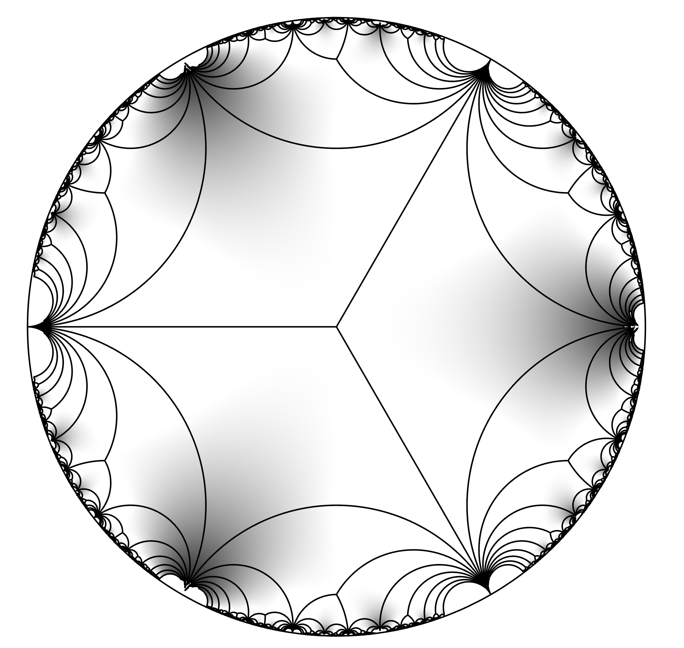
Lemma 5.2.6.

Let $\widetilde{s}\in\mathrm{PSL}_{2}(\mathbf{R})$ be a rotation of order $2N$ such that $\widetilde{s}^{2}=\widetilde{r}_{N}$ . Then

(5.2.7)

1-\widetilde{F}^{N}_{N}(\widetilde{s}\cdot\tau)=\frac{1}{1-\widetilde{F}^{N}_{N}(\tau)}.

Proof.

Recall our normalization of $\widetilde{F}_{N}$ that $\widetilde{F}_{N}(i)=0$ and $\widetilde{F}_{N}(i\infty)=1$ . By Corollary 5.2.4, $\tau=\pm\cot(\pi/2N)$ (in the same $\widetilde{\Phi}_{N}$ -orbit) is the other cusp of $\widetilde{\Phi}_{N}$ and thus $\widetilde{F}_{N}(\pm\cot(\pi/2N))=\infty$ . Moreover, both sides of (5.2.7) are uniformizers of $\mathbf{H}/\widetilde{\Phi}_{N}$ which take the value $0$ at the cusp $\cot(\pi/2N)$ and $\infty$ at the cusp $i\infty$ . This specifies them uniquely up to $x\mapsto\lambda x$ scalings. However, this last ambiguity is removed by noting that both sides are $1$ at $\tau=i$ . ∎

Remark 5.2.8.

The group $\widetilde{\Phi}_{N}$ is contained with index two in the larger group $\widetilde{\Psi}_{N}=\langle\widetilde{s},\widetilde{t}_{N}\rangle$ . The group $\widetilde{\Psi}_{N}$ has a fundamental domain consisting of the points $0,1,\zeta_{N}^{1/2}$ . But this is none other than a hyperbolic triangle with angles $\{\alpha,\beta,\gamma\}=\{\pi/N,0,0\}$ , whose conformal mapping from $\mathbf{H}$ is given by Schwarz triangle functions (see, for instance, [Car54, § 404 on page 185]). This suggests that $\widetilde{F}_{N}$ should directly be related to Schwarz triangle functions, which leads to a direct description of the inverse functions $\psi_{N}$ and $\varphi_{N}$ in terms of hypergeometric functions in Lemma 5.1.15.

In order to study the behavior of $\widetilde{F}_{N}$ near $x=1$ , we use the explicit formula for its inverse $\psi_{N}$ given in Lemma 5.1.15. The following lemma gives the asymptotic of the function $s_{N}$ used in formula of $\psi_{N}$ .

Lemma 5.2.9.

Fix a real constant $M_{0}>0$ . For $M\geq M_{0}$ and $|x|<e^{-MN}$ , we have the uniform estimate:

(5.2.10)

\left|\frac{s_{N}(1-x)}{\gamma_{N}}-(1-x)^{1/N}\frac{-\log x+2\gamma-2\psi(1/2+1/2N)}{-\log x+2\gamma-2\psi(1/2-1/2N)}\right|\ll\frac{|x|}{N},

where $\psi$ is the digamma function as in Lemma 5.1.19, and the implicit constant depends on $M_{0}$ but not on $N,M$ .

Proof.

By Lemma 5.1.19, we have for $a=1/2\pm 1/2N$ and $|x|<1$ the following equality:

(5.2.11)

\displaystyle{{}_{2}F_{1}{\left[\genfrac{.}{.}{0.0pt}{}{a\mskip 8.0mua}{2a};1-x\right]}=\frac{\Gamma(2a)}{\Gamma(a)^{2}}\sum_{k=0}^{\infty}\frac{(a)_{k}(a)_{k}}{k!^{2}}x^{k}\left(-\log{x}+2(\psi(k+1)-\psi(k+a))\right).}

We first prove that the coefficients in this power series are uniformly bounded. Since $|a|<1$ , we have $|(a)_{k}|/k!<1$ . Basic properties of the digamma function (cf. [AS92, 6.3.5, 6.3.14]) show that $\psi(x)$ is negative and strictly increasing for $0<x<1$ , and $|\psi(k)-\psi(k+a)|>|\psi(k+1)-\psi(k+1+a)|$ . Hence, $|\psi(k)-\psi(k+a)|$ is maximized when $k=1$ and $a=1/2-1/4$ . This immediately leads to the uniform estimates

\left|\sum_{k=1}^{\infty}\frac{(a)_{k}(a)_{k}}{k!^{2}}x^{k}\right|,\quad\left|\sum_{k=1}^{\infty}\frac{(a)_{k}(a)_{k}}{k!^{2}}x^{k}\left(2(\psi(k+1)-\psi(k+a))\right)\right|\ll|x|<e^{-MN}

For $|x|<e^{-MN}$ , we also have $\Re(\log{x})\leq-MN$ , and so in particular $|\log{x}|\geq MN$ regardless of the branch of logarithm. Combined with Lemma 5.1.15 and (5.2.11), this leads to the estimate

\frac{s_{N}(1-x)}{\gamma_{N}(1-x)^{1/N}}=\frac{-\log{x}+2\psi(1)-2\psi(1/2+1/2N)+O(x)}{-\log{x}+2\psi(1)-2\psi(1/2-1/2N)+O(x)}

where the implicit constants are uniform in $N$ , from which the result follows (using that $|\log{x}|\gg N$ ). ∎

Lemma 5.2.12.

Fix a pair of real positive numbers $M_{0}>0$ and $\epsilon>0$ . Consider any $M\geq M_{0}$ , and let $\widetilde{\Omega}^{\prime}_{N}\subset\mathbf{H}$ denote the fundamental domain for $\widetilde{\Phi}_{N}$ corresponding to $\Omega^{\prime}_{N}$ in Corollary 5.2.4. If $\tau\in\widetilde{\Omega}^{\prime}_{N}$ has

\|\widetilde{F}_{N}(\tau)^{N}-1\|<e^{-MN},

then

(5.2.13)

\Im(\tau)>\frac{2N^{2}M}{\pi^{2}}(1-\epsilon)

once $N\gg_{\epsilon,M_{0}}1$ , where the implicit constant depends only on $M_{0}$ and $\epsilon$ .

Proof.

By Corollary 5.2.4, $\widetilde{\Omega}^{\prime}_{N}$ is a fundamental domain of $\widetilde{F}^{N}_{N}$ and the only cusp where $\widetilde{F}_{N}^{N}=1$ is at $\tau=i\infty$ . So it suffices to consider $\widetilde{F}^{N}_{N}$ in a neighbourhood of the cusp $i\infty$ .

For $N$ sufficiently large, the inequality $\|\widetilde{F}_{N}(\tau)^{N}-1\|<e^{-MN}$ implies that $|\widetilde{F}_{N}(\tau)-1|<e^{-M(1-\varepsilon_{0})N}$ for some $\varepsilon_{0}$ that tends to zero as $N$ increases. Recall from the proof of Theorem 5.1.4 that $\psi_{N}(1)=1$ and hence $\widetilde{\psi}_{N}(1)=i\infty$ ; then it suffices to bound the imaginary part of

\tau=\widetilde{\psi}_{N}(1-x),\qquad\text{for }|x|<e^{-M(1-\varepsilon_{0})N}.

We may write this as

(5.2.14)

\tau=i\cdot\frac{1+\psi_{N}(1-x)}{1-\psi_{N}(1-x)}=i\cdot\frac{\gamma_{N}+s_{N}((1-x)^{N})}{\gamma_{N}-s_{N}((1-x)^{N})}.

Writing $1-X:=(1-x)^{N}$ , then the same estimate as above implies $|X|<e^{-M(1-2\varepsilon_{0})N}$ for sufficiently large $N$ . Thus we reduce the lemma to the estimate of

(5.2.15)

\tau=i\cdot\frac{\gamma_{N}+s_{N}(1-X)}{\gamma_{N}-s_{N}(1-X)},\quad|X|<e^{-M(1-2\varepsilon_{0})N}.

Now by Lemma 5.2.9 and [AS92, 6.3.7], we have

\tau=\frac{i\cot(\pi/2N)}{\pi}\left(2\gamma-\log{X}-\psi(1/2-1/2N)-\psi(1/2+1/2N)\right)+O(1),

where the implicit constant only depends on $M_{0}$ and $\varepsilon_{0}$ . The imaginary part of this does not depend on the choice of branch of $\log{X}$ and indeed only depends on $|X|$ , and we deduce with this approximation that

\Im(\tau)\geq\frac{\cot(\pi/2N)}{\pi}\left(2\gamma+NM(1-2\varepsilon_{0})-\psi(1/2-1/2N)-\psi(1/2+1/2N)\right)+O(1).

If we choose $\varepsilon_{0}:=\epsilon/2$ , then for $N\gg_{\epsilon,M_{0}}1$ this lower bound clearly exceeds

\frac{2N^{2}M(1-\epsilon)}{\pi^{2}}

as desired. ∎

The region (5.2.13) is a horoball for the cusp $i\infty$ in the upper half plane model $\mathbf{H}$ of the hyperbolic plane. Recall that in the Poincaré disc model $D(0,1)$ , the horoballs are the euclidean discs inside $D(0,1)$ which are tangent to the boundary circle. The following easy lemma describes how these horoballs transform under the hyperbolic isometry group.

Lemma 5.2.16.

Let $\mathcal{H}_{D}$ denote the image in the Poincaré disc model $D(0,1)$ of the horoball

\{\tau\in\mathbf{H}\,:\,\Im(\tau)\geq D\}

in the upper half plane model $\mathbf{H}$ . For $\gamma\in\mathrm{PSU}(1,1)$ with image $\widetilde{\gamma}=\begin{pmatrix}a&b\\ c&d\end{pmatrix}\in\mathrm{PSL}_{2}(\mathbf{R})$ , the image $\gamma\mathcal{H}_{D}$ of $\mathcal{H}_{D}$ under $\gamma$ in $D(0,1)$ is the disc with diameter

(5.2.17)

E(\gamma,D):=\frac{2}{1+D(a^{2}+c^{2})}

tangent to the boundary circle $\mathbf{T}$ at the point $(a-ic)/(a+ic)$ . ∎

We close this section by using Lemma 5.2.12 to derive a coarse yet fairly uniform upper bound on $\sup_{|z|=r}\log|F_{N}(z)|$ . Although not best-possible, it is enough as an input for the logarithmic error term in the Nevanlinna theory estimate in § 6.

Lemma 5.2.18.

For $N\gg 1$ and $r\in(0,1)$ , we have

\sup_{|z|=r}\log|F_{N}(z)|\ll\frac{N}{1-r},

where the implicit constants are both absolute.

Proof.

Set $S(M,N):=\{z\in D(0,1)\,:\,|F_{N}^{N}(z)-1|<e^{-MN}\}$ and $M:=\frac{N}{1-r}$ . Since $M\geq 2$ , we may take $M_{0}=2$ and $\epsilon=1/2$ in Lemma 5.2.12 and conclude that for $N\gg 1$ (with absolute implicit constant here), we have

S(M,N)\subset\bigcup_{\gamma\in\Phi_{N}}\gamma\mathcal{H}_{D},\quad\textrm{where }D=\frac{N^{2}M}{\pi^{2}}.

By Shimizu’s Lemma (see, for example, [EGM98, Theorem 3.1]) and Proposition 5.2.1, we have $2(|a|+|c|)\cot(\pi/2N)\geq 1$ for all $\widetilde{\gamma}=\left(\begin{matrix}a&b\\ c&d\end{matrix}\right)\in\widetilde{\Gamma}_{N}$ . Thus by Lemma 5.2.16,

E(\gamma,D)\leq 2D^{-1}(a^{2}+c^{2})\ll N^{-2}N^{-1}(1-r)N^{2}=\frac{1-r}{N},

where the implicit constant is absolute. Thus we have $E(\gamma,D)\leq 1-r$ for all $\gamma\in\Phi_{N}$ once $N^{-1}$ times the implicit constant is less than $1$ .

By Lemma 5.2.6, the set $\{z\in D(0,1)\,:\,|F_{N}(z)|>e^{M}+1\}$ is contained in $S(M,N)$ , which is contained in $D(0,1)\smallsetminus\overline{D(0,r)}$ by the above argument for $N\gg 1$ . Thus we conclude that

\sup_{|z|=r}\log|F_{N}(z)|\leq\log(e^{M}+1)\ll M=\frac{N}{1-r}.\qed

Remark 5.2.19.

A more refined bound is proved in Kraus–Roth [KR16, Theorems 1.2 and 1.10]. On the other hand, one can push our method further and prove, with rather more work but uniformly in $N\in\mathbf{N}_{>0}$ and $M\in[1,\infty)$ , that the supremum region $|F_{N}|<e^{M}$ is simply connected of conformal radius $1-O(M^{-2}N^{-3})$ from the origin; this is a sharp estimate. But taking for $\varphi$ in Corollary 2.0.5 the pullback of $F_{N}$ by the Riemann map of some such region $|F_{N}|<e^{M}$ , and ignoring thus the fine savings from the integrated bound (2.0.7) as opposed to the supremum, would only lead to an $O(N^{4})$ holonomy rank bound in place of our requisite logarithmically inflated bound $O(N^{3}\log{N})$ . In the next section we will see how to make the full use of the integrated holonomy bound, and use Nevanlinna’s value distribution theory to supply our final piece of the proof of the unbounded denominators conjecture.

6. Nevanlinna theory and uniform mean growth near the boundary

For our application of Corollary 2.0.5, we prove in this section the following uniform growth bound. Throughout this section, we assume as we may that $N\geq 2$ . Then the analytic map $F_{N}:D(0,1)\to\mathbf{P}^{1}$ omits the $N+1\geq 3$ values $\mu_{N}\cup\{\infty\}$ . In such a situation, we seek to exploit whatever growth constraints are imposed on the map by Nevanlinna’s value distribution theory. A theorem of Tsuji [Tsu52, Theorem 11] gives the general asymptotic

\int_{|z|=r}\log^{+}{|F|}\,\mu_{\mathrm{Haar}}=\frac{1}{N-1}\log{\frac{1}{1-r}}+O_{a_{1},\ldots,a_{N}}(1),

for any universal covering map $F:D(0,1)\to\mathbf{C}\smallsetminus\{a_{1},\ldots,a_{N}\}$ based at $F(0)=0$ (see also the discussion in Nevanlinna [Nev70, page 272]), however this is only asymptotically in $r\to 1^{-}$ for given punctures $\{a_{i}\}$ whereas we need a uniformity in both $r$ and $N$ . It is at the point (6.2.4) exploiting the small³³3Precisely, the relevant point of the specific puncture set $\{a_{1},\ldots,a_{N}\}\cup\{\infty\}=\mu_{N}\cup\{\infty\}$ in $\mathbf{P}^{1}\smallsetminus D(0,1)$ is that the degree- $N$ polynomial $\prod_{i=1}^{N}(x-a_{i})\in\mathbf{C}[x]$ has $N^{O(1)}$ coefficients. coefficients of $\prod_{\zeta\in\mu_{N}}(x-\zeta)=x^{N}-1$ that our argument below makes a critical use of the special feature of the target set $\mu_{N}\cup\{\infty\}$ of omitted values.

Theorem 6.0.1.

For each of the choices

p(x)\in\big{\{}x^{N},x^{N}/(x^{N}-1),\,1/(x^{N}-1)\big{\}},

we have uniformly in $N\in\mathbf{N}_{>0}$ and $r\in(0,1)$ the mean growth bound

(6.0.2)

\int_{|z|=r}\log^{+}|p\circ F_{N}|\,\mu_{\mathrm{Haar}}\ll\log{\frac{N}{1-r}},

with some (effectively computable) absolute implicit constant.

6.1. Preliminaries in Nevanlinna theory

This section collects some standard material from Nevanlinna’s value distribution theory. The reader should feel encouraged to skip this part on a first reading, and refer back as necessary.

6.1.1. The Nevanlinna characteristic

The left-hand side of (6.0.2) is known as the mean proximity function at $\infty$

m(r,f)=m(r,f;\infty):=\int_{|z|=r}\log^{+}{|f|}\,\mu_{\mathrm{Haar}}\in[0,\infty).

It is complemented by the counting function

N(r,f)=N(r,f;\infty):=\sum_{\rho\,:\,0<|\rho|<r}\mathrm{ord}_{\rho}^{-}(f)\log{\frac{r}{|\rho|}}+\mathrm{ord}_{0}^{-}(f)\,\log{r},

where, in general for a meromorphic mapping $f:D(0,1)\to\mathbf{P}^{1}$ , we denote by $\mathrm{ord}_{\rho}^{-}(f):=\mathrm{ord}^{+}(1/f)=\max(0,\mathrm{ord}(1/f))$ the pole order (if $\rho$ is a pole, and $0$ if $f$ is holomorphic at $\rho$ ).

The Nevanlinna characteristic function

T(r,f):=m(r,f)+N(r,f)

is the well-behaved quantity functorially.

Lemma 6.1.2.

For every meromorphic function $f:D(0,1)\to\mathbf{P}^{1}$ regular at $0$ (that is: with $f(0)\neq\infty$ ), and for every $r\in(0,1)$ , we have

N(r,f)\geq 0,

with equality if and only if $f$ is holomorphic (has no poles) throughout the disc $D(0,r)$ .

The Nevanlinna characteristic function $T(r,f)$ satisfies for every $a\in\mathbf{C}$ the relation

(6.1.3)

|T(r,f)-T(r,1/(f-a))-\log{|c(f,a)|}|\leq\log^{+}{|a|}+\log{2},

where

c(f,a):=\lim_{z\to 0}(f(z)-a)z^{-\mathrm{ord}_{0}(f-a)}.

Proof.

This is Rolf Nevanlinna’s first main theorem, and is proved formally and straightforwardly from the Poisson–Jensen formula (see, for instance, [BG06, Proposition 13.2.6]), which we may rewrite as

(6.1.4)

T(r,f)-T(r,1/f)=\log|c(f,0)|,

and the triangle inequality relation

(6.1.5)

\big{|}\log^{+}{|f-a|}-\log^{+}{|f|}\big{|}\leq\log^{+}{|a|}+\log{2}.

See Hayman [Hay64, Theorem 1.2] or Bombieri–Gubler [BG06, Theorem 13.2.10] for the details. We note that $c(f,a)=f(0)-a$ when $a\neq f(0)$ . ∎

6.1.6. The lemma on the logarithmic derivative

The lemma on the logarithmic derivative—a strong explicit form of which is cited in (6.1.14) below—is the centerpiece of Rolf Nevanlinna’s original analytic proof of his second main theorem of value distribution theory. The logarithmic error feature of this sharp upper bound on the proximity function of a logarithmic derivative enables us to derive Theorem 6.0.1 from the relatively crude supremum growth bound in Lemma 5.2.18.

The reader willing to take (6.1.14) for granted may at this point proceed directly to § 6.2. Nevertheless, since the proof simplifies considerably in the case that we need of a functional unit (a nowhere vanishing holomorphic function), we include our own self-contained treatment of a basic explicit case of the lemma on the logarithmic derivative.

Lemma 6.1.7.

Let $g:\overline{D(0,R)}\to\mathbf{C}^{\times}$ be a nowhere vanishing holomorphic function on some open neighborhood of the closed disc $|z|\leq R$ . Assume that $g(0)=1$ . Then, for all $0<r<R$ ,

(6.1.8)

m\Big{(}r,\frac{g^{\prime}}{g}\Big{)}<\log^{+}{\Big{\{}\frac{m(R,g)}{r}\frac{R}{R-r}\Big{\}}}+\log{2}+1/e.

Proof.

Our functional unit assumption means that the function $\log{g(z)}$ has a single valued holomorphic branch on a neighborhood of the closed disc $|z|\leq R$ with $\log{g(0)}=0$ . Its real part is the harmonic function $\log{|g(z)|}$ . Poisson’s formula on the harmonic extension of a continuous function from the boundary to the interior of a disc reads

(6.1.9)

\log{|g(z)|}=\int_{|w|=R}\log{|g(w)|}\cdot\mathfrak{R}\Big{(}\frac{w+z}{w-z}\Big{)}\,\mu_{\mathrm{Haar}}(w),

where $k(z,w):=\mathfrak{R}\Big{(}\frac{w+z}{w-z}\Big{)}$ is the Poisson kernel. This formula in fact upgrades to

(6.1.10)

\log{g(z)}=\int_{|w|=R}\log{|g(w)|}\cdot\frac{w+z}{w-z}\,\mu_{\mathrm{Haar}}(w),

because both sides are holomorphic in $z$ , have identical real parts, and evaluate to zero at $z=0$ .

Differentiation in the integrand of (6.1.10) gives a reproducing kernel for our logarithmic derivative as well:

(6.1.11)

\frac{g^{\prime}(z)}{g(z)}=\int_{|w|=R}\frac{2w}{(w-z)^{2}}\log{|g(w)|}\,\mu_{\mathrm{Haar}}(w),\qquad z\in D(0,R).

for the logarithmic derivative in the interior of the disc $|z|\leq R$ in terms of boundary values on the circle $|z|=R$ . We have the elementary calculation

(6.1.12)

\int_{|z|=r}|w-z|^{-2}\,\mu_{\mathrm{Haar}}(z)=\frac{1}{R^{2}-r^{2}}\quad\textrm{ for }|w|=R>r,

and thus the $|z|=r$ integral of (6.1.11) with the triangle inequality and interchanging the orders of the integrations and using $|\log{|g|}|=\log^{+}{|g|}+\log^{-}{|g|}=\log^{+}{|g|}+\log^{+}{|1/g|}$ yields

\begin{split}\int_{|z|=r}\Big{|}\frac{g^{\prime}(z)}{g(z)}\Big{|}\,\mu_{\mathrm{Haar}}\leq 2R\int_{|z|=r}\int_{|w|=R}|w-z|^{-2}\,\big{|}\log{|g(w)|}\big{|}\,\mu_{\mathrm{Haar}}(w)\,\mu_{\mathrm{Haar}}(z)\\ =2R\int_{|w|=R}\Big{(}\int_{|z|=r}|w-z|^{-2}\,\mu_{\mathrm{Haar}}(z)\Big{)}\,\big{|}\log{|g(w)|}\big{|}\,\mu_{\mathrm{Haar}}(w)\\ =\frac{2R}{R^{2}-r^{2}}\int_{|w|=R}\big{|}\log{|g(w)|}\big{|}\,\mu_{\mathrm{Haar}}(w)\\ =\frac{2R}{R^{2}-r^{2}}\Big{(}m(R,g)+m(R,1/g)\Big{)}=\frac{4R\,m(R,g)}{R^{2}-r^{2}},\end{split}

on using on the final line the harmonicity property again which implies

\int_{|w|=R}\log{|g|}\,\mu_{\mathrm{Haar}}(w)=\log{|g(0)|}=0.

The final piece of the proof borrows from [BK01, section 4]. Let

E:=\Big{\{}z\,:\,|z|=r,\,|g^{\prime}(z)/g(z)|>1\Big{\}},

a measurable subset of the circle $|z|=r$ . Since the function $\log^{+}{|x|}$ is concave on $x\in[1,\infty)$ where it coincides with $\log{|x|}$ , Jensen’s inequality gives

\begin{split}\int_{|z|=r}\log^{+}{\Big{|}\frac{g^{\prime}}{g}\Big{|}}\,\mu_{\mathrm{Haar}}\leq\mu_{\mathrm{Haar}}(E)\log^{+}\Big{(}\frac{1}{\mu_{\mathrm{Haar}}(E)}\int_{E}\Big{|}\frac{g^{\prime}(z)}{g(z)}\Big{|}\,\mu_{\mathrm{Haar}}(z)\Big{)}\\ \leq\mu_{\mathrm{Haar}}(E)\log^{+}\Big{(}\frac{1}{\mu_{\mathrm{Haar}}(E)}\int_{|z|=r}\Big{|}\frac{g^{\prime}(z)}{g(z)}\Big{|}\,\mu_{\mathrm{Haar}}(z)\Big{)}\\ \leq\mu_{\mathrm{Haar}}(E)\log^{+}\Big{(}\int_{|z|=r}\Big{|}\frac{g^{\prime}(z)}{g(z)}\Big{|}\,\mu_{\mathrm{Haar}}(z)\Big{)}+\mu_{\mathrm{Haar}}(E)\log(1/\mu_{\mathrm{Haar}}(E))\\ \leq\log^{+}\int_{|z|=r}\Big{|}\frac{g^{\prime}(z)}{g(z)}\Big{|}\,\mu_{\mathrm{Haar}}(z)+\sup_{t\in(0,1]}\big{\{}t\log{(1/t)}\big{\}}\\ \leq\log^{+}{\Big{\{}\frac{4R\,m(R,g)}{R^{2}-r^{2}}\Big{\}}}+\frac{1}{e}\leq\log^{+}{\Big{\{}\frac{m(R,g)}{r}\frac{R}{R-r}\Big{\}}}+\log{2}+\frac{1}{e},\end{split}

using $R^{2}-r^{2}=(R+r)(R-r)>2r(R-r)$ on the final line. ∎

Remark 6.1.13.

The case of arbitrary meromorphic functions $g:\overline{D(0,R)}\to\mathbf{P}^{1}$ is handled similarly by a differentiation in the general Poisson–Jensen formula, but with rather more work to estimate the finite sum over the zeros and poles of $g$ . See for instance [Nev70, § IX.3.1, page 244, (3.2)] or [Hay64, Lemma 2.3 on page 36] for similar bounds. By using a technique due to Kolokolnikov for handling the sum over the zeros and poles, Goldberg and Grinshtein [GG76] obtained the general bound

(6.1.14)

m\Big{(}r,\frac{g^{\prime}}{g}\Big{)}<\log^{+}{\Big{\{}\frac{T(R,g)}{r}\frac{R}{R-r}\Big{\}}}+5.8501,\quad\textrm{for }g(0)=1,

and proved that it is essentially best-possible in form apart for the value of the free numerical constant $5.8501$ (that has since been somewhat further reduced in the literature, see Benbourenane–Korhonen [BK01]). The paper of Hinkkanen [Hin92] and the books of Cherry–Ye [CY01] and Ru [Ru21] discuss the implications to the structure of the error term in Nevanlinna second main theorem, mirroring Osgood and Vojta’s dictionary to Diophantine approximation and comparing to Lang’s conjecture modeled on Khinchin’s theorem.

6.2. Proof of Theorem 6.0.1

For $f:D(0,1)\to\mathbf{C}$ holomorphic, the polar divisor is empty, and so $N(r,f)=0$ and $m(r,f)=T(r,f)$ . Since by definition $F_{N}^{N}-1$ is a unit in the ring of holomorphic functions on $D(0,1)$ , our requisite bound (6.0.2) rewrites in Nevanlinna notation into

(6.2.1)

T(r,p\circ F_{N})\ll\log{\frac{N}{1-r}},\quad\textrm{for each of }p(x)\in\big{\{}x^{N}/(x^{N}-1),\,1/(x^{N}-1),\,x^{N}\big{\}}.

6.2.2. Equivalence of bounds for different $p(x)$

By Lemma 6.1.2, the fact $x^{N}/(x^{N}-1)=1+1/(x^{N}-1)$ , and (6.1.5), the three cases for $p(x)$ are equivalent to one another. Here we give the explicit estimate in one direction, which will be used later:

(6.2.3)

\begin{split}T(r,p\circ F_{N})=m\Big{(}r,1+\frac{1}{F_{N}^{N}-1}\Big{)}\geq m\Big{(}r,\frac{1}{F_{N}^{N}-1}\Big{)}-\log{2}\\ =T\Big{(}r,\frac{1}{F_{N}^{N}-1}\Big{)}-\log{2}=T(r,F_{N}^{N}-1)-\log{2}\\ \geq T(r,F_{N}^{N})-2\log{2}=N\,T(r,F_{N})-\log{4},\end{split}

where we use $F_{N}(0)=0$ and $F_{N}^{N}-1$ is a unit in the ring of holomorphic functions on $D(0,1)$ . In the rest of this subsection, we will prove Theorem 6.0.1 in the form $T(r,F_{N}^{N})\ll\log{\frac{N}{1-r}}$ but pivoting around the choice

(6.2.4)

p(x):=\frac{x^{N}}{x^{N}-1}=\frac{x}{N}\sum_{\zeta\in\mu_{N}}\frac{1}{x-\zeta}.

6.2.5. Reduction to a logarithmic derivative

By either the chain rule or the partial fractions decomposition, we see that the logarithmic derivative $f^{\prime}/f$ of the nowhere vanishing holomorphic function

(6.2.6)

f:=1-F_{N}^{N}\quad:\quad D(0,1)\to\mathbf{C}^{\times}

is related to $p\circ F_{N}=F_{N}^{N}/(F_{N}^{N}-1)$ by

(6.2.7)

p\circ F_{N}=\frac{F_{N}}{NF_{N}^{\prime}}\frac{f^{\prime}}{f}.

The idea then is that the piece $f^{\prime}/f$ in the decomposition (6.2.7) is small on average over circles by the lemma on the logarithmic derivative (Corollary 6.2.9 below), while—again by the lemma on the logarithmic derivative, in Corollary 6.2.11 below—the characteristic functions of $p\circ F_{N}$ and $F_{N}/F_{N}^{\prime}$ are equal respectively to $NT(r,F_{N})$ and $T(r,F_{N})$ up to a small error.

6.2.8. Two corollaries of the lemma on the logarithmic derivative

Corollary 6.2.9.

For $f=1-F_{N}^{N}$ , we have

(6.2.10)

m\Big{(}r,\frac{f^{\prime}}{f}\Big{)}\ll\sup_{|z|=(1+r)/2}\log^{+}{\log{|F_{N}|}}+\log{\frac{N}{1-r}}.

Proof.

By applying Lemma 6.1.7 to $f$ and the outer radius choice $R:=1-(1-r)/2=(1+r)/2$ , and using (cf. [BG06, Corollary 13.2.14]) that $m(r,f^{\prime}/f)=T(r,f^{\prime}/f)$ is a monotone increasing function of $r$ , we find the mean growth bound

\begin{split}m\Big{(}r,\frac{f^{\prime}}{f}\Big{)}\ll\log^{+}{T\Big{(}\frac{1+r}{2},f\Big{)}}+\log{\frac{e}{1-r}}\\ =\log^{+}{m\Big{(}\frac{1+r}{2},1-F_{N}^{N}\Big{)}}+\log{\frac{e}{1-r}}\\ \ll\log^{+}{m\Big{(}\frac{1+r}{2},F_{N}^{N}\Big{)}}+\log{\frac{e}{1-r}}\\ \ll\log^{+}{m\Big{(}\frac{1+r}{2},F_{N}\Big{)}}+\log{\frac{N}{1-r}}\\ \ll\sup_{|z|=(1+r)/2}\log^{+}{\log{|F_{N}|}}+\log{\frac{N}{1-r}},\end{split}

where in the last step we have estimated a mean proximity function trivially by a supremum function. ∎

Corollary 6.2.11.

We have

(6.2.12)

m\Big{(}r,\frac{F_{N}}{F_{N}^{\prime}}\Big{)}\leq T(r,F_{N})+O\Big{(}\log^{+}{\frac{N}{1-r}}+\sup_{|z|=(1+r)/2}\log^{+}{\log{|F_{N}|}}\Big{)}.

The idea of the proof is to combine Lemma 6.1.7 applied to the functional unit $1-F_{N}$ and the standard chain of implications based on Jensen’s formula in the reduction of the second main theorem to the lemma on the logarithmic derivative (see, for example, [Hay64, pages 33–34]).

Proof.

By (6.1.4) for the function $F_{N}^{\prime}/F_{N}$ , and the fact that $F_{N}$ is holomorphic on the disc $D(0,1)$ with $F_{N}(0)=0$ and $F_{N}^{\prime}(0)\neq 0$ , we have:

(6.2.13)

\begin{split}m\Big{(}r,\frac{F_{N}}{F_{N}^{\prime}}\Big{)}=m\Big{(}r,\frac{F_{N}^{\prime}}{F_{N}}\Big{)}+N\Big{(}r,\frac{F_{N}^{\prime}}{F_{N}}\Big{)}-N\Big{(}r,\frac{F_{N}}{F_{N}^{\prime}}\Big{)}-\log{c(F_{N}^{\prime}/F_{N},0)}\\ =m\Big{(}r,\frac{F_{N}^{\prime}}{F_{N}}\Big{)}+N\Big{(}r,1/F_{N}\Big{)}-N\Big{(}r,F_{N}\Big{)}-N\Big{(}r,1/F_{N}^{\prime}\Big{)}+N\Big{(}r,F_{N}^{\prime}\Big{)}\\ =m\Big{(}r,\frac{F_{N}^{\prime}}{F_{N}}\Big{)}+N\Big{(}r,1/F_{N}\Big{)}-N\Big{(}r,1/F_{N}^{\prime}\Big{)}=m\Big{(}r,\frac{F_{N}^{\prime}}{F_{N}}\Big{)}+N\Big{(}r,1/F_{N}\Big{)}.\end{split}

Here for the last equality we recall that $F_{N}:D(0,1)\to\mathbf{C}\smallsetminus\mu_{N}$ is an étale analytic mapping, hence the derivative $F_{N}^{\prime}$ is nowhere vanishing.

We continue to estimate with the triangle inequality (for the second and third lines) and then (6.1.4), noting that $|F^{\prime}_{N}(0)|>1$ (for the inequality in the fourth line):

\begin{split}m\Big{(}r,\frac{F_{N}}{F_{N}^{\prime}}\Big{)}=m\Big{(}r,\frac{F_{N}^{\prime}}{F_{N}}\Big{)}+N\Big{(}r,1/F_{N}\Big{)}\\ \leq m\Big{(}r,\frac{F_{N}^{\prime}}{1-F_{N}}\Big{)}+m\Big{(}r,\frac{1-F_{N}}{F_{N}}\Big{)}+N\Big{(}r,1/F_{N}\Big{)}\\ \leq m\Big{(}r,\frac{F_{N}^{\prime}}{1-F_{N}}\Big{)}+\log 2+m\Big{(}r,\frac{1}{F_{N}}\Big{)}+N\Big{(}r,1/F_{N}\Big{)}\\ =m\Big{(}r,\frac{(1-F_{N})^{\prime}}{1-F_{N}}\Big{)}+T(r,1/F_{N})+\log 2\leq m\Big{(}r,\frac{(1-F_{N})^{\prime}}{1-F_{N}}\Big{)}+T(r,F_{N})+\log 2\\ \leq T(r,F_{N})+O\Big{(}\log^{+}{\frac{N}{1-r}}+\sup_{|z|=(1+r)/2}\log^{+}{\log{|F_{N}|}}\Big{)},\end{split}

upon again using Lemma 6.1.7 with $R:=(1-r)/2$ but now for the functional unit $g=1-F_{N}$ , and a similar argument as in the proof of Corollary 6.2.9. ∎

6.2.14. Completing the proof from the crude supremum bound in Lemma 5.2.18

At this point the key identity (6.2.7) allows us to combine the estimates (6.2.10) and (6.2.12), arriving at the uniform bound

(6.2.15)

\begin{split}T(r,p\circ F_{N})=m(r,p\circ F_{N})\leq m\Big{(}r,\frac{f^{\prime}}{f}\Big{)}+m\Big{(}r,\frac{F_{N}}{F_{N}^{\prime}}\Big{)}\\ \leq T(r,F_{N})+O\Big{(}\log^{+}{\frac{N}{1-r}}+\sup_{|z|=(1+r)/2}\log^{+}{\log{|F_{N}|}}\Big{)}.\end{split}

We leverage the upper bound (6.2.15) on $T(r,p\circ F_{N})=N\,T(r,F_{N})+O(1)$ against the lower bound (6.2.3) and get a uniform upper bound on $T(r,F_{N})$ :

(6.2.16)

(N-1)T(r,F_{N})\ll\log^{+}{\frac{N}{1-r}}+\sup_{|z|=(1+r)/2}\log^{+}{\log{|F_{N}|}}.

Upon doubling the absolute implicit constant, plainly for $N\geq 2$ this is equivalent to

T(r,F_{N}^{N})=NT(r,F_{N})\ll\log^{+}{\frac{N}{1-r}}+\sup_{|z|=(1+r)/2}\log^{+}{\log{|F_{N}|}},

uniformly in all $N\geq 2$ and $r\in(0,1)$ .

Hence Theorem 6.0.1 follows from Lemma 5.2.18 upon replacing $r$ there with $(1+r)/2$ .

6.2.17. A historical note

The bound (6.2.16) can be compared to the well-known particular case for entire holomorphic functions of the classical Nevanlinna second main theorem (whose method of proof we emulate here), stating that for any entire function $g:\mathbf{C}\to\mathbf{C}$ , and any $N$ -tuple of pairwise distinct points $a_{1},\ldots,a_{N}\in\mathbf{C}$ , the Nevanlinna characteristic $T(r,g)=m(r,g)=\int_{|z|=r}\log^{+}{|g|}\,\mu_{\mathrm{Haar}}$ satisfies the upper bound

(6.2.18)

(N-1)T(r,g)+N_{\mathrm{ram}}(r,g)\leq\sum_{i=1}^{N}N(r,a_{i})+O(\log{T(r,g)})+O(\log{r})

outside of an exceptional set of radii $r\in E\subset[0,\infty)$ of finite Lebesgue measure: $m(E)<\infty$ . Here $N_{\mathrm{ram}}(r,g)=N(r,1/g^{\prime})$ is a ramification term, which is always nonnegative and vanishes if the map $g$ is étale. This is Nevanlinna’s quantitative strengthening of Picard’s theorem on at most one omitted value for a nonconstant entire function, for if each of $a_{1},\ldots,a_{N}$ is omitted then all counting terms $N(r,a_{i})=0$ vanish on the right-hand side of (6.2.18), leading if $N\geq 2$ to an $O(\log{r})$ upper bound on the growth $T(r,g)$ of $g$ . The idea is that we similarly have a holomorphic map $F_{N}$ omitting the $N$ values $a_{h}=\exp(2\pi ih/N)$ , except $F_{N}$ is on a disc rather than the entire plane, and that (6.2.18) largely extends as a growth bound for holomorphic maps on a disc. For such completely quantitative results we refer the reader to Hinkkanen [Hin92, Theorem 3] or Cherry–Ye [CY01, Theorem 4.2.1 or Theorem 2.8.6]. We cannot directly apply these general theorems in their verbatim forms as they only lead to a bound of the form $m(r,F_{N})\ll\frac{1}{N}\log{\frac{1}{1-r}}+\log{N}$ in place of the required $m(r,F_{N})\ll\frac{1}{N}\log{\frac{N}{1-r}}$ ; cf. the term $(q+1)\log(q/\delta)$ in [Hin92, line (1.24)], where $q=N$ signifies the number of targets $a_{i}$ . But fortuitously we were able to modify their proofs by making an additional use of the key pivot relation (6.2.4) particular to our situation of $\{a_{1},\ldots,a_{q}\}=\mu_{N}$ .

For our case of functions on the disc, we compare to [Hay64, Theorem 2.1]. For holomorphic $f$ , we again have the ramification term $N_{\mathrm{ram}}(r,f)=N(r,1/f^{\prime})$ (this term is denoted by $N_{1}(r)$ in [Hay64]), which is always nonnegative. In (6.2.13), even without using the étaleness of $F_{N}$ , one would drop the ramification term by positivity and still obtain the requisite bound $\displaystyle m\Big{(}r,\frac{\varphi}{\varphi^{\prime}}\Big{)}\leq m\Big{(}r,\frac{\varphi^{\prime}}{\varphi}\Big{)}+N\Big{(}r,1/\varphi\Big{)}$ . In this way, our treatment also recovers the bound $\int_{|z|=r}\log^{+}{|\varphi|}\,\mu_{\mathrm{Haar}}\leq\frac{1}{N-1}\log{\frac{1}{1-r}}+O_{\varphi}(1)$ for every holomorphic map $\varphi:D(0,1)\to\mathbf{C}\smallsetminus\mu_{N}$ avoiding the $N$ -th roots of unity (which is not necessarily the universal covering map).

6.3. Proof of Theorem 1.0.1

At this point we have established all the pieces for the proof of our main result. By Theorem 5.1.4, assumption (1) in Proposition 3.0.1 is indeed satisfied, with the sharp constant $A:=\zeta(3)/2>0$ . By Theorem 6.0.1 with the choices $p(x):=x^{N}$ and $r:=1-BN^{-3}$ , assumption (2) in Proposition 3.0.1 is also satisfied. In terms of the algebras of modular forms $M_{2N}$ and $R_{2N}$ at an even Wohlfahrt level $2N$ introduced in 4.2.1, the conclusion of Proposition 3.0.1 is thus an inequality $[R_{2N}:M_{2}]\leq CN^{3}\log{N}$ , for some absolute implicit constant $C\in\mathbf{R}$ independent of $N$ . At this point Proposition 4.3.5 proves the equality $R_{2N}=M_{2N}$ for all $N\in\mathbf{N}_{>0}$ , which is the unbounded denominators conjecture.

The proof of Theorem 1.0.1 is thus completed. ∎

Remark 6.3.1.

Our proof for Theorem 1.0.1 generalizes in the obvious way to establish that a modular form $f(\tau)$ having a Fourier expansion in $\overline{\mathbf{Z}}\llbracket q^{1/N}\rrbracket$ (algebraic integer Fourier coefficients) at one cusp, and meromorphic at all cusps, is a modular form for a congruence subgroup of $\mathrm{SL}_{2}(\mathbf{Z})$ . We include an indication of the details.

Since $f(\tau)$ is a modular form, we are reduced to the situation of a number field $K$ such that $f(\tau)\in O_{K}\llbracket q^{1/N}\rrbracket$ . We use $R_{2N}$ to denote the $K(\lambda)$ -algebra generated by modular functions with coefficients in $K$ , bounded denominators at $\zeta=i\infty$ , and cusp widths dividing $2N$ at all cusps $\zeta\in\mathbf{P}^{1}(\mathbf{Q})$ (similar to Definition 4.2.1). We follow the proof of Proposition 3.0.1 now on the case of the $K(\lambda)$ -vector space $\mathcal{V}(U,x(t),O_{K})$ from Definition 2.0.4. Then $R_{2N}\subset\mathcal{V}(U,x(t),O_{K})$ . Note that $U$ is stable under the action of $\mathrm{Gal}(\overline{\mathbf{Q}}/\mathbf{Q})$ , and thus $\mathcal{V}(U,x(t),O_{K})=\mathcal{V}(U,x(t),\mathbf{Z})\otimes_{\mathbf{Q}}K$ and $\dim_{K(\lambda)}\mathcal{V}(U,x(t),O_{K})=\dim_{\mathbf{Q}(\lambda)}\mathcal{V}(U,x(t),\mathbf{Z})$ . Thus by Corollary 2.0.5, Theorem 5.1.4, and Theorem 6.0.1, we still have that $R_{2N}$ has dimension at most $CN^{3}\log N$ over $K(\lambda)$ . The claimed extension to $\overline{\mathbf{Z}}\llbracket q^{1/N}\rrbracket$ Fourier expansions now follows upon remarking that the proof of Proposition 4.3.5 still persists when $\mathbf{Q}$ is replaced by $K$ .

Remark 6.3.2.

It is also possible to derive the $\bar{\mathbf{Z}}\llbracket q^{1/N}\rrbracket$ generalization directly from Theorem 1.0.1, by the following argument pointed out to us by John Voight. The absolute Galois group $\mathrm{Gal}(\bar{\mathbf{Q}}/\mathbf{Q})$ acts on the $q$ -expansions of modular forms. If $f(\tau)\in O_{K}\llbracket q^{1/N}\rrbracket$ is a modular form on a finite index subgroup of $\mathrm{SL}_{2}(\mathbf{Z})$ , and $\alpha_{1},\ldots,\alpha_{d}$ is a $\mathbf{Z}$ -basis of $O_{K}$ , then $f_{i}(\tau):=\mathrm{Tr}_{K/\mathbf{Q}}(\alpha_{i}f(\tau))\in\mathbf{Z}\llbracket q^{1/N}\rrbracket$ for each $i=1,\ldots,d$ . Theorem 1.0.1 gives that each $f_{i}(\tau)$ is modular for some congruence subgroup, say $\Gamma_{i}$ . At this point $f(\tau)$ , being a $K$ -linear combination of $f_{1},\ldots,f_{d}$ , is modular for the congruence subgroup $\Gamma_{1}\cap\cdots\cap\Gamma_{d}$ .

7. Generalization to vector-valued modular forms

7.1. Generalized McKay–Thompson series with roots from monstrous moonshine

Our argument also proves a vector generalization of the unbounded denominators conjecture, which has been conjectured by Mason [Mas12] (see also the earlier work of Kohnen and Mason [KM08] for a special case) to the setting of vector-valued modular forms of $\mathrm{SL}_{2}(\mathbf{Z})$ , with motivation from the theory of vertex operator algebras and the monstrous moonshine conjectures. The weaker statement of algebraicity over the ring of modular forms was conjectured earlier by Anderson and Moore [AM88], within the context of the partition functions or McKay–Thompson series attached to rational conformal field theories. We refer also to André [And04, Appendix] for a discussion from the arithmetic algebraization point of view — the method that we build upon in our present paper — on the Grothendieck–Katz $p$ -curvature conjecture. Eventually the more precise expectation crystallized (see Eholzer [Eho95, Conjecture on page 628]) that all rational conformal field theory graded twisted characters are in fact classical modular forms for a congruence subgroup of $\mathrm{SL}_{2}(\mathbf{Z})$ , which is more precise than Anderson and Moore’s conjectured algebraicity over the modular ring $\mathbf{Z}[E_{4},E_{6}]$ .

This conjecture became known as the congruence property in conformal field theory, and was proved in the eponymous paper of Dong, Lin and Ng [DLN15], after landmark progresses from many authors (for some history, including notably Bantay’s solution [Ban03] under a certain heuristic assumption, the orbifold covariance principle [Ban00, Ban02, Xu06], we refer the reader to the introduction of [DLN15]). Finally, the congruence property for the McKay–Thompson series in the full equivariant setting (orbifold theory) $V^{G}$ of a finite group $G$ of automorphisms of a rational, $C_{2}$ -cofinite vertex operator algebra $V$ (the prime example being the Fischer–Griess Monster group operating on the moonshine module of Frenkel–Lepowski–Meurman [FLM88]) was proved by Dong and Ren [DR18] by a reduction to the special case $G=\{1\}$ that is [DLN15].

Our paper, via Theorem 7.3.3 below for the vector valued extension of the congruence property, inherits a new proof of these modularity theorems. The connection was engineered by Knopp and Mason [KM03a], with their formalization of generalized modular forms for $\mathrm{SL}_{2}(\mathbf{Z})$ , and fine tuned by Kohnen and Mason [KM08, § 4], who brought forward the idea of a purely arithmetic approach — based on the integrality properties of the Fourier coefficients, that record a graded dimension and are hence integers — for a part of Borcherds’ theorem [Bor92] (the Conway–Norton “monstrous moonshine” conjecture). Namely, suppressing the Hauptmodul property, for the classical modularity — under a congruence subgroup of $\mathrm{SL}_{2}(\mathbf{Z})$ — of all the various McKay–Thompson series for the Monster group over the moonshine module $V^{\sharp}$ . Whereas Borcherds’ proof, based on his own generalized Kac–Moody algebras that go outside of the general framework of vertex operator algebras, is rather particular to the Monster vertex algebra and genus $0$ arithmetic groups, Kohnen and Mason proposed that an arithmetic abstraction from the integrality of Fourier coefficients might open up a window on the modularity and congruence properties to apply just as well in the equivariant setting to any rational $C_{2}$ -cofinite vertex operator algebra — this theorem, eventually proved in [DLN15, DR18] by other means, was an open problem at the time of [KM08].

It is precisely this arithmetic scheme that we are able to complete with our paper.

7.2. Unbounded denominators for the solutions of certain ODEs

In the language of Anderson–Moore [AM88, page 445], the functions occurring below are said to be quasi-automorphic for the modular group $\mathrm{PSL}_{2}(\mathbf{Z})$ , while in Knopp–Mason [KM03b] or Gannon [Gan14], they arise as component functions of vector-valued modular forms for $\mathrm{SL}_{2}(\mathbf{Z})$ . We firstly take up the holonomic viewpoint and give a yet another formulation, in the equivalent language of linear ODEs on the triply punctured projective line, where we think of $x$ as the modular function $\lambda(\tau)/16\in q+q^{2}\mathbf{Z}\llbracket q\rrbracket$ , where $q=\exp(\pi i\tau)$ , and of $\mathbf{P}^{1}\smallsetminus\{0,1/16,\infty\}$ as the modular curve $Y(2)=\mathbf{H}/\Gamma(2)$ . This answers the question raised in [And04, Appendix, A.5]. For simplicity of exposition, we only consider the case of a power series expansion $f(x)\in\mathbf{Z}\llbracket x\rrbracket$ here, as opposed to a general Puiseux expansion (see Remark 7.2.2).

Theorem 7.2.1.

Let $f(x)\in\mathbf{Z}\llbracket x\rrbracket$ be an integer coefficients formal power series solution of $L(f)=0$ , where $L$ is a linear differential operator without singularities⁴⁴4Similarly to 2.0.4, the proof allows for singularities on $\mathbf{P}^{1}\smallsetminus\{0,1/16,\infty\}$ provided their local monodromy is trivial. on $\mathbf{P}^{1}\smallsetminus\{0,1/16,\infty\}$ . If the $x=0$ local monodromy of $L$ is finite, then $f(x)$ is algebraic, and more precisely, the function $f(\lambda(\tau)/16)$ on $\mathbf{H}$ is automorphic for some congruence subgroup $\Gamma(N)$ of $\mathrm{SL}_{2}(\mathbf{Z})$ .

Proof.

Our condition is that the $x=0$ local monodromy group is $\mathbf{Z}/N$ for some $N\in\mathbf{N}_{>0}$ . Then the formal function $g(x):=f(x^{N})$ is in $\mathbf{Z}\llbracket x\rrbracket$ and fulfills a linear ODE on $\mathbf{P}^{1}\smallsetminus\{16^{-1/N}\mu_{N},\infty\}$ . In our notation of Corollary 2.0.5, that means $g\in\mathcal{H}(\mathbf{C}\smallsetminus 16^{-1/N}\mu_{N},\mathbf{Z})$ . Hence, denoting again by $F_{N}:D(0,1)\to\mathbf{C}\smallsetminus\mu_{N}$ the universal covering map taking $F_{N}(0)=0$ , recalling our exact uniformization radius formula in Theorem 5.1.4 giving in particular the strict lower bound

|F_{N}^{\prime}(0)|=\sqrt[N]{16}\,\Big{(}1+\frac{\zeta(3)}{2N^{3}}+\frac{3\zeta(5)}{8N^{5}}+\cdots\Big{)}>\sqrt[N]{16},

and letting then

\varphi(z):=16^{-1/N}F_{N}(rz)

for some parameter $r$ with $\sqrt[N]{16}\big{/}|F_{N}^{\prime}(0)|<r<1$ , Corollary 2.0.5 implies that $g(x)\in\mathbf{Z}\llbracket x\rrbracket$ is an algebraic power series. Hence $f(x)=g(\sqrt[N]{x})$ is algebraic.

At this point we know that $f(\lambda(\tau)/16)$ is automorphic for some finite index subgroup $\Gamma\subset\Gamma(2)$ . Theorem 1.0.1 then upgrades this to automorphy under some congruence modular group $\Gamma(M)$ , for some $M\equiv 0\mod{N}$ , and the result follows upon replacing $N$ with $M$ . ∎

Remark 7.2.2.

To include Puiseux series $f(x)\in\mathbf{C}\llbracket x^{1/m}\rrbracket$ , the statement and proof apply verbatim on replacing the integrality condition $f(x)\in\mathbf{Z}\llbracket x\rrbracket$ by $f(\lambda(\tau)/16)\in\mathbf{Z}\llbracket\lambda(\tau/m)/16\rrbracket\otimes\mathbf{C}$ .

Remark 7.2.3.

The condition in Theorem 7.2.1 that the linear differential operator $L$ has a finite local monodromy at $x=0$ is essential for algebraicity. The canonical and explicit transcendental example, which is given in [And04, Appendix, A.5] and we have already mentioned in our introduction § 1.1, is the Gauss hypergeometric series or complete elliptic integral of the first kind

\frac{2}{\pi}K(x):={}_{2}F_{1}{\left[\genfrac{.}{.}{0.0pt}{}{1/2\mskip 8.0mu1/2}{1};16x\right]}=\sum_{n=0}^{\infty}\binom{2n}{n}^{2}x^{n},

that is the Hadamard square of $(1-4x)^{-1/2}$ and has the Jacobi theta function parametrization making

(7.2.4)

{}_{2}F_{1}{\left[\genfrac{.}{.}{0.0pt}{}{1/2\mskip 8.0mu1/2}{1};\lambda(q)\right]}=\Big{(}\sum_{n\in\mathbf{Z}}q^{n^{2}}\Big{)}^{2}

a weight one modular form for the congruence group $\Gamma(2)$ . The modularity streak is not an accident: more generally, to get $\mathbf{Z}\llbracket x\rrbracket$ holonomic functions on $\mathbf{P}^{1}\smallsetminus\{0,1/16,\infty\}$ with infinite $x=0$ local monodromy, we may reversely start with any congruence modular form of a weight $k>0$ , such as for instance Ramanujan’s (discriminant) weight $12$ modular form $\Delta(\tau)=q\prod_{n=1}^{\infty}(1-q^{n})^{24}\in q\mathbf{Z}\llbracket q\rrbracket$ , and express it formally into a power series in $x:=\lambda(\tau)/16$ , using $\mathbf{Z}\llbracket q\rrbracket=\mathbf{Z}\llbracket x\rrbracket$ as in § 1.1. It is then a classical fact, cf. Stiller [Sti84] or Zagier [Zag08, § 5.4], that the resulting formal power series fulfills a linear ODE on a finite étale cover of $\mathbf{P}^{1}\smallsetminus\{0,1/16,\infty\}\cong Y(2)$ , of order $k+1$ and monodromy group commensurable with $\mathrm{Sym}^{k}\,\mathrm{SL}_{2}(\mathbf{Z})\hookrightarrow\mathrm{SL}_{k+1}(\mathbf{Z})$ .

It remains to us an open question whether a complete description of all integral solutions $f\in\mathbf{Z}\llbracket x\rrbracket$ on dropping the $x=0$ finite local monodromy condition in Theorem 7.2.1 should arise in this way from a classical congruence modular form expressed into a holonomic function in $x=\lambda/16$ . We formulate the precise statement in Question 7.4.5 below.

7.3. Vector-valued modular forms

We close our paper by another formulation of Theorem 7.2.1, translated now over to the language of vector-valued modular forms. The following definition is a special case of the vector-valued modular forms studied in [FM16a, § 2].

Definition 7.3.1.

A vector-valued modular form of weight $k\in\mathbf{Z}$ and dimension $n$ for $\mathrm{PSL}_{2}(\mathbf{Z})$ is a pair $(F,\rho)$ made of a holomorphic mapping $F=(F_{1},\ldots,F_{n}):\mathbf{H}\to\mathbf{C}^{n}$ and an $n$ -dimensional complex representation

\rho:\mathrm{PSL}_{2}(\mathbf{Z})\to\mathrm{GL}_{n}(\mathbf{C})

obeying the following properties:

•

For all $\gamma\in\mathrm{PSL}_{2}(\mathbf{Z})$ , we have $F^{\mathrm{t}}\,|_{k}\gamma=\rho(\gamma)F^{\mathrm{t}}$ .
•

The matrix $\rho\left(\begin{pmatrix}1&1\\ 0&1\end{pmatrix}\right)\in\mathrm{GL}_{n}(\mathbf{C})$ is semisimple.

•

All components $F_{j}:\mathbf{H}\to\mathbf{C}$ have moderate growth in vertical strips: for all $a<b$ and $C>0$ , there exist $A,B>0$ such that

\tau\in\mathbf{H},\quad a\leq\mathrm{Re}\,\tau\leq b,\quad\mathrm{Im}\,\tau\geq C\quad\Longrightarrow\quad|F_{j}(\tau)|\leq Ae^{B\,\mathrm{Im}\,\tau}.

Here, as usual, $|_{k}$ is used to denote the componentwise right action of $\gamma=\begin{pmatrix}a&b\\ c&d\end{pmatrix}$ via the usual automorphy factor $j_{k}(\gamma,\tau)=(c\tau+d)^{-k}$ :

f(\tau)\,|_{k}\gamma:=j_{k}(\gamma,\tau)f(\gamma\tau)=(c\tau+d)^{-k}f(\gamma\tau).

Remark 7.3.2.

Taken together (see, for example, [AM88, § 2.A]) the semisimplicity and moderate growth conditions are equivalent to the existence of generalized Puiseux formal expansions (except in general with irrational exponents: but without $\log{q}$ terms, due to semisimplicity) of each component function $F_{j}(\tau)$ at the cusp $q=0$ . More precisely, via a change of basis (see the equivalent notion in [FM16a]), we may assume that $\rho\left(\begin{pmatrix}1&1\\ 0&1\end{pmatrix}\right)$ is a diagonal matrix. If $F_{j}$ is a $\lambda$ -eigenvector of $\rho\left(\begin{pmatrix}1&1\\ 0&1\end{pmatrix}\right)$ , then $F_{j}=\sum_{n\in\mathbf{Z}_{\geq n_{0}}}a_{n,j}q^{n+\mu}$ for some $n_{0}\in\mathbf{Z}$ , where $q=e^{2\pi i\tau}$ and we choose a $\mu\in\mathbf{C}$ such that $\lambda=e^{2\pi i\mu}$ .

Thus, the classical (scalar-valued) modular forms $M_{k}(\Gamma(1),\chi)$ attached to a finite-order character $\chi:\Gamma(1)\to U(1)$ are precisely the special case $n=1$ of one-dimensional vector-valued modular forms and a unitary character $\rho$ . In a reverse direction, any classical (scalar-valued) modular form for a finite index subgroup $\Gamma\subseteq\mathrm{PSL}_{2}(\mathbf{Z})$ can be considered as the first component of a vector-valued modular form for $\mathrm{PSL}_{2}(\mathbf{Z})$ of dimension $[\Gamma(1):\Gamma]$ . From that point of view, there is no loss of generality in Definition 7.3.1 to limit to the representations of the ambient group $\mathrm{PSL}_{2}(\mathbf{Z})$ . Here and in the following, we continue to denote by $\rho$ the extended homomorphism $\rho:\Gamma(1)=\mathrm{SL}_{2}(\mathbf{Z})\to\mathrm{PSL}_{2}(\mathbf{Z})\to\mathrm{GL}_{n}(\mathbf{C})$ , which (by convention) contains $Z(\mathrm{SL}_{2}(\mathbf{Z}))=\{\pm I\}$ in its kernel.

Knopp and Mason’s generalized modular forms [KM03a] are the case, intermediate in generality, where the representation $\rho$ is monomial: that is, induced from a linear character $\chi:\Gamma\to\mathbf{C}^{\times}$ on a finite index subgroup $\Gamma\subset\mathrm{PSL}_{2}(\mathbf{Z})$ . If that character $\chi$ is unitary, then in fact it has finite image and all components of $F$ are classical modular forms of weight $k$ for a finite index subgroup [KM03a]. The general (non-unitary) case does come up for the partition function and correlation functions of a rational conformal field theory [KM03a], to which the point of contact is supplied by Zhu’s modularity theorem [Zhu96], and its extension to the equivariant setting by Dong, Li and Mason [DLM00].

To make the connection to Theorem 7.2.1, note upon restricting the representation $\rho$ to the free subgroup

\mathbf{Z}\ast\mathbf{Z}=\left<\begin{pmatrix}1&2\\ 0&1\end{pmatrix},\begin{pmatrix}1&0\\ 2&1\end{pmatrix}\right>\subset\Gamma(2)\subset\Gamma(1)=\mathrm{SL}_{2}(\mathbf{Z})

that the case of weight $k=0$ and finite-order element $\rho\left(\begin{pmatrix}1&1\\ 0&1\end{pmatrix}\right)$ is equivalent to exactly the situation of 7.2.1: a local system on the triply-punctured projective line $Y(2)\cong\mathbf{P}^{1}\smallsetminus\{0,1/16,\infty\}$ that has a finite local monodromy around the puncture $x=0$ . (Note that the map from $\mathbf{Z}\ast\mathbf{Z}$ to $\Gamma(2)/\pm I\subset\mathrm{PSL}_{2}(\mathbf{Z})$ is an isomorphism.) Concretely, the local system with integrable connection $(\mathcal{E},\nabla)$ over $Y(2)\cong\mathbf{P}^{1}\smallsetminus\{0,1/16,\infty\}$ is defined by taking for $\nabla$ the derivation $d/dx$ in the coordinate $x:=\lambda/16$ of the base curve $Y(2)$ , and the vector bundle $\mathcal{E}\to Y(2)$ over the base algebraic curve $Y(2)=\mathrm{Spec}\,\mathbf{Z}[x,16/x,1/(1-16x)]$ to be defined by the rank- $6n$ free $\mathbf{Z}[x,1/x,1/(1-16x)]$ -module spanned by the functions $F_{j}|\gamma$ , where $F_{1},\ldots,F_{n}$ range over the components of the vector-valued modular form $F$ on the modular group $\Gamma(1)=\mathrm{SL}_{2}(\mathbf{Z})$ , and $\gamma$ runs through all six cosets for $\Gamma(2)$ in $\Gamma(1)$ (with the stroke action here being in weight $0$ ). The multiplier system $\rho$ features as the monodromy representation $\rho|_{\Gamma(2)}:\Gamma(2)\to\mathrm{GL}_{n}(\mathbf{C})$ . The condition in Remark 7.3.2 on the existence of a Fourier expansion at the cusp of $\mathrm{PSL}_{2}(\mathbf{Z})$ means that the local system with integrable connection $(\mathcal{E},\nabla)$ has regular singularities with semisimple local monodromies around the three cusps of $Y(2)$ . We refer the reader to [BG07] and [Gan14] for the bridge between these two equivalent points of view.

Our general result on unbounded denominators for components of vector-valued modular forms is the following.

Theorem 7.3.3.

Let $(F,\rho)$ be a vector-valued modular form for $\mathrm{PSL}_{2}(\mathbf{Z})$ of dimension $n$ and weight $k$ . Suppose that some component function $F_{j}(\tau):\mathbf{H}\to\mathbf{C}$ of $F=(F_{1},\ldots,F_{n}):\mathbf{H}\to\mathbf{C}^{n}$ has at $\tau=i\infty$ a formal Fourier expansion lying in $\mathbf{Z}\llbracket q\rrbracket=\mathbf{Z}\llbracket e^{\pi i\tau}\rrbracket$ . Then that component $F_{j}(\tau)$ is a classical modular form of weight $k$ on a congruence subgroup of $\mathrm{SL}_{2}(\mathbf{Z})$ .

Proof.

After some standard theorems from the theory of $G$ -functions to reduce to the case that the semisimple matrix $\rho\left(\begin{pmatrix}1&1\\ 0&1\end{pmatrix}\right)\in\mathrm{GL}_{n}(\mathbf{C})$ is in fact of finite order, this is an equivalent expression of Theorem 7.2.1. The transition is as follows. First, by taking the componentwise product

F(\tau)g(\tau)\left(\frac{\lambda(\tau)}{16\Delta(\tau/2)}\right)^{\frac{k+k^{\prime}}{12}},

where we choose a non-zero scalar-valued modular form $g(\tau)\in\mathbf{Z}\llbracket q\rrbracket$ of weight $k^{\prime}$ to have $12\mid k+k^{\prime}$ , we reduce to the case of a vector-valued modular form of weight $k=0$ on $\mathrm{PSL}_{2}(\mathbf{Z})$ .

We restrict that form from $\mathrm{PSL}_{2}(\mathbf{Z})$ to its index- $6$ torsion-free subgroup $\Gamma(2)/\langle\pm I\rangle$ . The remarks immediately preceding the statement of the theorem-under-proof construct a rank $6n$ local system with integrable connection $(\mathcal{E},\nabla)$ over the modular curve $Y(2)=\mathrm{Spec}\,{\mathbf{Z}[x,16/x,1/(1-16x)}]$ . The monodromy representation of that local system is the homomorphism $\rho|_{\Gamma(2)}:\Gamma(2)\to\mathrm{GL}_{n}(\mathbf{C})$ . As we study the specific component function $F_{j}$ and its monodromy unfoldings in this local system, upon replacing the range $\mathrm{GL}_{n}(\mathbf{C})$ by a lower-dimensional general linear group, we lose no generality in assuming that the local system is irreducible.

With these reductions, we have realized our original $\mathrm{PSL}_{2}(\mathbf{Z})$ vector-valued modular form component $F_{j}\in\mathbf{Z}\llbracket q\rrbracket=\mathbf{Z}\llbracket\lambda/16\rrbracket$ of interest as one of the $6n$ component power series in a complex Puiseux series vector solution to an irreducible rank- $6n$ system of first-order linear homogeneous ODEs over $\mathbf{Q}[\lambda,1/\lambda,1/(1-\lambda)]$ . One of the components — namely, $F_{j}$ — in the solution vector to this irreducible linear differential system is a $G$ -function [DGS94, page xiii]. David and Gregory Chudnovsky’s fundamental $G$ -functions theorem [DGS94, Theorem VIII.1.5] implies that this linear differential system $(\mathcal{E},\nabla)$ satisfies the Galočkin (finite global operator height $\sigma(\nabla)<\infty$ ) condition [DGS94, VII.2.(2.3) on page 227], hence by the Bombieri–André theorem [DGS94, Theorem VII.2.1], it satisfies the Bombieri (finite generic global inverse radius $\rho(\nabla)<\infty$ ) condition [DGS94, VII.2.(2.1) on page 226], and is therefore globally nilpotent. At this point Katz’s local monodromy theorem [Kat70] (see also [DGS94, Theorem III 2.3 (ii)]) proves that $(\mathcal{E},\nabla)$ has quasi-unipotent local monodromies. Since, as we already observed from Remark 7.3.2, our local system $(\mathcal{E},\nabla)$ also has semisimple local monodromies, it follows that these local monodromies have finite order.

Thus we find that $f:=F_{j}\in\mathbf{Z}\llbracket q\rrbracket=\mathbf{Z}\llbracket x\rrbracket$ (in the coordinate $x:=\lambda/16$ ) satisfies a linear ODE $L(f)=0$ over $Y(2)=\mathbf{P}^{1}\smallsetminus\{0,1/16,\infty\}$ with a finite local monodromy at $x=0$ . The result now follows on applying Theorem 7.2.1 to $f(x)=F_{j}(\tau)$ . ∎

Corollary 7.3.4 (Mason’s conjecture).

If all components of a vector-valued modular form $(F,\rho)$ for $\mathrm{PSL}_{2}(\mathbf{Z})$ have Fourier expansions with bounded denominators, then the representation $\rho$ has a finite image, and more precisely $\ker(\rho)\supseteq\Gamma(N)$ for some $N\in\mathbf{N}_{>0}$ .

7.4. Some questions and concluding remarks

7.4.1. A brief survey of the literature on Mason’s conjecture

Mason’s conjecture, as discussed in [Mas12, KM08, KM12], concerned the stronger condition in Corollary 7.3.4, namely that all components $F_{1},\ldots,F_{n}$ have bounded denominators. These are the cases emerging in conformal field theories, and apart from Gottesman’s result [Got20, Theorem 1.7] resolving a strong form of the conjecture for a class of two-dimensional vector-valued modular forms on $\Gamma_{0}(2)$ , the literature on the vector-valued case has focused on the stronger assumption for the full vector of components $F$ . We review some of this work here.

Originally Kohnen and Mason [KM08, KM12] focused on the particular case (generalized modular forms) that the representation $\rho$ is monomial. They used the Rankin–Selberg method to prove the conjecture in the case of a generalized modular function (weight $0$ ) without any zeros or poles on the extended upper-half plane [KM08, Theorem 1]. In fact Selberg’s paper [Sel65] that they used here had already considered vector-valued modular forms for the purpose of extending the Rankin–Selberg estimate into the noncongruence case (see also § 7.4.8 below). Kohnen and Mason [KM08, Theorem 2], again based on the Rankin–Selberg $L$ -function method but now with a finer input from the Eichler–Shimura–Weil bound on Fourier coefficients of congruence cusp forms in weight $2$ , also proved that when $\rho$ is induced from a linear character of a congruence subgroup of $\mathrm{PSL}_{2}(\mathbf{Z})$ , the same result on generalized modular function units also holds if the condition on integer coefficients is relaxed to $S$ -integer coefficients: a case that goes beneath the scope of our results here.

In a sequel work [KM12], Kohnen and Mason used the Knopp–Mason canonical factorization [KM09] $f=f_{0}f_{1}$ (over $\mathbf{C}$ ) of a parabolic generalized modular function $f$ on a congruence subgroup of $\mathrm{PSL}_{2}(\mathbf{Z})$ , where $f_{0}$ is a parabolic generalized modular function of a unitary character $\chi$ , while $f_{1}$ is a parabolic generalized modular function without zeros or poles on the extended upper-half plane [KM03a]. Combining to their earlier method from [KM08], they thus proved that the unbounded denominators conjecture for the case of parabolic GMF is equivalent to the algebraicity of the first “few” Fourier coefficients of the component $f_{1}$ in the canonical factorization of $f$ . As an application they proved Mason’s unbounded denominators conjecture for the case of a cuspidal parabolic GMF of weight $0$ on a congruence group.

In the case of two-dimensional representations of $\Gamma(2)$ , Mason’s conjecture was settled by Franc and Mason [Mas12, FM14], and extended further by Franc, Gannon and Mason [FGM18] to the stronger sense of only requiring the $p$ -adic boundedness of the coefficients for a density one set of primes $p$ . Their proof relies on the special property that the power series in $\mathbf{Q}\llbracket x\rrbracket$ which arise in their context are hypergeometric functions. It is conceivable that the algebraicity part (over $\mathbf{Q}(x)$ , respectively over the ring of classical modular forms) in Theorems 7.2.1 and 7.3.3 could likewise hold under a similar loosening of the integrality condition; but our proof does not imply this. On the other hand, for representations of dimension $n\geq 3$ , it is plain that the congruence property ceases to hold as in [FM14] if we relax $\mathbf{Z}\llbracket q\rrbracket$ to $\mathbf{Z}[1/S]\llbracket q\rrbracket$ . Another example where hypergeometric functions arise (this time for three-dimensional representations of $\mathrm{PSL}_{2}(\mathbf{Z})$ ) appears in the work of Franc–Mason [FM16a] and Marks [Mar15], and was employed by [FM16b] to derive certain cases of the original unbounded denominators conjecture.

7.4.2. Logarithmic vector-valued modular forms

If one drops the semisimplicity stipulation on $\rho\left(\begin{pmatrix}1&1\\ 0&1\end{pmatrix}\right)$ in the definition of a vector-valued modular form, the resulting structure has been named a logarithmic vector-valued modular form by Knopp and Mason [KM11]. They also do arise in conformal field theories, termed logarithmic (in place of rational). See, for example, Fuchs–Schweigert [FS19]. The components of a weight zero logarithmic vector-valued modular form with bounded denominators can now be classical (congruence) modular forms of higher weight, and so certainly transcendental over $\mathbf{C}(\lambda)$ (see Remark 7.2.3). In Question 7.4.5 below, we give an extension of the unbounded denominators problem over to the logarithmic setting. It remains outside the scope of our method as far as we could see. Before stating this question, we recall some basic facts concerning quasi-modular forms. Recall that the ring of quasi-modular forms $\widetilde{M}(\Gamma)$ for $\Gamma\subset\mathrm{PSL}_{2}(\mathbf{Z})$ may be identified with the ring generated by $E_{2}$ over the ring of classical holomorphic modular forms $M(\Gamma)$ of integral weight for $\Gamma$ [Zag08, Prop 20(ii)], and by [Zag08, Prop 20(i)] it is stable under the operator

\theta=q\cdot\frac{d}{dq}=\frac{1}{\pi i}\cdot\frac{d}{d\tau}.

Let $M^{!}(\Gamma)$ denote the ring of weakly holomorphic modular forms for $\Gamma$ ; that is, the meromorphic modular forms which are holomorphic away from the cusps.

Definition 7.4.3.

The ring of weakly holomorphic quasi-modular forms $\widetilde{M}^{!}(\Gamma)$ for $\Gamma\subset\mathrm{PSL}_{2}(\mathbf{Z})$ is the ring $\widetilde{M}(\Gamma)[1/\Delta]$ .

Lemma 7.4.4.

The ring $\widetilde{M}^{!}(\Gamma)$ is the smallest ring which contains $M^{!}(\Gamma)$ and which is closed under $\theta$ .

Proof.

If $f\in M^{!}(\Gamma)$ then $f\Delta^{m}\in M(\Gamma)\subset\widetilde{M}(\Gamma)$ for some $m$ and thus $M^{!}(\Gamma)\subset\widetilde{M}^{!}(\Gamma)$ . Recall that $\theta\Delta=E_{2}\Delta$ . If $g\in\widetilde{M}^{!}(\Gamma)$ , then $h=\Delta^{m}g\in\widetilde{M}(\Gamma)$ for some $m$ , and thus

\theta g=\theta\frac{h}{\Delta^{m}}=\frac{\theta h}{\Delta^{m}}-\frac{mE_{2}h}{\Delta^{m}}\in\widetilde{M}^{!}(\Gamma),

and hence $\widetilde{M}^{!}(\Gamma)$ is closed under $\theta$ . Finally, any ring containing $M^{!}(\Gamma)$ and closed under $\theta$ contains both $\Delta^{-1}$ and $E_{2}=\theta\Delta/\Delta$ and thus contains $\widetilde{M}^{!}(\Gamma)$ . ∎

Question 7.4.5.

If a component $F_{j}(\tau)$ of a logarithmic vector-valued modular form for $\mathrm{PSL}_{2}(\mathbf{Z})$ has a $\mathbf{Z}\llbracket q\rrbracket$ Fourier expansion, does $F_{j}(\tau)$ belong to the ring of weakly holomorphic quasi-modular forms $\widetilde{M}^{!}(\Gamma)$ for some congruence subgroup $\Gamma\subset\mathrm{PSL}_{2}(\mathbf{Z})$ ?

Recall the classical Jacobi theta functions:

\vartheta_{2}=\sum_{n\in\mathbf{Z}}q^{(n+1/2)^{2}},\quad\vartheta_{3}=\sum_{n\in\mathbf{Z}}q^{n^{2}},\quad\vartheta_{4}=\sum_{n\in\mathbf{Z}}(-1)^{n}q^{n^{2}}.

By Jacobi’s triple product identity, these functions $\vartheta_{i}$ have explicit representations in terms of the Dedekind $\eta$ function:

\vartheta_{2}=\frac{2\eta^{2}(2\tau)}{\eta(\tau)},\qquad\vartheta_{3}=\frac{\eta^{5}(\tau)}{\eta^{2}(\tau/2)\eta^{2}(2\tau)},\qquad\vartheta_{4}=\frac{\eta^{2}(\tau/2)}{\eta(\tau)},

and hence they are holomorphic modular forms of weight $1/2$ without any zeros on $\mathbf{H}$ . Consequently, all the Laurent monomials $\vartheta_{2}^{a}\vartheta_{3}^{b}\vartheta_{4}^{c}$ (with $a,b,c\in\mathbf{Z}$ ) of an even degree $a+b+c$ belong to $\widetilde{M}(\Gamma)$ for some fixed congruence subgroup $\Gamma$ (one can take $\Gamma=\Gamma(12)$ , although some monomials are invariant under smaller groups, for example: $(\vartheta_{2}/\vartheta_{3})^{4}=\lambda$ by Equation (1.0.2)). Finally, we also have $2(\theta\vartheta_{i})/\vartheta_{i}=(\theta\vartheta^{2}_{i})/\vartheta^{2}_{i}\in\widetilde{M}^{!}(\Gamma)$ .

We now turn to some basic examples hinting towards a positive answer to question 7.4.5. Complementing Example 7.2.3 is the $\lambda$ -pullback of the complete elliptic integral of the second kind:

\frac{2}{\pi}E(\lambda(q)):={}_{2}F_{1}{\left[\genfrac{.}{.}{0.0pt}{}{{1/2}\mskip 8.0mu\,{-1/2}}{1};\lambda(q)\right]}=1-4q+20q^{2}-64q^{3}+164q^{4}-392q^{5}+\cdots\in\mathbf{Z}\llbracket q\rrbracket,

clearly a component of a logarithmic vector-valued modular form on $\mathrm{PSL}_{2}(\mathbf{Z})$ , whose $q$ -expansion is in $\mathbf{Z}\llbracket q\rrbracket$ . But one can indeed verify that

\frac{2}{\pi}E(\lambda(q))=\frac{\vartheta_{3}\vartheta^{4}_{4}+4\theta\vartheta_{3}}{\vartheta^{3}_{3}}

is also an element of $\widetilde{M}^{!}(\Gamma)$ for the congruence subgroup $\Gamma=\Gamma(12)$ . One can express $E$ in terms of $K$ and its integral:

\frac{2}{\pi}E(16x)=(16x-1)\,\frac{2}{\pi}K(16x)-8\int_{0}^{x}\frac{2}{\pi}K(16t)\,dt,

where one finds that

\int_{0}^{x}\frac{2}{\pi}K(16t)\,dt=\sum_{n=0}^{\infty}\frac{1}{n+1}\binom{2n}{n}^{2}x^{n+1}\in\mathbf{Z}\llbracket x\rrbracket,

the integrality of the coefficients now manifested by the Catalan numbers $C_{n}=\frac{1}{n+1}\binom{2n}{n}\in\mathbf{Z}$ . One further integration still has integer coefficients:

\int_{0}^{x}\frac{dy}{y}\int_{0}^{y}\frac{2}{\pi}K(16t)\,dt=\sum_{n=0}^{\infty}\frac{1}{(n+1)^{2}}\binom{2n}{n}^{2}x^{n+1}=\sum_{n=0}^{\infty}C_{n}^{2}\,x^{n+1}\in\mathbf{Z}\llbracket x\rrbracket,

and $\sum\frac{1}{(n+1)^{2}}\binom{2n}{n}^{2}(\lambda/16)^{n}\in\mathbf{Z}\llbracket q\rrbracket$ is a component of a logarithmic vector-valued modular form with a $\mathbf{Z}\llbracket q\rrbracket$ expansion. Zudilin has pointed out to us the formula

\sum_{n=0}^{\infty}\frac{1}{(n+1)^{2}}\binom{2n}{n}^{2}\big{(}\lambda(q)\big{/}16\big{)}^{n}=\frac{4}{\vartheta^{4}_{2}}\left(4\vartheta^{2}_{3}\cdot\frac{\theta\vartheta_{2}}{\vartheta_{2}}+4\vartheta_{3}\cdot\theta\vartheta_{3}-\vartheta^{4}_{3}\right)

exhibiting this $\mathbf{Z}\llbracket q\rrbracket$ power series as an element of $\widetilde{M}^{!}(\Gamma)$ for the congruence subgroup $\Gamma=\Gamma(12)$ , in accordance with Question 7.4.5.

7.4.6. Some variations

Our proof of Theorems 1.0.1 and 7.3.3 is readily refined to yield a further precision in two regards:

Firstly, the condition on $\mathbf{Z}\llbracket q^{1/N}\rrbracket$ Fourier coefficients can be relaxed to $\mathbf{Z}\llbracket q^{1/N}\rrbracket\otimes\mathbf{C}$ Fourier coefficients.

Secondly, the condition that the modular form $f(\tau)$ , respectively the vector-valued modular form $F(\tau)$ are holomorphic on $\mathbf{H}$ can be relaxed to the condition of meromorphy on $\mathbf{H}$ .

We leave it to the interested reader to fill in the details of these further extensions of our results.

7.4.7. Beyond $\mathrm{SL}_{2}(\mathbf{Z})$

Much less obvious is how to extend our results to arithmetic groups other than $\mathrm{SL}_{2}(\mathbf{Z})$ . Here are two possible settings one could consider.

Firstly, the group $\mathrm{SL}_{2}(\mathbf{F}_{q}[t])$ in function field arithmetic and its attendant theory of Drinfeld–Goss modular forms. See Pellarin [Pel21] for a recent survey of this area. Here, in the analogy with $\mathrm{SL}_{2}(\mathbf{Z})$ where the congruence kernels of these two arithmetic groups are similarly large, it would be interesting to decide whether the modular forms on a finite index subgroup of $\mathrm{SL}_{2}(\mathbf{F}_{q}[t])$ that have (up to a $\mathbf{F}_{q}(t)^{\times}$ scalar multiple) a $u$ -expansion [Pel21, § 4.7.1] with coefficients in $A=\mathbf{F}_{q}[t]$ are likewise the congruence modular forms.

Secondly, the mapping class groups $\Gamma_{g,n}=\mathrm{Mod}(S_{g,n})$ in signatures $(g,n)$ other than $(1,1),(1,0)$ or $(0,4)$ that we have implicitly been limiting to. Recall that $\Gamma_{1,1}\cong\Gamma_{1,0}=\mathrm{Mod}(\mathbf{T}^{2})=\mathrm{SL}_{2}(\mathbf{Z})$ and $\Gamma_{0,4}\cong\mathrm{PSL}_{2}(\mathbf{Z})\ltimes(\mathbf{Z}/2\times\mathbf{Z}/2)$ , and correspondingly the discussion in the rational conformal field theory under § 7.1 has been for the $1$ -loop partition function with a complex torus ( $g=1$ ) as the worldsheet [Gan06]. In a more recent research stream in two-dimensional conformal field theory, a higher genus extension of Zhu’s modularity theorem would associate to any holomorphic vertex operator algebra a Teichmüller modular form (as defined in [Ich94]) in every signature $(g,n)$ ; this is a section of a tensor power $\lambda^{\otimes k}$ of the Hodge bundle over $\overline{\mathcal{M}_{g,n}}$ . One could ask about extending the cruder algebraicity proviso of our Theorem 7.3.3 over to the more general setting of a component of a vector-valued Teichmüller modular form that has an appropriate integrality property.

7.4.8. The Ramanujan–Petersson question for cuspidal vector-valued modular forms

In the bulk of our paper, our theorems were stated for modular forms of an arbitrary integral⁵⁵5They even hold for the modular forms of half-integral weight, upon multiplying by a weight- $1/2$ theta function. weight, but the path to arithmetic algebraization methods was always through a straightforward reduction to weight $0$ . This is because it did not make a difference in our integrality questions as to whether or not the forms in question were cuspidal. At the same time, all our theorems can be equivalently (without loss of generality) stated for the cuspidal forms. This offers a common global framework for unifying our Theorem 7.3.3 with the classical Ramanujan–Petersson conjectures.

Consider a representation $\rho:\mathrm{PSL}_{2}(\mathbf{Z})\to\mathrm{GL}_{n}(\mathbf{C})$ . For each integer $k\in\mathbf{Z}$ , denote by $S_{k}(\rho)$ the $\mathbf{Q}$ -vector space of the weight $k$ vector-valued modular form whose multiplier system is $\rho$ and whose $n$ components all belong to $q^{1/N}\mathbf{Q}\llbracket q^{1/N}\rrbracket$ for some (unspecified) $N\in\mathbf{N}_{>0}$ . We can focus our question on the $q$ -expansion coefficients of an arbitrary $q\,\mathbf{Q}\llbracket q\rrbracket$ component $f(q)=\sum_{l=1}^{\infty}a_{l}q^{l}$ of an element of $S_{k}(\rho)$ . The growth of those coefficients acquires a global, multicolored meaning upon completing $\mathbf{Q}\hookrightarrow\mathbf{Q}_{v}$ at the different places $v\in M_{\mathbf{Q}}$ of $\mathbf{Q}$ . Denote by $|\cdot|_{v}$ the usual absolute value normalized by $|e|=e$ , if $v=\infty$ , and by $|p|_{p}=1/p$ , if $v$ is the $p$ -adic place. We can define a set $\Sigma(\rho)\subset M_{\mathbf{Q}}$ of the deficient places for the multiplier system $\rho$ by declaring $v\in\Sigma(\rho)$ if and only if there exists such a Fourier series component $f(q)=\sum_{l=1}^{\infty}a_{l}q^{l}\in q\,\mathbf{Q}\llbracket q\rrbracket$ , for some weight $k\in\mathbf{Z}$ and some cuspidal vector-valued modular form $F\in S_{k}(\rho)$ to the multiplier system $\rho$ that has $f$ as one of its $n$ component functions, such that

\left\{\begin{array}[]{ll}|a_{l}|_{v}\big{/}l^{\frac{k-1+\varepsilon}{2}}\textrm{ is unbounded for some~{}$\varepsilon>0$},&\textrm{ if }v=\infty;\\ |a_{l}|_{v}\textrm{ is unbounded},&\textrm{ if }v\in M_{\mathbf{Q}}^{\mathrm{fin}}.\end{array}\right.

The conjunction of Shimura’s integrality theorem [Shi59, § 8] and Deligne’s resolution [Del74, Théorème 8.2] of the Ramanujan–Petersson conjecture are exactly packaged together into the statement that $\Sigma(\rho)=\emptyset$ (no deficiency places) for the case that the representation $\rho:\mathrm{PSL}_{2}(\mathbf{Z})\to\mathrm{GL}_{n}(\mathbf{C})$ has kernel a congruence subgroup of $\mathrm{PSL}_{2}(\mathbf{Z})$ . On the other hand, our proof of Theorem 7.3.3 established that $\Sigma(\rho)\neq\emptyset$ (and, more precisely, contains at least one non-archimedean place) in every other case, to wit: whenever the kernel $\ker(\rho)$ of the multiplier representation $\rho:\mathrm{PSL}_{2}(\mathbf{Z})\to\mathrm{GL}_{n}(\mathbf{C})$ is not a congruence subgroup of $\mathrm{PSL}_{2}(\mathbf{Z})$ . As far as we are aware, it is an open question whether there exists any $\rho$ with $\infty\in\Sigma(\rho)$ , but also whether there exists any $\rho$ with $\infty\notin\Sigma(\rho)$ but yet with $\ker(\rho)$ not a congruence subgroup of $\mathrm{PSL}_{2}(\mathbf{Z})$ . We note however Selberg’s result [Sel65, § 2] that at least $|a_{l}|_{\infty}=O\left(l^{\frac{k}{2}-\frac{1}{5}}\right)$ (an improvement over Hecke’s trivial $\ll l^{k/2}$ bound, based on the Rankin–Selberg method) is in place for a completely arbitrary $\rho:\mathrm{PSL}_{2}(\mathbf{Z})\to\mathrm{GL}_{n}(\mathbf{C})$ . Another question is whether the deficient places set $\Sigma(\rho)$ is always finite for a given multiplier representation $\rho:\mathrm{PSL}_{2}(\mathbf{Z})\to\mathrm{GL}_{n}(\mathbf{C})$ . Eisenstein’s theorem [BG06, §11.4] guarantees that this is so in the case that the representation $\rho$ has a finite image.

7.4.9. Algebraic fundamental groups

Finally we return to our introductory outline § 1.1 where we acknowledged that our approach to the unbounded denominators conjecture has been particularly inspired by the papers of Ihara [Iha94] and Bost [Bos99] on arithmetic algebraization and Lefschetz theorems in Arakelov geometry. Our central overconvergence boost emerged from the isogeny $[N]$ of $\mathbf{G}_{m}$ to trade a Belyĭ map, or more generally a local system on $\mathbf{P}^{1}\smallsetminus\{0,1,\infty\}$ that has a $\mathbf{Z}/N$ local monodromy around $x=0$ , for a local system on $\mathbf{P}^{1}\smallsetminus\{\mu_{N}\cup\infty\}$ : the step of extending through the falsely apparent singularity at $x=0$ . This is directly inspired by Ihara’s employment of an arithmetic rationality theorem of Harbater [Iha94, § 1 Lemma] to derive $\pi_{1}$ results on certain arithmetic schemes, including for instance a Diophantine analysis proof of Saito’s example of $\pi_{1}\big{(}\mathrm{Spec}\,\,\mathbf{Z}[x,1/x,1/(x-1)]\big{)}=\{1\}$ . In a similar fashion, our Theorem 1.0.1 can be used to establish a $\pi_{1}$ result in the style of Bost [Bos99].

Theorem 7.4.10.

Let $N\in\mathbf{N}_{>0}$ , let $K/\mathbf{Q}(\mu_{N})$ be a finite extension, and let $\pi:\mathcal{X}(N)\to\mathrm{Spec}\,{O_{K}}$ (“connected Néron model”) be the connected component containing the cusp $\infty$ in the smooth part of the minimal regular model of $X(N)$ over $\mathrm{Spec}\,{O_{K}}$ . Thus the cusp $\infty$ extends to a morphism $\varepsilon:\mathrm{Spec}\,{O_{K}}\to\mathcal{X}(N)$ .

Then, for every geometric point $\eta$ of $\mathrm{Spec}\,{O_{K}}$ , the maps of algebraic fundamental groups

\pi_{*}:\pi_{1}(\mathcal{X}(N),\varepsilon(\eta))\to\pi_{1}(\mathrm{Spec}\,{O_{K}},\eta)

and

\varepsilon_{*}:\pi_{1}(\mathrm{Spec}\,{O_{K}},\eta)\to\pi_{1}(\mathcal{X}(N),\varepsilon(\eta))

are mutually inverse isomorphisms.

Proof (a sketch).

This follows rather formally by the argument of [Iha94, § 4 on page 252] and also [Iha94, proof of Theorem 1 loc.cit. on pages 248–249], upon replacing Ihara’s function field $k(t)$ by the modular function field $K(X(N))$ and Ihara’s formal power series ring $\mathfrak{O}\llbracket t\rrbracket$ by $O_{K}\llbracket\lambda(\tau/N)/16\rrbracket$ , taking account of Remark 6.3.1, and on using our Theorem 1.0.1 in place of Harbater’s arithmetic rationality input [Iha94, Claim 1A on page 248]. ∎

Remark 7.4.11.

Very recently, Bost and Charles [BC22] have obtained new relative $\pi_{1}$ finiteness theorems for certain quasi-projective arithmetic surfaces $\mathcal{X}\to\mathrm{Spec}\,{O_{K}}$ , including for the case [BC22, § 9.3.4] of the affine modular scheme $\mathcal{Y}(N)^{\mathrm{arith}}\to\mathrm{Spec}\,\mathbf{Z}$ that represents the functor “full level $N$ structure” ( $N\geq 3$ ) in the sense of isomorphisms $\iota:(\mu_{N}\times\mathbf{Z}/N\mathbf{Z})_{S}\stackrel{{\scriptstyle\simeq}}{{\longrightarrow}}\mathcal{E}[N]$ of finite flat group schemes over a test scheme $S$ .

Remark 7.4.12.

Another $\pi_{1}$ interpretation of the unbounded denominators conjecture, in terms of the Galois theory of the Tate curve and the congruence kernel of $\mathrm{SL}_{2}(\mathbf{Z})$ , was given by Chen [Che18, Conjecture 5.5.10].

Similarly to our choice of the isogeny $[N]:\mathbf{G}_{m}\to\mathbf{G}_{m}$ , one could perhaps more directly consider the modular covering $X(2N)\to X(2)$ and use that it is totally ramified of index $N$ over the three cusps of $X(2)$ . Thus a local system $(\mathcal{E},\nabla)$ on the modular curve $Y(2)\cong\mathbf{P}^{1}\smallsetminus\{0,1,\infty\}$ that has $\mathbf{Z}/N$ local monodromies around the three singularities has its pullback $g^{*}\mathcal{E}$ under the modular covering $g:Y(2N)\to Y(2)$ extend through the cusps of $Y(2N)$ to a local system on the projective curve $X(2N)$ . See also André [And04, II § 8.3], for a more general setting. Another natural approach to the unbounded denominators conjecture would then be to aim directly for rationality on the curve $X(2N)$ , instead of for a tight algebraicity or holonomicity rank bound over $X(2)$ . Certainly at least the algebraicity clause of Theorems 7.2.1 and 7.3.3 is also possible by this alternative higher genus route to an arithmetic algebraization.

It is tempting to approach Theorem 7.4.10 or the congruence property directly using the arithmetic rationality theorem of Bost and Chambert-Loir [BCL09], although we were unable to do so. In these optics, it may be of some interest to remark that the case of Theorem 7.4.10 with $N=6$ and $K$ a sufficiently large number field to attain semistable reduction is contained in [Bos99, Corollary 1.3 with Example 7.2.2 (i)]. Indeed, the modular curve $X(6)$ has genus $1$ and turned into an elliptic curve using the cusp $\infty$ for the origin. Since this elliptic curve contains the automorphism $\begin{pmatrix}1&1\\ 0&1\end{pmatrix}$ of order $6$ , it has $j$ -invariant $0$ and is analytically isomorphic with the complex torus $\mathbf{C}/\mathbf{Z}[\omega]$ , $\omega=e^{\pi i/3}=\frac{1+\sqrt{-3}}{2}$ , with complex multiplication by the Eisenstein integers $\mathbf{Z}[\omega]$ , and in particular extending to a (smooth, proper) abelian scheme over $\mathrm{Spec}\,{O_{K}}$ . Its Faltings height is

-\frac{1}{2}\log\Big{\{}\frac{1}{\sqrt{3}}\Big{(}\frac{\Gamma(1/3)}{\Gamma(2/3)}\Big{)}^{3}\Big{\}}=-0.749\ldots<-0.05\ldots=\frac{1}{2}\log\frac{\pi}{4\,\mathrm{Im}\,\omega},

by the Lerch–Chowla–Selberg formula making Bost’s capacitary condition [Bos99, Corollary 1.3] apply, and this is the isolated minimum value of the Faltings height across all elliptic curves. In practice this means that this complex torus has a “large” univalent complex-analytic uniformization (in the sense of conformal size from the origin $[\infty]$ and potential theory), sufficient to place this particular case of Theorem 7.4.10 within the framework of arithmetic rationality — as opposed to algebraicity or holonomicity — theorems [Bos99, BCL09] on the algebraic curve $X(N)$ . Can such an approach be continued to all $N$ ?

8. Acknowledgments

We would like to thank Yves André for a number of insightful remarks on the first version of this manuscript, leading in particular to § 2.4.1 as an alternative and simplified approach to Theorem 2.0.1. We would also like to thank Michael Barz, Jean-Benoît Bost, François Charles, Pierre Deligne, Cameron Franc, Igor Frenkel, Javier Fresán, Jayce Getz, Kenz Kallal, Mark Kisin, Geoffrey Mason, Peter Sarnak, Alex Smith, Richard Taylor, John Voight, and Wadim Zudilin for useful remarks, suggestions, and corrections.

References

[AM88] Greg Anderson and Greg Moore, Rationality in conformal field theory, Commun. Math. Physics 117 (1988), 119–136.
[Ami75] Yvette Amice, Les nombres $p$ -adiques, Collection SUP: “Le Mathématicien”, vol. 14, Presses Universitaires de France, Paris, 1975, Préface de Ch. Pisot.
[And89] Yves André, $G$ -Functions and Geometry, Aspects of Mathematics, no. E13, Friedr. Vieweg Sohn, Braunschweig, 1989.
[And04] by same author, Sur la conjecture des $p$ -courbures de Grothendieck–Katz et un problème de Dwork, Geometric Aspects of Dwork Theory, vol. I, de Gruyter, Berlin, 2004, pp. 55–112.
[AS92] Milton Abramowitz and Irene A. Stegun (eds.), Handbook of Mathematical Functions with Formulas, Graphs, and Mathematical Tables, Dover Publications, Inc., New York, 1992, Reprint of the 1972 edition.
[ASD71] Arthur Oliver Lonsdale Atkin and Henry Peter Francis Swinnerton-Dyer, Modular forms on noncongruence subgroups, Proc. Symposia Pure Math.: Combinatorics, vol. XIX, American Mathematical Society, 1971, pp. 1–26.
[ASVV10] Greg D. Anderson, Toshiyuki Sugawa, Mavina K. Vamanamurthy, and Matti K. Vuorinen, Twice-punctured hyperbolic sphere with a conical singularity and generalized elliptic integral, Math. Z. 266 (2010), no. 1, 181–191.
[Ban00] Peter Bantay, Frobenius–Schur indicators, the Klein-bottle amplitude, and the principle of orbifold covariance, Phys. Lett. B 488 (2000), no. 2, 207–210.
[Ban02] by same author, Permutation orbifolds, Nuclear Phys. B 633 (2002), no. 3, 365–378.
[Ban03] by same author, The kernel of the modular representation and the Galois action in RCFT, Comm. Math. Phys. 233 (2003), no. 3, 423–438.
[BC22] Jean-Benoît Bost and François Charles, Quasi-projective and formal-analytic arithmetic surfaces, 2022, https://arxiv.org/abs/2206.14242, pp. 165+xx.
[BCL09] Jean-Benoît Bost and Antoine Chambert-Loir, Analytic curves in algebraic varieties over number fields, Algebra, arithmetic and geometry: in honor of Yu. I. Manin. Vol. I, Birkhäuser Boston, Boston, MA, 2009, pp. 69–124.
[Ber94] Gabriel Berger, Hecke operators on noncongruence subgroups, C. R. Acad. Sci. Paris Sér. I Math. 319 (1994), no. 9, 915–919.
[BG06] Enrico Bombieri and Walter Gubler, Heights in Diophantine Geometry, Cambridge New Mathematical Monographs, no. 4, Cambridge University Press, 2006.
[BG07] Peter Bantay and Terry Gannon, Vector-valued modular functions for the modular groups and the hypergeometric equation, Commun. Number Theory Phys. 1 (2007), 651–680.
[Bil97] Yuri Bilu, Limit distribution of small points on algebraic tori, Duke Math. J. 89 (1997), no. 3, 465–476.
[Bir94] Bryan Birch, Noncongruence subgroups, covers and drawings, The Grothendieck theory of dessins d’enfants (Luminy 1993, ed. L. Schneps), Cambridge University Press, Cambridge, 1994, London Math. Soc. Lecture Note Series, vol. 200, pp. 25–46.
[BK01] Djamel Benbourenane and Risto Korhonen, On the growth of the logarithmic derivative, Comput. Methods Funct. Theory 1 (2001), no. 2, 301–310.
[Bor94] Émile Borel, Sur une application d’un théorème de M. Hadamard, Bulletin des sciences mathématiques 18 (1894), 22–25.
[Bor92] Richard E. Borcherds, Monstrous moonshine and monstrous Lie superalgebras, Invent. Math. 109 (1992), 405–444.
[Bos99] Jean-Benoît Bost, Potential theory and Lefschetz theorems for arithmetic surfaces, Ann. Sci. École Norm. Sup. (4) 32 (1999), 241–312.
[Bos04] Jean-Benoît Bost, Germs of analytic varieties in algebraic varieties: canonical metrics and arithmetic algebraization theorems, Geometric aspects of Dwork theory. Vol. I, Walter de Gruyter, Berlin, 2004, pp. 371–418.
[Bos13] by same author, Algebraization, transcendence, and $D$ -group schemes, Notre Dame J. Form. Log. 54 (2013), no. 3-4, 377–434.
[Bos20] by same author, Theta invariants of Euclidean lattices and infinite-dimensional Hermitian vector bundles over arithmetic curves, Progress in Mathematics, vol. 334, Birkhäuser/Springer, 2020.
[Car54] C. Carathéodory, Theory of Functions of a Complex Variable. Vol. 2, Chelsea Publishing Co., New York, 1954, Translated by F. Steinhardt.
[CE11] Frank Calegari and Matthew Emerton, Mod- $p$ cohomology growth in $p$ -adic analytic towers of 3-manifolds, Groups Geom. Dyn. 5 (2011), no. 2, 355–366.
[CE12] by same author, Completed cohomology—a survey, Non-abelian fundamental groups and Iwasawa theory, London Math. Soc. Lecture Note Ser., vol. 393, Cambridge Univ. Press, Cambridge, 2012, pp. 239–257.
[CE16] by same author, Homological stability for completed homology, Math. Ann. 364 (2016), no. 3-4, 1025–1041.
[Che18] William Yun Chen, Moduli interpretations for noncongruence modular curves, Math. Ann. 371 (2018), 41–126.
[CL02] Antoine Chambert-Loir, Théorèmes d’algébricité en géométrie diophantienne (d’après J.-B. Bost, Y. André, D. & G. Chudnovsky), Séminaire Bourbaki. Astérisque 282 (2002), 175–209.
[CV19] Frank Calegari and Akshay Venkatesh, A torsion Jacquet-Langlands correspondence, Astérisque (2019), no. 409, x+226.
[CY01] William Cherry and Zhuan Ye, Nevanlinna’s Theory of Value Distribution, Springer Monographs in Mathematics, Springer Verlag, Berlin, 2001.
[DDT97] Henri Darmon, Fred Diamond, and Richard Taylor, Fermat’s last theorem, Elliptic curves, modular forms & Fermat’s last theorem (Hong Kong, 1993), Int. Press, Cambridge, MA, 1997, pp. 2–140.
[Del74] Pierre Deligne, La conjecture de Weil. I, Inst. Hautes Études Sci. Publ. Math. (1974), no. 43, 273–307.
[DGS94] Bernard Dwork, Giovanni Gerotto, and Francis J. Sullivan, An introduction to $G$ -functions, Annals of Mathematics Studies, Princeton University Press, Princeton, NJ, 1994.
[DLM00] Chongying Dong, Haisheng Li, and Geoffrey Mason, Modular-invariance of trace functions in orbifold theory and generalized Moonshine, Comm. Math. Phys. 214 (2000), 1–56.
[DLN15] Chongying Dong, Xingjun Lin, and Siu-Hung Ng, Congruence property in conformal field theory, Algebra and Number Theory 9 (2015), 2121–2166.
[DR18] Chongying Dong and Li Ren, Congruence property in orbifold theory, Proc. Amer. Math. Soc. 146 (2018), no. 2, 497–506.
[dSG16] Henri Paul de Saint-Gervais, Uniformization of Riemann surfaces: revisiting a hundred-year-old theorem, Heritage of European Mathematics, European Mathematical Society (EMS), Zürich, 2016, By A. Alvarez, Ch. Bavard, F. Béguin, N. Bergeron, M. Bourrigan, B. Deroin, S. Dumitrescu, Ch. Frances, É. Ghys, A. Guilloux, F. Loray, P. Popescu-Pampu, P. Py, B. Sévennec, and J.-C. Sikorav. Translated from the 2010 French original by Robert G. Burns.
[DT97] Michael Drmota and Robert F. Tichy, Sequences, discrepancies and applications, Lecture Notes in Mathematics, vol. 1651, Springer-Verlag, Berlin, 1997.
[EGM98] Jürgen Elstrodt, Fritz Grunewald, and Jens Mennicke, Groups acting on hyperbolic space. Harmonic analysis and number theory, Springer Monographs in Mathematics, Springer-Verlag, Berlin, 1998.
[Eho95] Wolfgang Eholzer, On the classification of modular fusion algebras, Commun. Math. Physics 172 (1995), 623–659.
[FF22] Andrew Fiori and Cameron Franc, The unbounded denominators conjecture for the noncongruence subgroups of index 7, J. Number Theory 240 (2022), 611–640.
[FGM18] Cameron Franc, Terry Gannon, and Geoffrey Mason, On unbounded denominators and hypergeometric series, J. Number Theory 192 (2018), 197–220.
[FLM88] Igor Frenkel, James Lepowsky, and Arne Meurman, Vertex operator algebras and the Monster, Pure and Applied Mathematics, vol. 134, Academic Press, Inc., Boston, MA, 1988.
[FM14] Cameron Franc and Geoffrey Mason, Fourier coefficients of vector-valued modular forms of dimension $2$ , Canad. Math. Bull. 57 (2014), 485–494.
[FM16a] by same author, Hypergeometric series, modular linear differential equations, and vector-valued modular forms, Ramanujan J. 41 (2016), no. 1–3, 233–267.
[FM16b] by same author, Three-dimensional imprimitive representations of the modular group and their associated modular forms, J. Number Theory 160 (2016), 186–214.
[FS19] Jürgen Fuchs and Christoph Schweigert, Full logarithmic conformal field theory — an attempt at a status report, Fortschr. Phys. (2019), no. 8–9, Special issue: Proceedings of the LMS/PESR Durham Symposium on Higher Structures in M-theory, 1910018, 12 pp.
[Gan06] Terry Gannon, Moonshine beyond the Monster: The bridge connecting algebra, modular forms and physics, Cambridge Monographs on Mathematical Physics, Cambridge University Press, 2006.
[Gan14] by same author, The theory of vector-valued modular forms for the modular group, Conformal Field Theory, Automorphic Forms and Related Topics, Springer-Verlag, 2014, pp. 247–286.
[GG76] A.A. Goldberg and V.A. Grinshtein, The logarithmic derivative of a meromorphic function, Math. Notes 19 (1976), 320–323.
[Gol69] Gennadiy Mikhailovich Goluzin, Geometric Theory of Functions of a Complex Variable, Translations of Mathematical Monographs, Vol. 26, American Mathematical Society, Providence, R.I., 1969.
[Got20] Richard Gottesman, The arithmetic of vector-valued modular forms on $\Gamma_{0}(2)$ , Int. J. Number Theory 16 (2020), no. 2, 241–289.
[Hay64] Walter K. Hayman, Meromorphic Functions, Oxford Mathematical Monographs, Clarendon Press, Oxford, 1964.
[Hem88] Joachim A. Hempel, On the uniformization of the $n$ -punctured sphere, Bull. London Math. Soc. 20 (1988), no. 2, 97–115.
[Hin92] Aimo Hinkkanen, A sharp form of Nevanlinna’s second main theorem, Invent. Math. 108 (1992), 549–574.
[Hup67] B. Huppert, Endliche Gruppen. I, Die Grundlehren der mathematischen Wissenschaften, Band 134, Springer-Verlag, Berlin-New York, 1967.
[Ich94] Takashi Ichikawa, On Teichmüller modular forms, Math. Ann. 299 (1994), no. 4, 731–740.
[Iha94] Yasutaka Ihara, Horizontal divisors on arithmetic surfaces associated with Belyĭ uniformizations, The Grothendieck theory of dessins d’enfants (Luminy 1993, ed. L. Schneps), Cambridge University Press, Cambridge, 1994, London Math. Soc. Lecture Note Series, vol. 200, pp. 245–254.
[Kat70] Nicholas M. Katz, Nilpotent connections and the monodromy theorem: Applications of a result of Turrittin, Inst. Hautes Études Sci. Publ. Math. 39 (1970), 175–232.
[Kat73] by same author, $p$ -adic properties of modular schemes and modular forms, Modular functions of one variable, III (Proc. Internat. Summer School, Univ. Antwerp, Antwerp, 1972), 1973, pp. 69–190. Lecture Notes in Mathematics, Vol. 350.
[KF17] Felix Klein and Robert Fricke, Lectures on the theory of elliptic modular functions. Vol. 1, CTM. Classical Topics in Mathematics, vol. 1, Higher Education Press, Beijing, 2017, Translated from the German original by Arthur M. DuPre.
[Kir05] Siegfried Kirsch, Transfinite diameter, Chebyshev constant and capacity, Handbook of complex analysis: geometric function theory. Vol. 2, Elsevier Sci. B. V., Amsterdam, 2005, pp. 243–308.
[KL08] Chris A. Kurth and Ling Long, Modular forms for some noncongruence subgroups of $\mathrm{SL}(2,\mathbf{Z})$ , J. Number Theory 128 (2008), 1989–2009.
[KL09] by same author, On modular forms for some noncongruence subgroups of $\mathrm{SL}(2,\mathbf{Z})$ . II., Bull. London Math. Soc. 41 (2009), 589–598.
[KM03a] Marvin Knopp and Geoffrey Mason, Generalized modular forms, J. Number Theory 99 (2003), 1–28.
[KM03b] by same author, On vector-valued modular forms and their Fourier coefficients, Acta Arithmetica 110 (2003), 117–124.
[KM08] Winfried Kohnen and Geoffrey Mason, On generalized modular forms and their applications, Nagoya Math. J. 192 (2008), 119–136.
[KM09] Marvin Knopp and Geoffrey Mason, Parabolic generalized modular forms and their characters, Int. J. Number Theory 5 (2009), no. 5, 845–857.
[KM11] by same author, Logarithmic vector-valued modular forms, Acta Arithmetica 147 (2011), 261–282.
[KM12] Winfried Kohnen and Geoffrey Mason, On the canonical decomposition of generalized modular functions, Proc. Amer. Math. Soc. 140 (2012), no. 4, 1125–1132.
[KR16] Daniela Kraus and Oliver Roth, Sharp lower bounds for the hyperbolic metric of the complement of a closed subset of the unit circle and theorems of Schwarz-Pick-, Schottky- and Landau-type for analytic functions, Constr. Approx. 43 (2016), no. 1, 47–69.
[KRS11] Daniela Kraus, Oliver Roth, and Toshiyuki Sugawa, Metrics with conical singularities on the sphere and sharp extensions of the theorems of Landau and Schottky, Math. Z. 267 (2011), no. 3-4, 851–868.
[Laz65] Michel Lazard, Groupes analytiques $p$ -adiques, Inst. Hautes Études Sci. Publ. Math. (1965), no. 26, 389–603.
[LL12] W.-C.W. Li and L. Long, Fourier coefficients of noncongruence cuspforms, Bull. London Math. Soc. 44 (2012), no. 3, 591–598.
[Lon08] Ling Long, Finite index subgroups of the modular group and their modular forms, Fields Inst. Commun. 54 (2008), 83–102.
[Mar15] Christopher Marks, Fourier coefficients of three-dimensional vector-valued modular forms, Commun. Number Theory Phys. 9 (2015), 387–412.
[Mas12] Geoffrey Mason, On the Fourier coefficients of 2-dimensional vector-valued modular forms, Proc. Amer. Math. Socl. 140 (2012), no. 6, 1921–1930.
[Men67] Jens L. Mennicke, On Ihara’s modular group, Invent. Math. 4 (1967), 202–228.
[Nev70] Rolf Nevanlinna, Analytic Functions, Die Grundlehren der mathematischen Wissenschaften, Springer-Verlag, New York-Berlin, 1970.
[NS10] Siu-Hung Ng and Peter Schauenburg, Congruence subgroups and generalized Frobenius-Schur indicators, Comm. Math. Phys. 300 (2010), no. 1, 1–46.
[Pel21] Federico Pellarin, From the Carlitz exponential to Drinfeld modular forms, Arithmetic and geometry over local fields, Lecture Notes in Math., vol. 2275, de Gruyter, Berlin, 2021, pp. 93–177.
[Rib84] Kenneth A. Ribet, Congruence relations between modular forms, Proceedings of the International Congress of Mathematicians, Vol. 1, 2 (Warsaw, 1983), PWN, Warsaw, 1984, pp. 503–514.
[Ru21] Min Ru, Nevanlinna theory and its relation to Diophantine approximation, World Scientific Publishing Co. Pte. Ltd., Hackensack, NJ, 2021, Second edition.
[Sel65] Atle Selberg, On the estimation of Fourier coefficients of modular forms, Proc. Sympos. Pure Math., American Mathematical Society, Providence, R.I., 1965, pp. 1–15.
[Ser70] Jean-Pierre Serre, Le problème des groupes de congruence pour $\mathrm{SL}_{2}$ , Ann. of Math. 2 (1970), 489–527.
[Ser80] by same author, Trees, Springer-Verlag, Berlin-New York, 1980, Translated from the French by John Stillwell.
[Shi59] Goro Shimura, Sur les intégrales attachées aux formes automorphes, J. Math. Soc. Japan 11 (1959), 291–311.
[Shi71] by same author, Introduction to the arithmetic theory of automorphic functions, Kanô Memorial Lectures, No. 1, Publications of the Mathematical Society of Japan, No. 11. Iwanami Shoten, Publishers, Tokyo; Princeton University Press, Princeton, N.J., 1971.
[Sti84] Peter Stiller, Special values of Dirichlet series, monodromy, and the periods of automorphic forms, Mem. Amer. Math. Soc. 49 (1984), no. 299, iv+116.
[Swa60] Richard G. Swan, The $p$ -period of a finite group, Illinois J. Math. 4 (1960), 341–346.
[SZ12] Yorck Sommerhäuser and Yongchang Zhu, Hopf algebras and congruence subgroups, Mem. Amer. Math. Soc. 219 (2012), no. 1028, vi+134.
[Tao12] Terence Tao, Topics in random matrix theory, Graduate Studies in Mathematics, vol. 132, American Mathematical Society, Providence, RI, 2012.
[Tho89] J. G. Thompson, Hecke operators and noncongruence subgroups, Group theory (Singapore, 1987), de Gruyter, Berlin, 1989, Including a letter from J.-P. Serre, pp. 215–224.
[Tsu52] Masatsugu Tsuji, Theory of Fuchsian groups, Jpn. J. Math. 21 (1952), 1–27.
[Woh64] Klaus Wohlfahrt, An extension of F. Klein’s level concept, Illinois J. Math. 8 (1964), 529–535.
[Xu06] Feng Xu, Some computations in the cyclic permutations of completely rational sets, Comm. Math. Phys. 267 (2006), no. 3, 757–782.
[Zag08] Don Zagier, Elliptic modular forms and their applications, The 1-2-3 of modular forms, Universitext, Springer, Berlin, 2008, pp. 1–103.
[Zhu96] Yongchang Zhu, Modular invariance of characters of vertex operator algebras, J. Amer. Math. Soc. 9 (1996), no. 1, 237–302.

The Unbounded Denominators Conjecture

Abstract.

1. Introduction

Theorem 1.0.1 (Unbounded Denominators Conjecture).

1.1. A sketch of the main ideas

1.1.1. The Diophantine principle

Lemma 1.1.2.

1.1.3. Modularity and simultaneous uniformizations of ff and λ\lambda

1.1.6. A finite local monodromy leads to an overconvergence

1.1.7. The dimension bound can be leveraged with growing level NN

1.1.8. Nevanlinna theory for Fuchsian groups

Remark 1.1.10 (Big OO and small oo notation, 𝐍\mathbf{N} and 𝐍>0\mathbf{N}_{>0} ).

2. The arithmetic holonomicity theorem

Theorem 2.0.1.

Definition 2.0.4.

Corollary 2.0.5.

Proof.

Lemma 2.0.8.

Remark 2.0.10.

2.1. The auxiliary construction

Lemma 2.1.2.

Proof.

2.2. Extrapolation and proof of Lemma 2.0.8

2.3. Canonical factorization and proof of Theorem 2.0.1

Lemma 2.3.1 (Nevanlinna [Nev70]).

Proof.

Remark 2.3.3.

2.4. A first alternative proof

2.4.1. Lemma on the lexicographically lowest coefficient

Lemma 2.4.2.

Proof.

2.4.6. Extrapolation and first alternative proof of Theorem 2.0.1

2.5. A second alternative proof

2.5.1. Equidistribution

Lemma 2.5.3 (Fekete).

Definition 2.5.4.

Definition 2.5.5.

Lemma 2.5.9.

Proof.

2.5.14. Damping the Cauchy estimate

2.5.25. The extrapolation

2.5.27. A potential-theoretic generalization

Remark 2.5.29.

3. Our approach to the Unbounded Denominators Conjecture

Proposition 3.0.1.

Proof.

Remark 3.0.6.

3.1. A guide to the proof of the main theorem

4. Noncongruence forms

4.1. Wohlfahrt Level

Definition 4.1.2 ([Woh64]).

Lemma 4.1.3.

Proof.

Lemma 4.1.4.

Proof.

Notation 4.1.5.

Lemma 4.1.7.

Proof.

4.2. Modular Forms

Definition 4.2.1.

Lemma 4.2.2.

Proof.

Lemma 4.2.3.

Proof.

4.3. A leveraging argument

Theorem 4.3.1.

Theorem 4.3.2.

Proof.

Proposition 4.3.5.

Proof.

Remark 4.3.8.

4.4. Amalgams and a non-abelian version of Ihara’s Lemma

Lemma 4.4.1 (Serre, Berger).

Proof.

Lemma 4.4.4.

Proof.

Remark 4.4.8.

Proof of Theorem 4.3.1 .

4.5. Invariant vectors

Definition 4.5.1.

1.1.3. Modularity and simultaneous uniformizations of $f$ and $\lambda$

1.1.7. The dimension bound can be leveraged with growing level $N$

Remark 1.1.10 (Big $O$ and small $o$ notation, $\mathbf{N}$ and $\mathbf{N}_{>0}$ ).

5. The uniformization of $\mathbf{C}\smallsetminus\mu_{N}$

5.2. Geometry of $\Gamma_{N}$ and a uniform growth estimate of $F_{N}$

6.2.2. Equivalence of bounds for different $p(x)$