The Universe according to DESI results

Davide Batic davide.batic@ku.ac.ae Department of Mathematics,
Khalifa University of Science and Technology, Sas Al Nakhl Campus, P.O. Box 2533 Abu Dhabi, United Arab Emirates Sergio Bravo Medina sergiobravom@javeriana.edu.co Departamento de Física,
Pontificia Universidad Javeriana, Cra.7 No.40-62, Bogotá, Colombia Marek Nowakowski marek.nowakowski@ictp-saifr.org ICTP-South American Institute for Fundamental Research, Rua Dr. Bento Teobaldo Ferraz 271, 01140-070 São Paulo, SP, Brazil
and
Departamento de Fisica, Universidade Federal de São Paulo,
Unifesp Campus Diadema, - Diadema - São Paulo, Brazil Rua São Nicolau, 210
CEP: 09913-030 Centro - Diadema - São Paulo, Brazil

Abstract

The recent fit of cosmological parameters by the Dark Energy Spectroscopic Instrument (DESI) collaboration will have a significant impact on our understanding of the universe. Given its importance, we conduct several consistency checks and draw conclusions from the fit. Specifically, we focus on the following key issues relevant to cosmology: (i) the acceleration of the universe’s expansion, which, according to the fit, differs over cosmological time compared to the standard cosmological model; (ii) the age of the universe, which appears slightly shorter than the age of the oldest stars; and (iii) the solution of the scale factor, both numerically and in an approximate analytical form.

pacs:

I Introduction

It is probably fair to say that mankind’s quest to understand the Universe has been a very long undertaking, especially if we consider what we might call non-scientific models throughout history history . With the advent of scientific methods, and more recently with General Relativity Einstein and observational data, this long-standing effort has led cosmologists to accept a model within the framework of General Relativity, known as the $\Lambda$ CDM model, which is based on the principles of homogeneity and isotropy, along with the inclusion of a cosmological constant $\Lambda$ Lambda and a yet-to-be-discovered particle that constitutes Cold Dark Matter DM . However, the newly included cosmological constant, which is necessary to explain the acceleration of cosmic expansion, is not without its issues Lambda . The small value required to explain the acceleration theoretically contradicts the large contributions it could receive from zero-point energy in quantum field theory. As a result, many alternative models to $\Lambda$ CDM have been developed Sotiriou , DeFelice , Olmo , Myrzakulov , JWu , Katirci , Roshan , Board , Cai , RYang , Capozziello , Heisenberg , Khyllep , Koussour , Jimenez , Guangjie , Shiravand , XHarko , Bahamonde , Obukhov , HeisenbergKuhn , Odintsov , fR2 , fR2cosm , HLNO , FRLm .

From the observational side, the so-called Hubble tension Verde , HubbleTension , i.e., the measurement of differing Hubble constants that are not compatible with each other casts some doubts on the concordance cosmological model, namely, the $\Lambda$ CDM model. Another important development that could challenge the validity of $\Lambda$ CDM is the early release of new data by the DESI collaboration DESI , which presented an epoch-dependent fit to the equation of state. This significant departure from the constant ratio of Dark Matter pressure to its density, as encountered in $\Lambda$ CDM, could be the harbinger of a new understanding of the Universe. It is therefore logical to draw some conclusions from the DESI data. This has been partially addressed in QuintessenceDESI , which interpreted the data within the context of a Quintessence model. In this article, we focus on topics not covered in QuintessenceDESI . One of the questions we address in relation to the DESI results is the acceleration of the expansion. The current acceleration of the Universe has dominated cosmology in recent decades, and its status has not changed significantly since the Nobel Prize in 2011 U1 , U2 . Another equally important issue is the lifetime of the Universe, especially in comparison with the lifetimes of the oldest objects we observe. Simply put, the ages of old stars and galaxies cannot exceed the lifetime of the Universe (or comes too close to it), making this a powerful constraint our .

The article is structured as follows: In Section II, we revisit the key features of the $\Lambda$ CDM model, providing analytical solutions that will serve as a benchmark for comparison with the Quintessence model discussed in Section III. Within this model, we incorporate DESI data to explore its implications on the Universe’s acceleration and lifetime. Additionally, we present numerical solutions for the scale factor and the Hubble function, supplemented by analytical approximations to provide a comprehensive understanding.

II The Universe with a cosmological constant

It is useful to outline some basic features of the current concordance model of cosmology ( $\Lambda$ CDM), which is based on Einstein’s General Relativity Einstein and employs the Robertson-Walker metric FRW . This model includes a positive cosmological constant Lambda as Dark Energy and incorporates Dark Matter DM into the standard matter density. This overview will serve as a foundation for exploring new models and as a basis for comparison between these models.

From the Friedmann equations with a cosmological constant $\Lambda$ in the flat ( $k=0$ ) FLRW (Friedmann-Lemaître-Robertson-Walker) metric, we have

	$\displaystyle H^{2}$	$\displaystyle=$	$\displaystyle\left(\frac{\dot{a}}{a}\right)^{2}=\frac{8\pi G}{3}\rho+\frac{\Lambda}{3}=\frac{8\pi G}{3}\left(\rho+\frac{\Lambda}{8\pi G}\right),$		(1)
	$\displaystyle\frac{\ddot{a}}{a}$	$\displaystyle=$	$\displaystyle-\frac{4\pi G}{3}(\rho+3P)+\frac{\Lambda}{3}=-\frac{4\pi G}{3}\left[\left(\rho+\frac{\Lambda}{8\pi G}\right)+3\left(P-\frac{\Lambda}{8\pi G}\right)\right],$		(2)

where the following identification is made

\Lambda=8\pi G\rho_{\rm vac}=-8\pi GP_{\rm vac}.

(3)

By defining $\rho_{\rm tot}=\rho+\rho_{\rm vac}$ , and $P_{\rm tot}=P+P_{\rm vac}$ , we can rewrite the Friedmann equations as

	$\displaystyle H^{2}=\left(\frac{\dot{a}}{a}\right)^{2}=\frac{8\pi G}{3}\rho_{\rm tot},$		(4)
	$\displaystyle\frac{\ddot{a}}{a}=-\frac{4\pi G}{3}(\rho_{\rm tot}+3P_{\rm tot}).$		(5)

We remind the reader that defining $\Omega_{m}(t)=\rho(t)/\rho_{crit}$ with $\rho_{crit}(t)=3H_{0}^{2}/8\pi G$ and $\Omega_{\Lambda}(t)=\rho_{vac}/\rho_{crit}(t)$ , equation (4) takes the form

\Omega_{\Lambda}(t)+\Omega_{m}(t)=1

(6)

Whenever we refer to these definitions at the present time $t=t_{0}$ , we will simply write $\rho_{crit}$ , $\Omega_{\Lambda}$ and $\Omega_{m}$ . We note that for each energy density and pressure, we can define an equation of state DEAU as

w_{i}\equiv\frac{P_{i}}{\rho_{i}}.

(7)

In the cosmological model with $\Lambda$ , we have $w_{\Lambda}=P_{\rm vac}/\rho_{\rm vac}=-1$ , which is the equation of state for standard Dark Energy. Moreover, we set an equation of state for the matter energy density as follows

P=w\rho\equiv(\gamma-1)\rho,

(8)

where we have defined $\gamma=w+1$ for matter to avoid confusion with $w_{\Lambda}$ . Next we combine the Friedmann equations above, namely (4) and (5), to arrive at an equation in Riccati form

\dot{H}=-\frac{3\gamma}{2}H^{2}+\frac{\gamma\Lambda}{2},

(9)

where $\Lambda$ can be positive or negative. If we introduce dimensionless variables $\xi=\sqrt{|\Lambda|}t$ and $\omega(\xi)=H(t(\xi))/\sqrt{|\Lambda|}$ , then the above differential equation takes the form

\frac{d\omega}{d\xi}=f(\omega),\quad f(\omega)=\left\{\begin{array}[]{ll}+\frac{\gamma}{2}\left(1-3\omega^{2}\right)&\mbox{if $\Lambda>0$},\\ -\frac{\gamma}{2}\left(1+3\omega^{2}\right)&\mbox{if $\Lambda<0$}.\end{array}\right..

(10)

This differential equation can be solved. For instance, by disregarding the solution that yields a negative Hubble parameter and considering $\Lambda<0$ , we obtain

H(t)=\sqrt{-\frac{\Lambda}{3}}\tan{(\alpha-\beta t)},\quad\alpha=\beta t_{0}+\tan^{-1}{\left(\sqrt{-\frac{3}{\Lambda}}H_{0}\right)},\quad\beta=\frac{\gamma\sqrt{-3\Lambda}}{2},

(11)

where we have used the initial condition $H_{0}=H(t_{0})$ . We can integrate this with the initial condition $a(t_{0})=1$ , resulting in

a(t)=a_{0}\left[\frac{\cos{(\alpha-\beta t)}}{\cos{(\alpha-\beta t_{0})}}\right]^{\frac{2}{3\gamma}},

(12)

which gives the re-collapsing solution for $t\in[\frac{\alpha-\pi/2}{\beta},\frac{\alpha+\pi/2}{\beta}]$ . When we solve the same equation for $\Lambda>0$ , we encounter two distinct cases. For $0<H<\sqrt{\Lambda/3}$ and with the initial condition $H(t_{0})=H_{0}$ , the solution is

H(t)=\sqrt{\frac{\Lambda}{3}}\tanh{\left(\epsilon t+\delta\right)},\quad\epsilon=\frac{\gamma}{2}\sqrt{3\Lambda},\quad\delta=\tanh^{-1}{\left(\sqrt{\frac{3}{\Lambda}}H_{0}\right)}-\epsilon t_{0}.

(13)

With the initial condition $a(t_{0})=1$ , the scale factor becomes

a(t)=\left[\frac{\cosh{(\epsilon t+\delta)}}{\cosh{(\epsilon t_{0}+\delta)}}\right]^{\frac{2}{3\gamma}},

(14)

which is an unphysical solution since the density becomes negative. Specifically, equation (6) now requires $\Omega_{\Lambda}<1$ , but $H<\sqrt{\Lambda/3}$ leads to $\Omega_{\Lambda}>3$ . The physically correct solution, for

H>\sqrt{\Lambda/3},

(15)

is obtained by replacing $\tanh$ with $\coth$ in (13) and $\cosh$ with $\sinh$ in (14). After fixing the integration constant using the initial condition $H_{0}=H(t_{0})$ , the solution can be expressed as

H(t)=\sqrt{\frac{\Lambda}{3}}\coth{(\mu t+\nu)},\quad\mu=\frac{\gamma\sqrt{3\Lambda}}{2},\quad\nu=\frac{1}{2}\ln\left(\frac{1+\sqrt{\Omega_{\Lambda}}}{1-\sqrt{\Omega_{\Lambda}}}\right)-\mu t_{0},

(16)

where $\Omega_{\Lambda}=\rho_{\rm vac}/\rho_{\rm crit}$ , with $\rho_{crit}=\frac{3H_{0}^{2}}{8\pi G}$ . The scale factor can then be calculated as

a(t)=\left(\frac{1-\Omega_{\Lambda}}{\Omega_{\Lambda}}\right)^{\frac{1}{3\gamma}}\sinh^{\frac{2}{3\gamma}}{(\mu t+\nu)}.

(17)

If we let $T$ be the time at which $a(T)=0$ , then the lifetime of the universe is given by

T_{\rm Univ}=t_{0}-T=\frac{1}{3\sqrt{\Omega_{\Lambda}}}H_{0}^{-1}\ln\frac{1+\sqrt{\Omega_{\Lambda}}}{1-\sqrt{\Omega_{\Lambda}}}\,\,\,{\rm Gyr}=9.7777h_{0}^{-1}\frac{1}{3\sqrt{\Omega_{\Lambda}}}\ln\frac{1+\sqrt{\Omega_{\Lambda}}}{1-\sqrt{\Omega_{\Lambda}}}\,\,\,{\rm Gyr},

(18)

where we have assumed that the duration of the radiation period ( $\gamma=4/3$ ) is negligible compared to the dust epoch ( $\gamma=1$ ). KT derived a similar formula without using explicit solutions. Specifically, their lifetime formula is $T_{\rm Univ}=(2/3)H_{0}^{-1}\Omega_{\Lambda}^{-1/2}\ln[(1+\Omega_{\Lambda}^{1/2})/(1-\Omega_{\Lambda})^{1/2}]$ . It is gratifying to see that after some algebraic manipulations, both expressions are identical. For $h_{0}=0.7$ and $\Omega_{\Lambda}=0.73$ , the lifetime comes out to be 13.866 Gyr. It is also worth mentioning that the solution found in Aldrovandi for $\gamma=1$ is a special case of our more general expression (16) with $c/L=\sqrt{\Lambda/3}$ and $H(0)=\cosh{\nu}$ .
The current accelerated stage of the Universe imposes a condition if we take $\ddot{a}>0$ from equation (5), with $P=0$ , $P_{\rm vac}=-\rho_{\rm vac}$ , and $\rho(t_{0})=\rho_{0}$ . This implies, at the present epoch

\rho_{0}+\rho_{\rm vac}+3P_{\rm vac}<0,\quad\Rightarrow\quad\rho_{0}<2\rho_{\rm vac}.

(19)

The value of the matter density in Cosmographic is $\rho_{0}=(0.285\pm 0.012)\rho_{\rm crit}$ , while in DESI it is given as $(0.295\pm 0.015)\rho_{\rm crit}$ , which includes both baryonic matter and Dark Matter. This sets a constraint on $\rho_{\rm vac}$ , at least for the current state of accelerated expansion. The generalization to an arbitrary time (represented here by the scale factor) is $\rho_{0}/a^{3}<2\rho_{vac}$ , or, in other words, provided that

a^{3}>\frac{\Omega_{m}}{2(1-\Omega_{m})}.

(20)

One can easily recognize, from a phenomenological point of view, how the Friedmann equations can be generalized to

	$\displaystyle H^{2}$	$\displaystyle=$	$\displaystyle\frac{8\pi G}{3}\left(\rho+\rho_{DE}\right),$		(21)
	$\displaystyle\frac{\ddot{a}}{a}$	$\displaystyle=$	$\displaystyle-\frac{4\pi G}{3}(\rho+\rho_{DE}+3(P+P_{DE})),$		(22)

together with (7). Assuming that observations yield $w_{DE}=\frac{P_{DE}}{\rho_{DE}}=-1$ , this would confirm the standard cosmological model with $\Lambda$ . Following the early release of data DESI , the DESI fit can be summarized as follows. Here, $w$ refers to $w=P_{DE}/\rho_{DE}$ . The flat $w$ CDM with a constant state parameter for Dark Energy is given by

w=-0.99^{+0.062}_{-0.054},

(23)

or the flat $w_{0}w_{a}$ CDM model, where the state parameter depends on the scale factor $a$ wa1 , wa2 , is expressed as

w(a)=w_{0}+w_{a}(1-a),

(24)

with the values from DESI BAO set as

w_{0}=-0.55^{+0.39}_{-0.21},\qquad w_{a}<-1.32,

(25)

or when combined with CMB results as

w_{0}=-0.45^{+0.34}_{-0.21},\qquad w_{a}=-1.79^{+0.48}_{-1.0}.

(26)

At this point, it is appropriate to compare the lifetimes of the Universe derived from Planck data with those obtained using the DESI fit DESI (as given in equation (23)), along with the measured Hubble constant. To this end, we present the lifetime calculation using Planck 2018 data Planck in Table 1. We do the same calculation in Table 2 using $H_{0}$ from DESI BAO+CMB data and $\Omega_{\Lambda}$ from DESI BAO data, while in Table 3 we use values coming from DESI+CMB data. As we will discuss in Section III.4, the lifetime based on the DESI could be approaching the edge of the allowed limit.

Planck Data
Parameter	Value
$H_{0}$	$(67.36\pm 0.54)$ km s^-1 Mpc^-1
$H_{0}^{-1}$	$(14.516\pm 0.1)$ Gyr
$\Omega_{\Lambda}$	$0.6847\pm 0.0073$
$T_{\rm Univ}$	$(13.8\pm 0.1)$ Gyr

Table 1: Estimated lifetime of the Universe based on

\Lambda

CDM using Planck data.

DESI Data (DESI+BAO+CMB)
Parameter	Value
$H_{0}$	$(68.3\pm 1.1)$ km s^-1 Mpc^-1
$H_{0}^{-1}$	$(14.316\pm 0.2)$ Gyr
$\Omega_{\Lambda}$	$0.651^{+0.068}_{-0.057}$
$T_{\rm Univ}$	$(13.2^{+0.8}_{-0.6})$ Gyr

Table 2: Estimated lifetime of the Universe based on

\Lambda

CDM using DESI data.

DESI Data (DESI+CMB)
Parameter	Value
$H_{0}$	$(67.97\pm 0.38)$ km s^-1 Mpc^-1
$H_{0}^{-1}$	$(14.386\pm 0.008)$ Gyr
$\Omega_{\Lambda}$	$0.6931\pm 0.005$
$T_{\rm Univ}$	$(13.78\pm 0.06)$ Gyr

Table 3: Estimated lifetime of the Universe based on

\Lambda

CDM using DESI data.

III The Quintessence model

It remains to present a concrete realization of the DE (Dark Energy)-model presented in (21) and (22). This can be achieved within the framework of the so-called Quintessence models QuintessenceReview , where a scalar field $\phi$ is incorporated into the Einstein-Hilbert action

S=\int d^{4}x\sqrt{-g}\left[\frac{1}{16\pi G}R-\frac{1}{2}g^{\mu\nu}\partial_{\mu}\phi\partial_{\nu}\phi-V(\phi)\right]+S_{m},

(27)

as has been partly discussed inQuintessenceDESI . The identification of the pressure and energy density of the scalar field, along with its equation of state parameter, is given by

P_{\phi}=\frac{\dot{\phi}^{2}}{2}-V(\phi),\qquad\rho_{\phi}=\frac{\dot{\phi}^{2}}{2}+V(\phi),\qquad w=\frac{P_{\phi}}{\rho_{\phi}}=\frac{\frac{\dot{\phi}^{2}}{2}-V(\phi)}{\frac{\dot{\phi}^{2}}{2}+V(\phi)}.

(28)

It is worth noting that the constant equation of state parameter for quintessence is constrained by the equations of the model Constantw . Therefore, the choice of the potential $V(\phi)$ should, in principle, be equivalent to specifying an equation of state.

Now, from the variation of the action in the FLRW metric, we obtain the following equation for the field

\ddot{\phi}+3H\dot{\phi}+V_{,\phi}=0,

(29)

which is equivalent to a continuity equation of the form

\dot{\rho}_{\phi}+3H(\rho_{\phi}+P_{\phi})=0.

(30)

The Friedmann equations now become (assuming $k=0$ )

	$\displaystyle H^{2}$	$\displaystyle=$	$\displaystyle\frac{8\pi G}{3}\left(\rho_{\phi}+\rho\right),$		(31)
	$\displaystyle\frac{\ddot{a}}{a}$	$\displaystyle=$	$\displaystyle-\frac{4\pi G}{3}(\rho+\rho_{\phi}+3(P+P_{\phi})).$		(32)

In the above equations, we can refer to the sum of the densities as $\rho_{tot}$ and the sum of the pressures as $P_{tot}$ . Differentiating the first equation and using both equations, we obtain the total conservation law

\dot{\rho}_{tot}+3H(\rho_{tot}+P_{tot})=0.

(33)

The conservation law and the continuity equation for $\rho_{\phi}$ and $P_{\phi}$ imply

\dot{\rho}+3H(\rho+P)=0,

(34)

which, with the equation of state $P=(\gamma-1)\rho$ , gives a solution for $\rho(a)$ as

\rho(a)=\rho_{0}a^{-3\gamma}.

(35)

The Quintessence model also encompasses another well-known class of models: modified gravity, which is described by a Lagrangian of the $f(R)$ type. In $f(R)$ theories of gravity, the standard Lagrangian term associated with the Ricci scalar $R$ is replaced by an arbitrary function of $R$ , denoted as $f(R)$ . This modification leads to an action that can be expressed as FofR .

S_{f(R)}=\int d^{4}x\sqrt{-g}\left[\frac{1}{16\pi G}f(R)\right]+S_{m}.

(36)

If a conformal transformation is applied to the metric in the following form

g_{\mu\nu}(x)\rightarrow\tilde{g}_{\mu\nu}(x)=\Omega^{2}(x)g_{\mu\nu}(x),

(37)

with the identification

\Omega^{2}=\partial_{R}f(R)=F(R),

(38)

then the geometric part of the action can be rewritten as Starobinsky , fRscalar , fRscalar2

S=\int d^{4}x\sqrt{-\tilde{g}}\frac{1}{16\pi G}\tilde{R}-\int d^{4}x\sqrt{-\tilde{g}}\left[\frac{1}{2}\tilde{g}^{\mu\nu}\partial_{\mu}\phi\partial_{\nu}\phi+V(\phi)\right],

(39)

where $\tilde{R}$ is the Ricci scalar computed for the new metric, and the scalar field and potential are identified as

\phi=\sqrt{\frac{3}{16\pi G}}\ln F(R),\quad V(\phi)=\frac{1}{16\pi G}\frac{FR-f}{F^{2}}.

(40)

Thus, in principle, an identification can be made between an $f(R)$ model and the quintessence model.

In passing, we make two observations. First, the equation corresponding to the Riccati equation in (9) is ( $\gamma=1$ )

\dot{H}=-\frac{3}{2}H^{2}-\frac{4\pi G}{3}\left[3(w_{0}+w_{a}(a-1))\right]\rho_{\phi},

(41)

which is no longer in Riccati form. Choosing in the above $w_{a}=0$ , $w_{0}=-1$ and $\rho_{\phi}=\rho_{vac}$ equation (41) reduces to (9). Secondly, we can interchangeably use the subscripts $DE$ and $\phi$ , identifying $\rho_{DE}=\rho_{\phi}$ and $P_{DE}=P_{\phi}$ .

III.1 DESI $w_{0}w_{a}$ CDM in Quintessence form

We can apply the Quintessence model by setting $w$ in the form used by DESI, specifically

\frac{P_{\phi}}{\rho_{\phi}}=w_{0}+w_{a}(1-a).

(42)

Substituting this into the continuity equation yields

\dot{\rho_{\phi}}=-3H(1+w_{0}+w_{a}(1-a))\rho_{\phi},

(43)

as demonstrated in QuintessenceDESI . The density can then be solved in terms of the scale factor $a$ as

\rho_{\phi}(a)=\rho_{\phi,0}a^{-3(1+w_{o}+w_{a})}e^{3w_{a}(a-1)},

(44)

where $a_{0}=1$ and $\rho_{\phi,0}$ is the current value of the Dark Energy density. This expression describes a decreasing function of the scale factor $a$ . When combining both solutions for the densities, we obtain

\rho_{\rm tot}(a)=\rho(a)+\rho_{\phi}(a)=\rho_{0}a^{-3\gamma}+\rho_{\phi,0}a^{-3(1+w_{o}+w_{a})}e^{3w_{a}(a-1)}.

(45)

We note that $\rho_{\phi,0}$ has yet to be determined, but it can be obtained from the Friedmann equation (4) at $t=0$

H_{0}^{2}=\frac{8\pi G}{3}(\rho_{0}+\rho_{\phi,0}),\qquad\Rightarrow\qquad\rho_{\phi,0}=\rho_{\rm crit}-\rho_{0},

(46)

where $\rho_{\rm crit}$ and $\rho_{0}$ are known values. The density $\rho(a)$ can be substituted back into equation (4) and used to solve for $a(t)$ as follows

\frac{1}{a}\frac{da}{dt}=\pm\sqrt{\frac{8\pi G}{3}\rho_{\rm tot}(a)},

(47)

from which we find that

dt=\pm\frac{da}{a\sqrt{\frac{8\pi G}{3}\rho_{\rm tot}(a)}}=\pm\frac{da}{a\sqrt{\frac{8\pi G}{3}\left(\rho_{0}a^{-3\gamma}+\rho_{\phi,0}a^{-3(1+w_{o}+w_{a})}e^{3w_{a}(a-1)}\right)}},

(48)

where the positive sign corresponds to an expanding universe. If the solution to the integral is invertible, we can obtain a closed form for $a(t)$ from

t-t_{0}=\pm\int_{a=a_{0}}^{a}\frac{da^{\prime}}{a^{\prime}\sqrt{f(a^{\prime})}},\quad f(a)=\frac{8\pi G}{3}\left(\rho_{0}a^{-3\gamma}+\rho_{\phi,0}a^{-3(1+w_{o}+w_{a})}e^{3w_{a}(a-1)}\right).

(49)

As a consistency check, we note that the density $\rho_{tot}(a)$ would have no singularity. By taking $\gamma=1$ (dust) and $1+w_{0}+w_{a}\simeq-1.24$ , we find that $\rho_{tot}(a)$ would be zero if

\rho_{0}+(\rho_{\rm crit}-\rho_{0})a^{3.72}e^{-3w_{a}}e^{3w_{a}a}=0.

(50)

Since $\rho_{0}$ is positive, the only way for this equation to be zero would be if $\rho_{\rm crit}-\rho_{0}<0$ , or equivalently, $\rho_{\rm crit}<\rho_{0}$ . However, observations indicate that $\rho_{0}<\rho_{crit}$ , which implies that the density $\rho(a)$ does not exhibit any singular behaviour. This result would also hold for $\gamma=4/3$ or for any values of $w_{0}$ or $w_{a}$ .

III.2 The acceleration

The accelerated expansion of the Universe has been a crucial cornerstone of cosmology over the past few decades. Observations of type II supernovae established this fact, which even led to the awarding of the Nobel Prize in 2011, confirming that indeed $\ddot{a}>0$ U1 , U2 . This discovery spurred many cosmologists to develop new cosmological models. The simplest of these, still within the framework of Einstein’s gravity, involves introducing a positive cosmological constant. Given the recent DESI data, it is of significant interest to further investigate this matter.

Imposing $\ddot{a}>0$ at the present epoch $a=a_{0}=1$ , the relevant Friedmann equation becomes

-\frac{4\pi G}{3}\left(\rho_{0}a_{0}^{-3}+\rho_{\phi}(a_{0})+3P_{\phi},(a_{0})\right)>0

(51)

which, using $\rho_{\phi,0}=\rho_{\rm crit}-\rho_{0}$ , simplifies to

(3w_{0}+1)\rho_{\rm crit}<3w_{0}\rho_{0}.

(52)

Given that $\rho_{0}=(0.285\pm 0.012)\rho_{\rm crit}$ and $w_{0}<0$ , this inequality leads to

\left(1-\frac{1}{3|w_{0}|}\right)\rho_{\rm crit}>(0.285\pm 0.012)\rho_{\rm crit},

(53)

or equivalently,

\left(1-\frac{1}{3|w_{0}|}\right)>(0.285\pm 0.012).

(54)

This condition holds as long as

|w_{0}|>\frac{1}{3-3((0.285\pm 0.012))},

(55)

which is not satisfied for the central values of the DESI fit (BAO plus CMB), since the right-hand side of the inequality is centered around $0.466$ (or $473$ if we assume $\Omega_{m}=\rho_{0}/\rho_{crit}=0.295$ and $0.5$ for $\Omega_{m}=0.334$ ). This implies that $|w_{0}|$ must be greater than $0.466$ (or $0.473$ , $0.5$ ) to sustain an accelerated Universe at present time. This condition would be met by the DESI fit without CMB data, where $|w_{0}|=0.55$ . To account for the error bars, let us define the function

h(w_{0},\Omega_{m})=3w_{0}\Omega_{m}-(3w_{0}+1)>0,

(56)

where we impose the condition for acceleration by demanding $h>0$ . Using Gaussian error propagation, we obtain

h=-0.03475^{+0.7}_{-0.5}.

(57)

Refer to caption — Figure 1: Plots of $\widetilde{q}=\frac{3\ddot{a}}{4\pi Ga\rho_{crit}}$ as given by equation (60) with $\gamma=1$ and $P=0$ for different values of $w_{0}$ and $w_{a}$ . The parameter $\rho_{0}$ in equation (35) is set to the central value of $0.285\rho_{crit}$ . The left panel displays the cases $w_{a}=-1.79$ , $w_{0}=-0.55$ (solid line) with maximum at $a=0.69250$ and minimum at $a=1.45583$ ; $w_{a}=-1.79$ , $w_{0}=-0.45$ (dotted line) with minimum at $a=0.65945$ and maximum at $a=1.38474$ . In the right panel we considered the cases: $w_{a}=-1.31$ , $w_{0}=-0.16$ (solid line) with maximum at $0.53633$ and minimum at $a=1.14251$ , $w_{a}=-2.79$ , $w_{0}=-0.76$ (long dashed line) with maximum at $a=0.77397$ and minimum at $a=1.44985$ .

Starting from equation (32), we can rewrite it using the equations of state as follows

\frac{\ddot{a}}{a}=-\frac{4\pi G}{3}\left[(3\gamma-2)\rho+(1+3w_{0}+3w_{a}(1-a))\rho_{\phi}\right].

(58)

This allows us to redefine a new dimensionless quantity by expressing the densities in terms of $a$ as follows

	$\displaystyle\widetilde{q}$	$\displaystyle\equiv$	$\displaystyle\frac{3\ddot{a}}{4\pi Ga\rho_{\rm crit}},$		(59)
		$\displaystyle=$	$\displaystyle-\frac{1}{2}\left[(3\gamma-2)\Omega_{m}a^{-3\gamma}+(1+3w_{0}+3w_{a}(1-a))(1-\Omega_{m})a^{-3(1+w_{o}+w_{a})}e^{3w_{a}(a-1)}\right].$		(60)

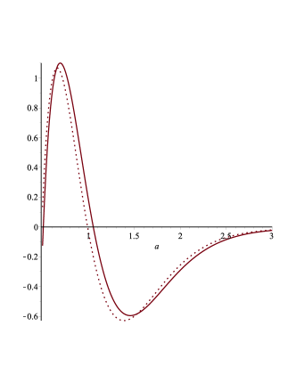
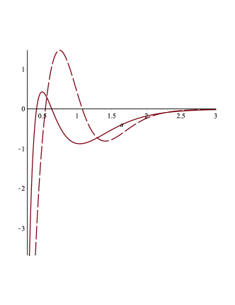
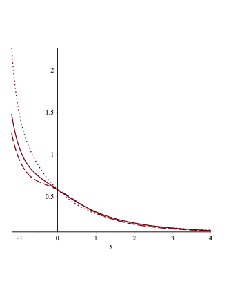
We note that $\ddot{a}>0$ (and thus $\tilde{q}>0$ ) corresponds to an accelerated stage. For $\gamma=1$ , we plot $\tilde{q}$ for different values of $w_{a}$ , $w_{0}$ , and the central value of $\Omega_{m}$ , and observe that at $a_{0}=1$ (the present stage), acceleration occurs only in certain cases (see Fig. 1 and Fig. 2).

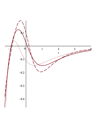
An important parameter related to the acceleration of the Universe is the deceleration parameter $q$ Visser . This parameter is defined as a criterion to determine the accelerated stages of the Universe. In our case, $q$ is expressed as follows

	$\displaystyle q$	$\displaystyle\equiv$	$\displaystyle-\frac{\ddot{a}a}{\dot{a}^{2}},$		(61)
		$\displaystyle=$	$\displaystyle\frac{1}{2}\left[1+\frac{3\Omega_{m}(\gamma-1)a^{-3\gamma}+3(1-\Omega_{m})(w_{0}+w_{a}(1-a))a^{-3(1+w_{o}+w_{a})}e^{3w_{a}(a-1)}}{\Omega_{m}a^{-3\gamma}+(1-\Omega_{m})a^{-3(1+w_{o}+w_{a})}e^{3w_{a}(a-1)}}\right].$		(62)

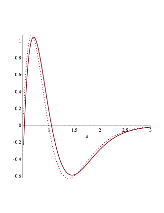
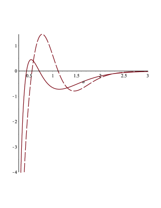
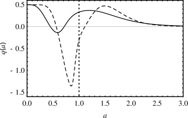
A negative value of $q$ clearly indicates an accelerated stage. Therefore, it is useful to plot $q(a)$ for the case where $\gamma=1$ , which is given by

q(a)_{\gamma=1}=\frac{1}{2}\left[1+3\frac{(1-\Omega_{m})(w_{0}+w_{a}(1-a))a^{-3(w_{0}+w_{a})}e^{3w_{a}(a-1)}}{\Omega_{m}+(1-\Omega_{m})a^{-3(w_{0}+w_{a})}e^{3w_{a}(a-1)}}\right].

(63)

We observe that at $a_{0}=1$ , the parameter is positive for the central values of $w_{0}$ , $w_{a}$ , and $\Omega_{m}$ , suggesting that the Universe is not currently in an accelerated stage (see Fig. 3 and Fig. 4).

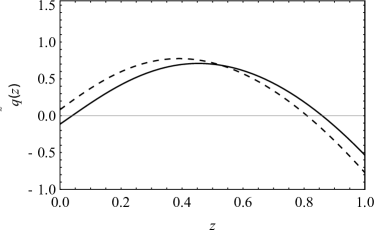
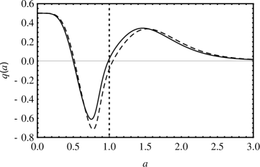
Notice that $\tilde{q}(a)$ and $q(a)$ are different functions, but qualitatively give the same information on the acceleration. To explore the global behaviour across different scale factors $a$ , we have plotted $\tilde{q}=3\ddot{a}/(4\pi G\rho_{crit})$ as a function of $a$ in Fig. 1 and Fig. 2. It is clear that at $a=1$ , the acceleration is not always positive. More importantly, the behaviour of the acceleration stands in stark contrast to the $\Lambda$ CDM Universe. Indeed, in terms of acceleration, the two Universes differ significantly from each other.

In particular, from Figs. 1 and 2 it is evident that the regions of positive acceleration change while allowing different values permitted by the fit. Here a small comment about the choices of parameters is due. According to Fig.6 of reference DESI the values of $w_{0}$ and $w_{a}$ are correlated. This makes the choice of $w_{a}=-1.31$ and $w_{0}=-0.16$ as well as $w_{a}=-2.79$ and $w_{0}=-0.76$ slightly outside the contours, but it is done here on purpose to display how the revelant physical quantities change if we move in this direction of the parameter space. This comment refers also to the rest of the paper.

Whereas for the central values of the fit the positive acceleration happens roughly in the region $0.5<a<1$ , choosing $w_{a}=-1.31$ and $w_{0}=-0.16$ makes this range shorter.

An important parameter in astrophysics is the cosmological redshift $z$ related to the scale factor by $a=(1+z)^{-1}$ . The behavior of $\tilde{q}$ with $z$ is shown in Fig. 3. To compare these results with the corresponding ones of $\Lambda$ CDM model we can readily infer that

\tilde{q}_{\Lambda CDM}=-[\Omega_{m}a^{-3}-2\Omega_{\Lambda}]=2\Omega_{\Lambda}-\Omega-m(1+z)^{3}

(64)

Using Planck data this tells us that in the $\Lambda$ CDM model the Universe is always accelerated provided $a>0.613$ ( $z<0.63$ ). In the Quntessence-DESI model the Universe is mostly accelerated in the past roughly below $a<1$ and remains positive up to $z\simeq 0.85$ , i.e., up to a higher value of $z$ as compared to the $\Lambda$ CDM model. This fact could eventually be used to discriminate the models.

The parameter $q$ has been plotted in Fig. 4. At $a=a_{0}=1$ , the current value of $q$ has been determined in Cosmographic . Some of the values for this parameter are model-independent and we list them in Table 4. For the DESI Quintessence model, we can also calculate the current value of $q_{0}$ , as follows

q(a=1)=\frac{1}{2}\left[1+3w_{0}(1-\Omega_{m})\right],

(65)

which, for the central values $w_{0}=-0.45$ and $\Omega_{m}=0.295$ , yields $(q_{0})_{\rm DESI}=0.024125$ , while for $\Omega_{m}=0.344$ it yields $(q_{0})_{\rm DESI}=0.0572$ .

Hubble data
Model	$H_{exp}$	GP	GA	$\Lambda$ CDM
$q_{0}$	-1.070 $\pm$ 0.093	-0.856 $\pm$ 0.111	-0.545 $\pm$ 0.107	-0.645 $\pm$ 0.023
Pantheon data
Model	$H_{exp}$	GP	GA	$\Lambda$ CDM
$q_{0}$	-0.616 $\pm$ 0.105	-0.558 $\pm$ 0.040	-0.466 $\pm$ 0.244	-0.572 $\pm$ 0.018

Table 4: Values of the present deceleration parameter

q_{0}

Cosmographic .

It is clear that the value of the deceleration parameter for DESI differs from the corresponding values in Table 4.

III.3 Solution for the scale factor

In this section, we will explore both numerical and analytical solutions for the scale factor.

III.3.1 Numerical solution for the scale factor $a$

By introducing the Hubble time $s=H_{0}t$ , we can rewrite (31) as

\left(\frac{a^{{}^{\prime}}}{a}\right)=\frac{8\pi G}{3H_{0}^{2}}(\rho_{\phi}+\rho),

(66)

where the prime denotes differentiation with respect to $s$ . Moreover, considering that $\Omega_{m}=\rho_{0}/\rho_{crit}$ and $\rho_{\phi,0}=\rho_{crit}-\rho_{0}$ , along with (35) and (44), we arrive at the following initial value problem

\frac{a^{{}^{\prime}}}{a}=\sqrt{\frac{\Omega_{m}}{3a^{3}}+\frac{1-\Omega_{m}}{3}a^{-3(1+w_{0}+w_{a})}e^{3w_{a}(a-1)}},\quad a(0)=1.

(67)

We solved the equation above using Maple and the Runge-Kutta-Fehlberg method. Figure 5 shows the behaviour of the scale factor for different parameter choices entering in equation (67). The solutions represented by the solid, dotted and dashed lines cannot be further computed beyond $a=-1.65199$ , $a=-1.51944$ , and $a=-1.75824$ , respectively. The case $\omega_{m}=0.295$ is shown in Figure 6. The solutions corresponding to the solid, dotted and dashed lines cannot be further computed beyond $a=-1.66141$ , $a=-1.50890$ , and $a=-1.73886$ , respectively.

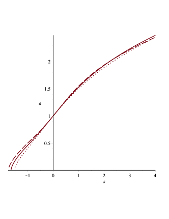
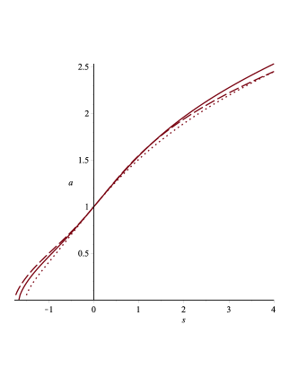
We have plotted the solution for $\Omega_{m}=0.285$ ((see Fig. 5) and $\Omega_{m}=0.295$ (see Fig. 6), even though the differences between the two cases are minimal. However, it is important to explicitly observe this fact. A careful inspection of these solutions reveals that they exhibit two inflection points, consistent with our discussion on acceleration. The curve begins concave, then becomes convex, and finally turns concave again. This behaviour contrasts with the $\Lambda$ CDM solution in (17), which is characterized by a shifted $sinh$ function with a single inflection point. We take this opportunity to revisit the acceleration’s independence from the Hubble time $s$ . This is indeed confirmed, as shown in Fig. 8. Both this figure and Fig. 7 were generated from the numerical solution for $a(s)$ using Maple18. In Fig. 7, we have plotted the Hubble parameter $H$ versus the Hubble time $s$ . Interestingly, for different parameter choices in the DESI fit, $H$ remains insensitive for $S>0$ , but shows significant differences in the range $s<0$ . It is in this region where the behaviour diverges considerably from the solution (16) of the cosmological constant model.

In the following, we will construct approximate analytical solutions for small and large values of $a$ , as well as for $a$ around $1$ .

III.3.2 Solution for $a$ around 1

Let $\gamma=1$ . We first rewrite (47) as follows

\frac{da}{dt}=\pm\sqrt{\frac{A+Ba^{\alpha}e^{\beta(a-1)}}{a}}

(68)

where

A=\frac{8}{3}\pi G\rho_{0},\quad B=\frac{8}{3}\pi G\rho_{\phi,0},\quad\alpha=-3(w_{0}+w_{a})>0,\quad\beta=3w_{a}<0,

(69)

and with the initial condition $a(0)=1$ . Using Maple, we obtain the following series solution in a neighbourhood of $a(0)=1$

	$\displaystyle a(t)$	$\displaystyle=$	$\displaystyle 1\pm\sqrt{A+B}t-\frac{1}{4}\left[A+(1+3w_{0})B\right]t^{2}$		(70)
			$\displaystyle\pm\frac{\sqrt{A+B}}{12}\left[2(A+B)+3B(3w_{0}^{2}+3w_{0}+w_{a})\right]t^{3}+\mathcal{O}(t^{4}).$		(70)

Differentiating the above expression twice with respect to the time variable, we find that around $a(0)=1$ the acceleration behaves as

\ddot{a}(t)=-\frac{1}{2}\left[A+(1+3w_{0})B\right]\pm\frac{\sqrt{A+B}}{2}\left[2(A+B)+3B(3w_{0}^{2}+3w_{0}+w_{a})\right]t+\mathcal{O}(t^{2}).

(71)

Note that the requirement $\ddot{a}(0)>0$ implies that the term $A+(1+3w_{0})B$ must be negative. It is straightforward to check that this inequality is equivalent to (55).

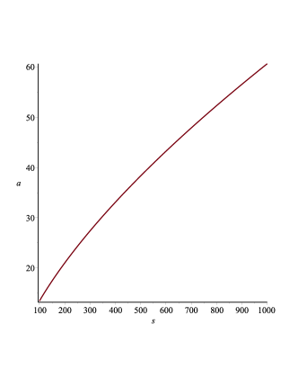
III.3.3 Solution for large $a$

Let $\gamma=1$ and rewrite the argument of the square root in (68) as follows

	$\displaystyle\frac{A+Ba^{\alpha}e^{\beta(a-1)}}{a}$	$\displaystyle\approx$	$\displaystyle\frac{A}{a}+Ba^{\alpha-1}e^{-\|\beta\|a},$		(72)
		$\displaystyle=$	$\displaystyle\frac{8}{3}\pi G\left(\frac{\rho_{0}}{a}+\rho_{\phi,0}a^{\alpha-1}e^{-\|\beta\|a}\right).$		(73)

According to the CMB data, the term $\alpha-1$ is positive and can take on values in the range $[3.11,9.35]$ . Furthermore, $\beta$ is negative, indicating an exponential decay as $a$ increases. Substituting $\rho_{0}=\Omega_{m}\rho_{crit}$ and $\rho_{\phi,0}=(1-\Omega_{m})\rho_{crit}$ gives

\frac{A+Ba^{\alpha}e^{\beta(a-1)}}{a}\approx\frac{8}{3a}\pi G\rho_{crit}\left[\Omega_{m}+(1-\Omega_{m})a^{\alpha}e^{-|\beta|a}\right].

(74)

Thus, in the regime where $a\gg 1$ , the right-hand side of equation (47) can be expressed as

\frac{A+Ba^{\alpha}e^{\beta(a-1)}}{a}\approx\frac{8}{3a}\pi G\rho_{crit}\Omega_{m}.

(75)

As a result, $a$ asymptotically satisfies the following equation

\frac{da_{\infty}}{dt}=\pm\sqrt{\frac{K}{a_{\infty}}},\quad K=\frac{8}{3}\pi G\rho_{crit}\Omega_{m}.

(76)

Integrating this equation yields

\frac{2}{3}a_{\infty}^{3/2}=\pm\sqrt{K}t+C,

(77)

where $C$ is an arbitrary integration constant that can be neglected when $t\gg 1$ . This leads to the asymptotic solution

a_{\infty}(t)\approx\sqrt[3]{12\pi G\rho_{crit}\Omega_{m}}t^{2/3}.

(78)

As Dark Energy diminishes and eventually vanishes at large times, the model transitions to a simple cosmology with $k=0$ and $\Lambda=0$ , preventing any collapse Nar . This behaviour is also illustrated in Fig. 9.

III.3.4 Solution for small $a$

In the scenario of small $a$ , we can assume we are in the radiation epoch, where $\gamma=4/3$ . First, we rewrite (47) as follows

\frac{da}{dt}=\pm\frac{\sqrt{A+Ba^{1+\alpha}e^{\beta(a-1)}}}{a}

(79)

with $A$ , $B$ , $\alpha$ and $\beta$ defined as in (68). Given that $1+\alpha$ is positive, as confirmed by the CMB data, we can Taylor expand the numerator in (79), leading to the following simplified differential equation

\frac{da_{0}}{dt}=\pm\frac{\sqrt{A}}{a_{0}}.

(80)

The corresponding solution is straightforward to obtain and is given by

a_{0}(t)=\sqrt{2\left(C\pm\sqrt{\frac{8}{3}\pi G\rho_{crit}\Omega_{m}}t\right)},

(81)

where $C$ is an integration constant chosen such that $a(T)=0$ for some $T<0$ .

III.4 Lifetime of the Universe

The bounds on the lifetime of the Universe serves as a powerful tool for evaluating the validity of cosmological models our , as the Universe cannot be younger than the objects it contains. Of particular relevance are the lower bounds on the Universe’s age, especially when considering some of the oldest galaxies and stars detected in our observable Universe. For the oldest galaxies, the lower limit is approximately $12.5$ Gyr Age1 , Age2 , while some of the oldest stars have been estimated to be even older, with a lower limit ranging between $13.2$ and $13.53$ Gyr Age3 , Age4 , Age5 . These ages have been determined using chemodynamical and Population III models, and they appear to be influenced by data from the CMB.

In the DESI Quintessence model, the lifetime of the Universe can be determined by

T_{\rm Univ}=\left|\int_{a=a_{0}=1}^{a=0}\frac{da}{a\sqrt{f(a)}}\right|.

(82)

Considering that $\rho_{crit}=3H_{0}^{2}/8\pi G$ , and introducing the dimensionless quantity $\Omega_{m}=\rho_{0}/\rho_{crit}$ with $\rho_{\phi,0}=\rho_{crit}-\rho_{0}$ , we can rewrite the integral as

T_{Univ}H_{0}=\left|\int_{0}^{1}\frac{da}{a\sqrt{\Omega_{m}a^{-3}+(1-\Omega_{m})a^{-3(1+w_{0}+w_{a})}e^{3w_{a}(a-1)}}}\right|.

(83)

The numerical values corresponding to this equation, using different allowed values for $w_{a}$ and $w_{0}$ are presented in the Tables V-VIII. Table V corresponds to the actual DESI fit with variable equation of state. The other tables show the differences when we change the Hubble constant and/or the matter density.

Table 5: Lifetime of the Universe in DESI Quintessence model with

\Omega_{m}=0.344

$H_{0}=(64.7^{+2.2}_{-3.3})$ Km s^-1 Mpc^-1		$\frac{1}{H_{0}}$ =(15.11 ${}^{+0.8}_{-1.2}$ ) Gyr
$w_{a}$	$w_{0}$	$T_{\rm Univ}\cdot H_{0}$	$T_{\rm Univ}$ (Gyr)
-1.79	-0.45	0.90652	13.70
-1.79-1.0	-0.45-0.21	0.9471	14.31
-1.79+0.48	-0.45+0.34	0.8346	12.61

The age of the oldest stars of $13.53$ Gyr comes very close to the $13.7$ Gyr estimated in Table 5. It all depends if stars could have formed $170$ million years after the Big Bang. We also notice that the Hubble parameter corresponding to the fit used in the Table 5 has a relative big error bar. This means that some allowed values of Hubble parameter will lead to a smaller lifetime. For instance, using $H_{0}^{-1}=(15.11-0.6)$ Gyr we arrive at lifetime of the universe of $13.15$ Gyr which is again smaller than the age of the oldest stars.

Table 6: Lifetime of the Universe in DESI Quintessence model with

\Omega_{m}=0.285

$H_{0}=(68.3\pm 1.1)$ km s^-1 Mpc^-1		$\frac{1}{H_{0}}$ =(14.316 $\pm$ 0.2) Gyr
$w_{a}$	$w_{0}$	$T_{\rm Univ}\cdot H_{0}$	$T_{\rm Univ}$ (Gyr)
-1.79	-0.45	0.95378	13.65
-1.79-1	-0.45-0.21	1.00498	14.39
-1.79+0.48	-0.45+0.34	0.86531	12.39

Table 7: Lifetime of the Universe in DESI Quintessence model with

\Omega_{m}=0.295

$H_{0}=(68.3\pm 1.1)$ Km s^-1 Mpc^-1		$\frac{1}{H_{0}}$ =(14.316 $\pm$ 0.2) Gyr
$w_{a}$	$w_{0}$	$T_{\rm Univ}\cdot H_{0}$	$T_{\rm Univ}$ (Gyr)
-1.79	-0.45	0.94499	13.53
-1.79-1.0	-0.45-0.21	0.99417	14.23
-1.79+0.48	-0.45+0.34	0.85966	12.31

Table 8: Lifetime of the Universe in DESI Quintessence model with

\Omega_{m}=0.344

$H_{0}=(68.3\pm 1.1)$ Km s^-1 Mpc^-1		$\frac{1}{H_{0}}$ =(14.316 $\pm$ 0.2) Gyr
$w_{a}$	$w_{0}$	$T_{\rm Univ}\cdot H_{0}$	$T_{\rm Univ}$ (Gyr)
-1.79	-0.45	0.90652	12.98
-1.79-1.0	-0.45-0.21	0.9471	13.56
-1.79+0.48	-0.45+0.34	0.8346	11.95

However, it is also possible to consider the reverse conclusion. If the lifetime of a new cosmological model is smaller than the lifetime of the oldest stars we could equally conclude that such estimates of the ages of the oldest stars may not be accurate as the latter are model dependent. A more model independent approach is presented below.

Returning to the tables in Section II, the Tables 2 and 3 present the results for the lifetime of the universe for one of the DESI fits with a constant parameter $w$ in the equation of state. Notably, some of the calculated lifetimes (especially those in Table 2) within the $\Lambda$ CDM model face some challenges if we accept the current estimates for the ages of the oldest stars.

Galaxies observed at a high cosmological redshift $z$ Age1 , CosmicDawn offer also a good test of the validity of a given model. In this case the time needed to reach the observer $\Delta t$ should always be smaller then the lifetime of the universe. One needs a relation between the cosmological redshift $z$ and $\Delta t$ which is readily obtained from

a=\frac{1}{1+z},

(84)

and the definition of the Hubble function

H=\frac{1}{a}\frac{da}{dt}=(1+z)\frac{da}{dz}\frac{dz}{dt}

(85)

This allows us to write

dt=-\frac{1}{H_{0}}\frac{dz}{(1+z)E(z)^{1/2}}

(86)

where we used

\left(\frac{H(z)}{H_{0}}\right)^{2}\equiv E(z)

(87)

Here $H(z)$ follows from the Friedmann equations. For instance, in the $\Lambda$ CDM model we have

\Delta t=\frac{1}{H_{0}}\int_{0}^{z_{e}}\frac{dz}{(1+z)\sqrt{\Omega_{m}(z+1)^{3}+\Omega_{\Lambda}}}=\frac{1}{H_{0}}\left[-\frac{2}{3\sqrt{\Omega_{\Lambda}}}\coth^{-1}\left(\sqrt{\frac{\Omega_{m}(1+z)^{3}+\Omega_{\Lambda}}{\Omega_{\Lambda}}}\right)\right]\Bigg{|}_{z=0}^{z=z_{e}}

(88)

whereas the Quintessence model would give rise to

\Delta t=\frac{1}{H_{0}}\int_{0}^{z_{e}}\frac{dz}{(1+z)\left[(1-\Omega_{m})(1+z)^{3(1+w_{0}+w_{a})}e^{-3w_{a}\frac{z}{z+1}}+\Omega_{m}(z+1)^{3}\right]^{1/2}}

(89)

The lifetime of the universe is obtained in both formulas by taking $z_{e}\to\infty$ . The values of $\Delta t$ for several relevant redshifts $z$ in both $\Lambda$ CDM and Quintessence models are given in Tables 9 and 10. The evidence of the luminous objects at very high redshift we have taken from Laursen , Yan . For $z=16-20$ we have used Fig.6 in Laursen . The value $z=24.7$ is mentioned in Yan , but as stated there is subject to the interpretation of the templates. At the same time, this very high redshift has prompted the author to point out that the next challenge is to find objects beyond $z=20$ . The values of the time span $\Delta t$ needed to reach us are displayed in tables IX. and X. In general, there is a tension between the lifetime of the Universe. If we change the values of $w_{a}$ and $w_{0}$ and push them to the border of the allowed parameter space it is possible to obtain a higher lifetime in the Quintessence-DESI model (see table V). In both models we face the problem of the so-called “impossible early galaxy” formation Steinhardt1 . This could be due to the cosmological model (a too short lifetime) or due to the interpretation of the images Steinhardt2 . A third possibility is some unknown physics at the early epoch of the Universe.

Table 9: Time needed to reach an observer

\Delta t

for high redshifts in different

\Lambda

CDM fits.

$\Lambda$ CDM Fit	$H_{0}$ (Km s^-1 Mpc^-1)	$\Omega_{m}$	$\Omega_{\Lambda}$	$z_{e}$	$\Delta tH_{0}$	$\Delta t$ (Gyrs)
Planck	67.36 $\pm$ 0.54	0.3153	0.6847	12	0.9254	13.43
				$\quad 13\quad$	0.9281	13.47
				14	0.9303	13.50
				$16$	0.9338	13.55
				$20$	0.9384	13.62
				$24.7$	0.9416	13.67
				$\infty$	0.95073	13.80
DESI	67.97 $\pm$ 0.38	0.3069	0.6931	12	0.9323	13.41
				13	0.935	13.45
				14	0.9373	13.48
				$16$	0.9408	13.53
				$20$	0.9454	13.60
				$24.7$	0.9487	13.65
				$\infty$	0.958	13.78
DESI+CMB+BAO	68.3 $\pm$ 1.1	0.349	0.651	12	0.8996	12.88
				13	0.9022	12.92
				14	0.9043	12.95
				$16$	0.9076	12.99
				$20$	0.9119	13.06
				$24.7$	0.91504	13.10
				$\infty$	0.9237	13.22

Table 10: Time needed to reach an observer

\Delta t

for high redshifts in different non-constant equation of state fits (

w_{0}w_{a}\Lambda

CDM).

$\quad w_{0}w_{a}$ $\Lambda$ CDM Fit	$H_{0}$ (Km s^-1 Mpc^-1)	$\quad\Omega_{m}\quad$	$\quad\Omega_{\Lambda}\quad$	$z_{e}$	$\Delta tH_{0}$	$\Delta t$ (Gyrs)
DESI	68.3 $\pm$ 1.1	0.344	0.656	12	0.8823	12.63
				$\quad 13\quad$	0.8848	12.67
				14	0.8870	12.70
				$16$	0.8903	12.75
				$20$	0.8947	12.81
				$24.7$	0.8978	12.85
				$\infty$	0.9065	12.98
DESI + CMB	64.7 ${}^{+2.2}_{-3.3}$	0.344	0.656	12	0.8823	13.33
				13	0.8848	13.37
				14	0.8870	13.40
				$16$	0.8903	13.46
				$20$	0.8947	13.52
				$24.7$	0.8978	13.57
				$\infty$	0.9065	13.70

IV Conclusions

The recent fits of cosmological parameters by the DESI collaboration DESI , if confirmed, have the potential to shift our cosmological model from $\Lambda$ CDM to one that allows for a variable (scale factor-dependent) parameter $w(a)$ in the equation of state. This model would most likely correspond to a quintessence model or $f(R)$ gravity. Given the significance of such a paradigm shift in cosmology, we have conducted various consistency checks. They include an examination of the acceleration of the expansion, which has dominated cosmology over the past few decades, with observational evidence pointing to a positive acceleration and the theoretical efforts to explain it. The DESI fit in the Quintessence parametrization shows a positive acceleration, i.e. $\ddot{a}>0$ , roughly for $0<z<0.85$ . But the decelaration parameter at the present epoch does not agree with model independent estimates. Nevertheless one could use the fact that in the DESI-Quintessence model the acceleration lasts longer into the past as a discriminating point while observing distant supernovae. The $\Lambda$ CDM model has a positive acceleration in the future ( $a>1$ ) where the DESI-Quintessence model shows here a negative value.

Another crucial cosmological parameter is the lifetime of the Universe. Accepting the existence of old stars and galaxies, any viable model should eventually be properly constrained by these values. The DESI-Quintessence model satisfies this requirement only for some values of the allowed parameter space. This is true for the time dependent fit of the equation of state as well as for constant one which would correspond to the $\Lambda$ CDM model. The problem of luminous objects at a high cosmological redshift reveals a problem for both models which can be framed as a “too early structure formation” after the Big Bang Steinhardt1 , Laursen , Steinhardt3 . Since the parameter space of the DESI fit allows also bigger lifetimes of the Universe we see this as an opportunity for the time dependent DESI if, using an adequate time scale contraint from structure formation, we allow only values leading to a bigger lifetime.

A remark is deemed necessary here to clarify the DESI-Quintessence terminology. As mentioned in Section II, it is sufficient to consider the phenomenological equations (21) and (22), which might encompass a broader class of models-though they would likely be indistinguishable from the Quintessence model, as the Friedmann equations are identical. Finally, our study is supplemented by numerical and approximate analytical solutions for the scale factor.

References

[1] N. S. Hetherington (ed), Encyclopedia of cosmology, Garland Publishing, New York (1993); J. North, Cosmology: An illustrated history of Astronomy and Cosmology, The University of Chicago Press (2008).
[2] S. Weinberg, Gravitation and Cosmology: Principles and Applications of the General Theory of Relativity, Wiley & Sons, New York (1972).
[3] S. Weinberg, The cosmological constant problem, Rev. Mod. Phys. 61, 1 (1989); T. Padmanabhan, Cosmological Constant-the Weight of the Vacuum, Phys. Rept. 380, 235 (2003).
[4] G. Bertone, Particle Dark Matter: Observations, Models and Searches, Cambridge University Press, Cambridge (2013); N. C. M. Martens and M. King, Doing More with Less: Dark Matter and Modified Gravity in N. Mills Boyd, S. de Baerdemaeker, K. Heng and V. Matarese (eds.), Philosophy of Astrophysics: Stars, Simulations and the Struggle to Determine What is Out There, Springer (2023).
[5] T. P. Sotiriou and V. Faraoni, $f(R)$ theories of gravity, Rev. Mod. Phys. 82, 451 (2010).
[6] A. De Felice and S. Tsujikawa, $f(R)$ theories, Living Rev. Rel. 13: 3 (2010).
[7] G. J. Olmo Palatini Approach to Modified Gravity: $f(R)$ Theories and Beyond, Int. J. Mod. Phys. D 20, 413 (2011).
[8] R. Myrzakulov, FRW cosmology in $F(R,T)$ gravity, Eur. Phys. J. C 72, 2203 (2012).
[9] J. Wu, G. Li, T. Harko and S. Liang, Palatini formulation of $f(R,T)$ gravity theory, and its cosmological implications, Eur. Phys. J. C 78, 430 (2018).
[10] N. Katirci and M. Kavuk, $f(R,T_{\mu\nu}T^{\mu\nu}$ gravity and Cardassian-like expansion as one of its consequences, Eur. Phys. J. Plus 129, 163 (2014).
[11] M. Roshan and F. Shojai, Energy-Momentum Squared Gravity, Phys. Rev. D 94, 044002 (2016).
[12] C. V. R. Board and J.D. Barrow, Cosmological Models in Energy-Momentum-Squared Gravity, Phys. Rev. D 96, 123517 (2017).
[13] Y. Cai, S. Capozziello, M. De Laurentis and E. N. Saridakis, $f(T)$ teleparallel gravity and cosmology, Rept. Prog. Phys. 79, 106901 (2016).
[14] R. Yang, New types of $f(T)$ gravity, Eur. Phys. J. C 71, 1797 (2011).
[15] S. Capozziello, V. F. Cardone, H. Farajollahi and A. Ravanpak, Cosmography in $f(T)$ -gravity, Phys. Rev. D 84, 043527 (2011).
[16] L. Heisenberg, Review on $f(Q)$ Gravity, Phys. Rept. 1066, 1 (2024).
[17] W. Khyllep, J. Dutta, E. N. Saridakis and K. Yesmakhanova, Cosmology in $f(Q)$ gravity: A unified dynamical system analysis at background and perturbation levels, Phys. Rev. D 107, 044022 (2023).
[18] K. Koussour, K. El Bourakadi, S.H. Shekh, S.K.J. Pacif and M. Bennai, Late-time acceleration in $f(Q)$ gravity: Analysis and constraints in an anisotropic background, Ann. Physics, 445, 169092 (2022).
[19] J. B. Jimenez, L. Heisenberg, T. Koivisto, and S. Pekar, Cosmology in $f(Q)$ geometry, Phys. Rev. D 101, 103507 (2020).
[20] Y. X., Guangjie Li, T. Harko and Shi-Dong Liang, $f(Q,T)$ gravity, Eur. Phys. J. C 79, 708 (2019).
[21] M. Shiravand, S. Fakhry, and M. Farhoud, Cosmological Inflation in $f(Q,T)$ Gravity, Physics of the Dark Universe 37, 101106 (2022).
[22] Y. Xu, T. Harko, S. Shahidi and S. Liang, Weyl type $f(Q,T)$ gravity, and its cosmological implications, Eur. Phys. J. C 80, 449 (2020).
[23] S. Bahamonde et al., Teleparallel Gravity: From Theory to Cosmology, Rep. Prog. Phys. 86, 026901 (2023).
[24] Yu. N. Obukhov and J. G. Pereira, Metric-affine approach to teleparallel gravity, Phys. Rev. D 67, 044016 (2003).
[25] L. Heisenberg, M. Hohmann and S. Kuhn, Homogeneous and isotropic cosmology in general teleparallel gravity, Eur. Phys. J. C 83, 315 (2023).
[26] S. Nojiri, S.D. Odintsov and V.K. Oikonomou, Modified Gravity Theories on a Nutshell: Inflation, Bounce and Late-time Evolution, Phys. Rept. 692, 1 (2017).
[27] F. Payadeh, and M. Fathi, $R^{2}$ Theory of Gravity, J. Phys. Conf. Ser. 442, 012053 (2013).
[28] E. V. Arbuzova, A. D. Dolgov and L. Reverberi, Cosmological evolution in $R^{2}$ gravity, JCAP 02, 049 (2012).
[29] T. Harko, F. S.N. Lobo, S. Nojiri and S. D. Odintsov, $f(R,T)$ gravity, Phys. Rev. D 84, 024020 (2011).
[30] T. Harko, and F.S.N. Lobo, $f(R,L_{m})$ gravity, Eur. Phys. J. C. 70, 373 (2010).
[31] L. Verde, T. Treu, and A.G. Riess, Tensions between the Early and the Late Universe, Nat. Astron. 3, 891 (2019).
[32] E. Di Valentino et al., In the Realm of Hubble Tension-a Review of Solutions, Class. Quantum Grav. 38, 153001 (2021); W.D. Kenworthy, D. Scolnic and A. Riess, The Local Perspective on the Hubble Tension: Local Structure Does Not Impact Measurement of the Hubble Constant, ApJ 875, 145 (2019).
[33] A. G. Adame et al., DESI 2024 VI: Cosmological Constraints from the Measurements of Baryon Acoustic Oscillations, arXiv:2404.03002 [astro-ph.CO].
[34] Y. Tada and T. Terada, Quintessential interpretation of the evolving dark energy in light of DESI, Phys. Rev. D 109, L121305 (2024).
[35] S. Perlmutter et al., Measurements of Omega and Lambda from 42 High-Redshift Supernovae, ApJ 517 565, (1999).
[36] A.G. Riess et al., Observational Evidence from Supernovae for an Accelerating Universe and a Cosmological Constant, AJ 116 1009, (1998).
[37] S. Bravo Medina, Marek Nowakowski, R. V. Lobato and D. Batic, Cosmologies in f(R, $L_{m}$ ) with non-minmal coupling between geometry and matter, Phys. Scr. 99, 065050 (2024).
[38] H. P. Robertson, Kinematics and World-Structure, ApJ 82, 284 (1935); A.G. Walker, On Milne’s Theory of World-Structure, Proc. Lond. Math. Soc., 42, 90 (1936).
[39] J. Frieman, M. Turner and D. Huterer, Dark Energy and the Accelerating Universe, Ann. Rev. Astron. Astrophys. 46,385 (2008).
[40] E. Kolb and M. Turner, The Early Universe, Westview Press (1990).
[41] R. Aldrovandi, R. R. Cuzinatto and L. G. Medeiros, Analytic solutions for the $\Lambda$ -FRW Model, Found. Phys. 36, 1736 (2006).
[42] A. Mehrabi, and M. Rezaei, Cosmographic parameters in model-independent approaches, ApJ 923, 274, (2021).
[43] E. V. Linder, Exploring the expansion history of the universe, Phys. Rev. Lett. 90, 091301 (2003).
[44] M. Chevallier and D. Polarski, Accelerating universes with scaling dark matter, Int. J. Mod. Phys. D 10, 213 (2001).
[45] N. Aghanim et al. Planck 2018 results, A& A 641, A6 (2020).
[46] S. Tsujikawa, Quintessence: A Review, Class. Quant. Grav. 30, 214003, (2013).
[47] E. Di Pietro and J. Demaret, A constant equation of state for quintessence?, Int. J. Mod. Phys. D 10, 231 (2001).
[48] T.P. Sotiriou and V. Faraoni, $f(R)$ Theories of Gravity, Rev. Mod. Phys. 82,451 (2010).
[49] A.A. Starobinsky, A new type of isotropic cosmological models without singularity, Phys. Rev. B 91, 99 (1980).
[50] Y. Shtanov, On the Conformal Frames in f(R) Gravity, Universe 8, 69 (2022).
[51] D. Mukherjee, H.K. Jassal and K. Lochan, $f(R)$ dual theories of quintessence: expansion–collapse duality, JCAP 12, 016 (2021).
[52] M. Visser, Jerk, snap and the cosmological equation of state, Class. Quant. Grav. 21, 2603 (2004).
[53] B. E. Robertson et al., Identification and properties of intense star-forming galaxies at redshifts $z>10$ , Nat. Astron. 7, 6 (2023); E. Curtis-Lake et al., Spectroscopic confirmation of four metal-poor galaxies at z = 10.3–13.2, Nat. Astron. 7, 622 (2023).
[54] C. Sneden, The age of the universe, Nature 409, 643 (2001); R Cayrel et al., Measurement of stellar age from uranium decay, Nature 409, 691 (2001).
[55] J. Tumlinson, Chemical Evolution in Hierarchical Models of Cosmic Structure II: The Formation of the Milky Way Stellar Halo and the Distribution of the Oldest Stars, Astrophys. J. 708, 1418, (2010).
[56] M.N. Ishigaki, N. Tominaga, C. Kobayashaki and K. Nomoto, Faint Population III supernovae as the origin of the most iron-poor stars, ApJL 792, L32 (2014).
[57] K.C. Schlaufman, I.B. Thompson and A.R. Casey, An Ultra Metal-poor Star Near the Hydrogen-burning Limit, ApJ 867, 98 (2018).
[58] J. V. Narlikar, Introduction to Cosmology, 3rd ed., Cambridge University Press (2002).
[59] S. Carniani et al., A shining cosmic dawn: spectroscopic confirmation of two luminous galaxies at $z\sim 14$ , arXiv:2405.18485 [astro-ph.GA].
[60] P. Laursen, Galaxy formation from a timescale perspective in J. Hesselbjerg Christensen, K. Richardson, O. Vallès Codina (eds) Multiplicity of Time Scales in Complex Systems. Mathematics Online First Collections Springer, 2023.
[61] H. Yan, Z. Ma and C. Ling, First Batch of $z\approx 11-20$ Candidate Objects Revealed by the James Webb Space Telescope Early Release Observations on SMACS 0723-73, ApJL 942, L9 (2023).
[62] C. L. Steinhardt, P. Capak, D. Masters and J. S. Speakle, The impossibly early galaxy problem, ApJ 824, 21 (2016).
[63] C. L. Steinhardt, V. Kokorev, V. Rusakiv, E. Garcia and A. Sneppen, Templates for Fitting Photometry of Ultra-High-Redshift Galaxies, arXiv:2208.07879.
[64] C. L. Steinhardt, V. Rusakov, T. H. Clark, A. Diaconu, J. Forbes , C. McPartland, A. Sneppenand J. Weaver The Earliest Stage of Galactic Star Formation, ApJL 949, L38 (2023).