The Vela Cloud: A Giant HI Anomaly in the NGC 3256 Group
Abstract
We present Australia Telescope Compact Array (ATCA) observations of a galaxy-sized intergalactic HI cloud (“the Vela Cloud”) in the NGC 3256 galaxy group. The group contains the prominent merging galaxy NGC 3256, which is surrounded by a number of HI fragments, the tidally disturbed galaxy NGC 3263, and several other peculiar galaxies. The Vela Cloud, with an HI mass of 3-5 , resides southeast of NGC 3256 and west of NGC 3263, within an area of 9′ 16′ (100 kpc 175 kpc for an adopted distance of 38 Mpc). In our ATCA data the Vela Cloud appears as 3 diffuse components and contains 4 density enhancements. The Vela Cloud’s properties, together with its group environment, suggest that it has a tidal origin. Each density enhancement contains of HI gas which is sufficient material for the formation of globular cluster progenitors. However, if we represent the enhancements as Bonnor-Ebert spheres, then the pressure of the surrounding HI would need to increase by at least a factor of 6 in order to cause the collapse of an enhancement. Thus we do not expect them to form massive bound stellar systems like super star clusters or tidal dwarf galaxies. Since the HI density enhancements have some properties in common with High Velocity Clouds, we explore whether they may evolve to be identified with these starless clouds instead.
1 Introduction
1.1 Intergalactic clouds
The detection of intergalactic clouds, such as the one studied in this paper, can illuminate the progress of galaxy evolution. For example, one expects to find primordial HI building blocks of hierarchical galaxy construction unless galaxy formation was extremely efficient. However these are rarer than predicted by the current cosmological theories which build galaxies via the hierarchical merging of proto-galactic clouds embedded in dark-matter halos (e.g. Klypin et al. 1999). Studies of groups of galaxies reveal very few metal-poor and star-poor clouds (e.g. Zwaan 2001 and papers referenced therein; Pisano et al. 2004). Other HI detections include bona fide dwarf galaxies (e.g. Côté et al. 2000); HI envelopes enclosing superwinds (e.g. Ott et al. 2005); and outflows from disks due to supernovae or buoyantly rising bubbles (e.g. Irwin & Chaves (2003) and papers mentioned therein) or plumes potentially due to ram pressure (e.g. Oosterloo & van Gorkom 2005). A strongly accepted explanation for many HI clouds is that they are tidal extensions from galaxies and/or tidal dwarf galaxies (e.g. Duc et al. 2004; Hibbard et al. 2001a; Hibbard et al. 2001b; Koribalski et al. 2003; Koribalski & Dickey 2004; Koribalski 2004). Tidal origins are also proposed for HI companions to HII galaxies (Taylor et al. (1993, 1995, 1996), the compact HI companion to FCC 35 (Putman et al., 1998), and the extended companion to NGC 2442 called HIPASS J0731-69 (Ryder et al., 2001). Indeed the Leo Ring (Schneider et al., 1983) is associated with a group of galaxies and is likely to have a tidal origin (Bekki et al., 2005b).
A similar debate also exists about the origins of the Galactic High Velocity Clouds (HVCs). Since stars in HVC have not yet been detected, their distances from the Milky Way are difficult to determine. Recent studies indicate that they are within tens of kpc (Bland-Hawthorn et al 1998; Putman et al 2003; Wakker et al. 2008). HVCs could be nearby tidal debris similar to fragments of the Magellanic Stream (e.g. Westmeier & Koribalski 2008, Putman et al. 2003b) or material cooling and infalling from a primordial halo (e.g. Peek et al. 2006 although see Binney, Nipoti & Fraternali 2009). Another alternative is that they are material ejected from the disk of our Galaxy to a height of a few kpc which subsequently rains back down onto the plane as a Galactic fountain (e.g. Norman & Ikeuchi 1989; Ganguly et al. 2005).
In order to clarify the origins of HVCs, there are numerous studies of extra-planar HI associated with individual galaxies. Since the detected HI clouds are in the vicinity of the host galaxies the origins of these clouds are interpreted as either a galactic fountain (e.g. Fraternali & Binney 2008) or tidal debris (e.g. Westmeier et al. 2007) or possibly a condensation from a primordial halo (e.g. Rand & Benjamin 2008).
A survey for extra-galactic HVCs in groups of galaxies by Pisano et al. (e.g. 2004, 2007, and papers mentioned therein) have detected optical counterparts to HI clouds, suggesting they are dwarf galaxies. Also the proximity of the dwarfs to individual galaxies within each group seems to argue against in-fall from outside a group’s radius, making a cosmological origin unlikely. That is, we would expect primordial cold clouds to fall towards the group’s centre of mass rather than predominantly orbit individual galaxies. The on-going merger NGC 3256 also displays HI fragments in its vicinity (English et al., 2003). However since they appear to be starless, they may be analogous to HVCs.
1.2 The Vela Cloud in the NGC 3256 Group
The NGC 3256 Group and NGC 3263 Group are difficult to distinguish from each other spatially and the systemic velocities of their eponymous galaxies differ by less than 200 . Additionally two different group-finding algorithms applied to the same dataset do not find the same galaxies in each group (Fouque et al. 1992; Garcia 1993). Many researchers therefore consider at least 15 galaxies to be members of a single large group spread over roughly a few degrees (eg. Lípari et al. 2000; Mould et al. 1991). We adopt this latter perspective for the remainder of the paper and refer to the association of galaxies as the NGC 3256 Group.
The most spectacular HI feature in the NGC 3256 Group is a galaxy-sized intergalactic HI cloud (English, 1994), which we will refer to as “the Vela Cloud”. The structure, as projected on the sky, is not clearly associated with an individual galaxy but appears to be part of the group. A tidal origin for the cloud is suggested by the fact that most of the galaxies in this region are tidally disturbed. This fact can be seen from those members of the group that are present in the field of view of our Australia Telescope Compact Array (ATCA) HI data (Fig. 1). The cloud’s potential evolution is also interesting, and this paper explores whether parts of the cloud could be identified with HVCs at some point in their evolution.
The Vela Cloud was initially detected in an ATCA pointing towards NGC 3256 (English, 1994; English et al., 2003) and further studied with 3 pointings of the Parkes Telescope (English, 1994). In this paper we present additional ATCA data with a pointing centre towards NGC 3263, which confirms the Vela Cloud’s existence (Fig. 1). The Vela Cloud appears to be a cohesive structure, with 3 distinct diffuse gas sub-components, which we have labelled A, B, and C; see the schematic in Fig. 2. Four HI density enhancements are seen and an aim of this paper is to consider whether the internal pressure within these enhancements satisfies the conditions for initiating star formation.
Our radio and optical (broad band and Fabry-Perot) observations and reductions are described in § 2. § 3 only describes measurement methods and the uncertainties associated with these methods. The actual measurements of the cloud’s observed characteristics are detailed in section § 4. In § 5 we describe derived characteristics (such as the amount of HI mass in emission), explore the star-forming potential in the Vela Cloud (representing the enhancements as Bonnor-Ebert spheres), and consider the ultraviolet radiation field of NGC 3263 in relation to the Vela Cloud. Then in § 6 the cloud’s characteristics are contrasted with those of tidal debris, and other apparently isolated clouds, including HVCs. In § 7, we discuss the likely role of the group’s tidal field on the origin of the Vela Cloud and speculate on the cloud’s fate, asking whether its enhancements may evolve into HVCs. § 8 summarizes our study of this rare galaxy-sized intergalactic cloud.
2 Observations
2.1 Radio Observations and Reductions.
21-cm line data were acquired using the ATCA in 1995 and 1996. The target centre was right ascension = 10h29m04s and declination = -44°04′12″(J2000), close to NGC 3263. At 1406 MHz, with a bandwidth of 8 MHz, the observations spanned that galaxy’s systemic and rotation velocities and included several other galaxies in the NGC 3256 Group. Array configurations 375, 750A, 1.5B, 6C were used to acquire 12.5, 10.2, 11.6, 10.7 hours, respectively. The longest baseline corresponds to a spatial resolution of 7 arcsec while the primary beam is 33 arcmin. These 4 UV datasets were flagged and calibrated, using AIPS and the calibrators PKS 1934-638 (primary) and PKS 0823-500 (secondary), in the usual way. The continuum emission was fit using the line-free emission on either side of the HI signal and subtracted in the UV plane. After converting their frequency axes to optically defined heliocentric velocities, the datasets from the 4 array-configurations were combined.
For the subsequent Fourier transformation, deconvolution, and analysis we used the Miriad software package. We base our data analysis on a cube with the parameters listed in Table 1 and on subcubes which span smaller velocity ranges (see § 3). The characteristics of the cubes used to produce Fig. 1 and Fig. 3 are listed in those figure captions. Although radio continuum observations were also made at 1380 MHz, the intergalactic cloud was not detected.
Single-dish telescope data were acquired on Dec. 19 and 20, 1993 using the single-feed 20-cm receiver at the 64-m Parkes Telescope, a bandwidth of 32 MHz, and 2 polarizations of 1024 channels each. The effective channel width is 8.2 . Observations were acquired for 3 different target positions on the sky. For each position 2 scans were acquired on-target along with 2 reference scans off-target. Each scan was 10 minutes. The off-target scans were subtracted from the on-target data and also used for normalization of the spectra; the r.m.s. is 0.013 Jy per channel. We present one of the target positions ( = 10h28m277, = -44°09′25″(J2000)) in this paper. While this pointing is west of NGC 3263, the 15′ beam width encompasses some emission from this galaxy. Details, and profiles of the other pointings, are provided in English (1994).
2.2 Optical Observations and Reductions
On the night of 27-28 Feb 1995 we observed the Vela Cloud with the TAURUS imaging Fabry-Perot interferometer mounted at the f/8 Cassegrain focus of the AAT 3.9m. We attempted to detect the HI cloud in H and [NII]6583Å emission using the Fabry-Perot ‘staring’ method which reaches the faintest possible levels in diffuse line emission (Bland-Hawthorn et al., 1994). The conditions were mostly photometric and dark, with the moon rising at the end of the night. We used the University of Maryland etalon with a 41 m gap spacing and a coating finesse of 50 at H. The blocking filter, which was centred at 6641Å with a 17Å bandpass, had a peak transmission of 73%. The measured free spectral range was 54.3Å at H such that the blocking filter isolated only one order. We employed a TEK 10242 CCD with 0.594” pixels and a read noise of 2.3 electrons in XTRASLOW mode. The technique results in observations acquired in an annular region which was centred at = 10h28m302, = -44°08′51″(J2000). The integration times are listed in Table 2.
The images were bias subtracted, flatfielded and corrected for filter transmission profile using twilight and whitelight frames respectively. Stars within the field were located with daophot and subsequently subtracted. The four data frames were combined and co-added using minmax clipping under imcombine in IRAF; this procedure successfully removed all cosmic rays and point-like artefacts. The data were azimuthally binned and corrected for the angular dispersion as discussed in Bland-Hawthorn et al. (1998). The final spectrum is dominated by two OH sky-lines at 6627.6Å and 6634.2Å. No H or [NII] emission can be detected at the level of EM(H) 60 mR and EM([NII]) 30 mR (3). Note that at 104K, EM(H) = 30 mR is equivalent to a surface brightness of erg cm-2 s-1 arcsec-2.
Using the Double-beam Spectrograph at the Siding Spring Observatory 2.3m telescope, a spectrum (§ 4.2) was acquired at = 10h28m2577, = -44°16′175 (J2000), at the position of the HII emission-line galaxy WPV060. The wavelength range is 6400-6850 Å, allowing the acquisition of 5 emission lines: H, [NII], [SII]. Using the of the calibration arclamp lines gives an uncertainty for the systemic velocity of 6 . The instrumental profile is 4.8Å which corresponds to a velocity resolution of . The reductions were carried out in the usual way using IRAF. For the spectrum and its analysis see § 4.2.
3 21 cm Emission-line Measurement and Analysis Techniques
As described in § 1.2, the Vela Cloud appears in our ATCA data as 3 large diffuse components which we have labelled A, B, and C (Figure 2). This current section describes the techniques, including the uncertainties, used to measure the observed characteristics of these diffuse component clouds (§ 3.1) and the enhancements embedded in them (§ 3.2). The measurements themselves are presented in section § 4.
3.1 The Diffuse Emission in Components A, B, and C
For each diffuse cloud component sketched in Fig 2, the Full-Width-Half-Maximum (FWHM) value (§ 4.1) was determined from velocity profiles which were generated interactively using the Karma visualization package (Gooch, 1996). An uncertainty of 10-15% includes the difference between measuring smoothed and unsmoothed profiles and the variation produced by visually selecting slightly different sized rectangles to encompass the component.
Dimensions and integrated flux densities were measured from integrated intensity (i.e. zero moment) maps generated using moment in Miriad. All measurements were made on data corrected for the primary beam response; however in the case of integrated intensity maps, the primary beam correction was applied to each moment map. Using cloud component B, we compared this approach to constructing moment maps from primary beam corrected cubes. For these comparison maps, a smoothed mask cube was applied to a primary beam corrected cube and values above a 3 in the mask are retained and then a moment map was created from the resultant blanked cube. To create the mask cube, the primary beam corrected data were spatially smoothed using a Gaussian of 3 beam widths and Hanning smoothed in velocity using 3 channels (see Table 3). We note that the Vela Cloud is clearly evident in this mask cube. This second approach gave an integrated flux density for component B that was 14% higher than the value from the primary beam-corrected moment map approach. Since the primary beam-corrected moment map approach generates smaller values, which will produce conservative mass estimates, we list these for the integrated flux density, (in Jy km s-1), in Table 3 and in § 4.1. The difference between measuring the flux density using moment maps (in which weak features may be clipped) and summing channel-by-channel (in which noise may also be summed) can be as large as 30%, and we use this as our uncertainty. The uncertainty in the values of each component’s dimensions is about 10% and reflects the difficulty in determining a component’s boundary.
To calculate the HI mass in emission, , for each diffuse component we use the integrated flux density. To be consistent with the analysis of NGC 3256 in English et al. (2003), we use a distance of 37.6 Mpc, adopting Ho of 75 Mpc-1. (The resultant linear scale is 182 pc per 1″.) Combining the uncertainty in the flux density above with an uncertainty of 10% for the distance, increases the total uncertainty in the HI mass to at least 33%.
The column density of each component, used for comparisons with HI clouds in other systems and objects within the NGC 3256 group (§ 6.1), is also listed in Table 3. For the polygonal area delineating each cloud component, we calculated the mean intensity S for the number of channels associated with the velocity range listed in Table 3. However in order to calculate column density one must measure the brightness temperature , rather than S. Using the Rayleigh-Jeans approximation,
| (1) |
where k is the Boltzmann constant and B the brightness gives
| (2) |
in Kelvin. The value for S, which is in Jy beam-1, can be converted to B by describing the synthesized beam as a factor of () times the major and minor beam axes. Therefore, in terms of the measured parameters, the column density (e.g. equation of Dickey & Lockman 1990) becomes
| (3) |
in atoms cm-2. The channel width , in , and the axes of the synthesized beam , in arcsec, are presented in Table 1, and the rest wavelength of the observations, , is 21 cm. An uncertainty of 15% in the column density arises mainly from the selection of the number of channels associated with a given diffuse component.
The value of the peak (or maximum) column density within the total spatial region of each diffuse cloud component was determined from unclipped moment maps. Comparison with the clipped moment maps results in an uncertainty of about 4%.
Note that the same techniques above were used to measure other objects in the dataset such as NGC 3263 and the apparent bridge between it and ESO 263-G044. For example, a moment map, constructed only using absolute values greater than 3 mJy beam-1, is used for the bridge’s integrated flux density while both this map and a channel-by-channel calculation constrain its possible range of column density values (§ 6.1).
3.2 Detecting Enhancement Candidates Within Each Component
There is evidence that Cloud B and the southern part of Cloud C host intensity enhancements. As an initial detection criterion, the potential HI enhancements were required to appear morphologically continuous in adjacent channels of the data cube. Additionally they have flux density peaks that are at least 6 r.m.s. in the HI cube.
In order to distinguish enhancements from random fluctuations in the diffuse components which are their hosts, we measured the mean flux density of the host (3 mJy beam-1 in both B and C) and the host’s r.m.s. (2 mJy beam-1 and 3 mJy beam-1 for B and C respectively). The enhancement was considered a robust candidate if its flux density peak was more than twice this r.m.s. above the mean flux density of their host component; this signal-to-noise is listed as “Peak Intensity r.m.s.” in Table 4.
The Hanning smoothed (over 3 channels) velocity profiles for 3 of these enhancements are presented in § 4.2. The spatial region of the enhancement was selected via a rectangle and its profile plotted for a velocity range larger than the range of the diffuse cloud component. We compared these profiles to those produced by encompassing the diffuse emission of a cloud component in a polygon which avoided the enhancements, confirming that the velocity range of diffuse gas was larger than the range of each enhancement. Also this comparison, along with visual examination of the cube, indicated which velocity peak in the profile is associated with each enhancement. The FWHM and the systemic velocity were measured for these narrower peaks using only the region of the profile above the host’s mean emission value. The uncertainties in the enhancements’ FWHM (a channel width, before smoothing, of about 6 ) and central velocities reflect the uncertainty in visually selecting velocity features. Note that the C1 enhancement has 2 peaks that blend around the 50% level, so we do not quote a FWHM for this candidate. We adopt as its systemic velocity the channel in which C’s main features appear simultaneously. These characteristics are also presented in § 4.2 and listed in Table 4.
In order to measure the emission from an enhancement that does not include emission from its host, we first created subcubes spanning only the FWHM velocity range of the enhancement. We next subtracted from each channel of this cube the mean value of the emission due to the diffuse component of the cloud and subsequently constructed integrated intensity maps, using the 2 different approaches described in the previous section. The moment maps are presented in § 4.2.
Since the enhancements are only slightly larger than the dimensions of the synthesized beam, the emission in each apparent enhancement was fit (using imfit in Miriad) with a Gaussian having the width of the point-spread-function of the synthesized beam. Using this fitting routine allowed us to avoid nearby emission that would be measured within visually selected polygons. With respect to uncertainties, we note that measuring B1 and C2 in integrated intensity maps formed from the blanked cube increases the flux density by only 1-3%. Instead our uncertainty in the flux density of the enhancements, of less than 0.06 Jy, is estimated from the uncertainty in velocity (i.e. the selection of the number of channels for the subcube) plus the 7% increase that would occur if a polygon were used for the fitting. However we note that if the candidate enhancement’s flux density should include the emission currently attributed to the host cloud, then its flux density could be larger by a factor up to 1.7.
This integrated flux density was used to calculate the amount of HI mass in emission of each enhancement (e.g. equation in Binney & Merrifield (1998)). Including the uncertainty in Ho generates an uncertainty in mass of 29%.
Although the position of an enhancement is the average of a few different analysis techniques, to calculate its uncertainty we use the size of the synthesized beam divided by the signal-to-noise. This results in a mean uncertainty for the set of candidates of 26.
4 Presentation of Measurements and Results
The measurements, analysis and results presented in this section are used to consider star formation possibilities within the Vela Cloud(§ 5), for comparisons of the Vela Cloud with other HI clouds (§ 6), and in the discussion of the origin and fate of the Vela Cloud (§ 7).
4.1 Tracing the Vela Cloud within the NGC 3256 Group
4.1.1 Radio data
Fig. 1 shows The Vela Cloud’s location in the NGC 3256 Group with the ATCA HI emission overlaid on the Digitized Sky Survey111Based on photographic data obtained using The UK Schmidt Telescope. The UK Schmidt Telescope was operated by the Royal Observatory Edinburgh, with funding from the UK Science and Engineering Research Council, until 1988 June, and thereafter by the Anglo-Australian Observatory. Original plate material is copyright © the Royal Observatory Edinburgh and the Anglo-Australian Observatory. The plates were processed into the present compressed digital form with their permission. The Digitized Sky Survey was produced at the Space Telescope Science Institute under US Government grant NAG W-2166.. The velocity field of the NGC 3256 group and the Vela Cloud is shown in Fig. 3. These images roughly span 700 and 39′ 43′ but do not show the whole group of galaxies.
NGC 3256C, NGC 3256, and NGC 3263 (labelled in Fig. 1) have clearly been disturbed by galaxy-galaxy interactions. Predominant in these data is NGC 3263, which we determine has an HI mass of 2 . It is noticeable in Fig. 1 that the tidal tail of NGC 3263 extends to the east of that galaxy, while the Vela Cloud is projected onto the plane of the sky to the west of NGC 3263. In Fig. 3 NGC 3263’s western velocity is quite distinct from that of the Vela Cloud. At NGC 3263’s eastern side the velocity is 3309 while its western side’s velocity is 2668 . Indeed the Vela Cloud’s velocity range of 2786 to 2938 (Table 3) is similar to the eastern tidal tail of NGC 3256.
Although they are usually not included in the Group in previous studies, we also consider ESO 263-G044 and ESO 263-G046 to be members of the NGC 3256 Group. The average of NGC 3263’s systemic velocity (2989 ) and that of NGC 3256 (2820 ; English et al. 2003) is roughly 2900 , which we adopt for the moment to represent the central velocity for the group. The HI profiles of ESO 263-G044 and ESO 263-G046 give, with uncertainties less than a channel width, systemic velocities of 3064 and 3067 , respectively. Thus, assuming a moderate group velocity dispersion ( 300 ), they are likely part of this system of galaxies.
This inclusion in the Group is supported by a possible bridge of HI that appears between NGC 3263 and ESO263-G044; please see Fig. 4. With respect to velocity continuity, the middle of the bridge appears in almost all channels from 3051 to 3164 while there is also an apparent trend for material to emanate from ESO263-G044 (around = 10h29m27.7s, = -44°15′58″) at the lower velocities and attach to NGC 3263 at the higher velocities (around = 10h29m231, = -44°09′48″). An integrated intensity map gives a conservative column density of while a channel-by-channel calculation gives twice the value. The integrated flux density is 0.78 Jy . In § 6.1, where we discuss the origin of the Vela Cloud, we note that this bridge is indicative of an interaction between NGC 3263 and ESO263-G044.
With respect to the Vela Cloud itself, we have designated the most northerly structure component A and it arcs from about = 10h28m41s, = -44°03′40″ to = 10h28m18s, = -44°03′50″(J2000), with a length of about 40 kpc. (We avoided measuring features to the east since they may be part of NGC 3263.)
While A is quite diffuse, component B appears to consist of a resolved amorphous structure enclosed in a larger diffuse elliptically shaped cloud. We refer to the more resolved structure as “interior” and the larger envelope as “exterior”; these structures are labelled in the schematic Fig. 2 which can be compared to the emission at velocities 2892.0 and 2911.9 in Fig. 6. The exterior structure is centred around = 10h28m28s, = -44°08′40″ and covers a region at least 67 kpc wide. The interior structure contains 2 intensity enhancements.
Component C runs diagonally for almost 139 kpc from northeast at
= 10h28m50s,
= -44°08′30″ (beginning at B’s east most side) to the southwest at = 10h28m6s,
= - 44°18′19″. It’s projected
width is typically about 20 kpc and spans 47 kpc at its widest part.
Component C also has 2 intensity enhancements.
We do not
report a FWHM for C since it has multiple velocity features.
The observed and derived characteristics of the diffuse components A, B, and C are given in Table 3, while the intensity enhancements are described in § 4.2. From Table 3 it can be noted that the full velocity range covered by the Vela Cloud is 152 and each component’s velocity dispersion, e.g. FWHM/2.35, is greater than the typical turbulent velocity (10 ) in the Milky Way’s ISM. The largest difference between the systemic velocities of the components is 61 . Although some portions of C are blueshifted relative to the other components, there are no velocity signatures that clearly indicate that the Vela Cloud, or any component of the Vela Cloud, is rotating, expanding or collapsing. Of course if our line of sight is perpendicular to the cloud’s motion, we would not observe rotation or flows if these were occurring along the plane of the sky.
4.1.2 Optical data
In the emission data from the SuperCosmos I Sky Survey (Hambly et al., 2001) the region of the Vela Cloud has the same statistical characteristics as the other empty regions of the sky. Outlined on Fig. 5 is the annular region observed with the TAURUS Fabry-Perot on the Anglo-Australian Telescope (§ 2.2). emission was not detected in these data either. The 3 level non-detection corresponds to 30 - 60 mR, or a surface brightness on order of erg cm-2 s-1 (§ 2.2), which indicates that the portion of the cloud within the annulus plotted on Component B is unlikely to be ionized by the UV radiation field of NGC 3263 or by strong shocks that would be created by colliding gas. Although the cosmic background does produce very weak levels of emission (Bland-Hawthorn et al., 1994), we would have needed about 16 hours and photometric conditions to reach these depths using the Fabry-Perot staring technique.
Since this region was selected using preliminary HI data, more observations would be required in order to cover other regions of the cloud; this is discussed in § 5.4.
A preliminary search for starlight in the region of the Vela Cloud was undertaken with CCD imaging at the 40-inch Siding Spring telescope. The sky background in the V passband was 20.84 mag arcsec-2, while the peak in the cloud was 20.82 mag arcsec-2. This 2% increase in surface brightness corresponds to only 4 of the sky background so is not a significant detection. This image indicates that there is no evidence for starlight in the Vela Cloud at a surface brightness exceeding about 3 pc-2. Although the position of the Vela Cloud is at low Galactic latitude, supplemental observations at infrared wavelengths could prove helpful in confirming this.
4.2 Delineating the Enhancements in the Vela Cloud
We find 4 well-defined enhancements in the emission when analyzing the HI cube (Table 1) using the criteria described in § 3.2. (That section also presents measurement methods and uncertainty estimates for measurements presented in this section.) Although each map in Fig. 6 combines 3 channels from the HI data cube, the enhancements in cloud component C are clear at 2792.7 while the enhancements in component B are evident at 2892 . The enhancements are also evident at these velocities in the profiles (§ 3.2) presented in Figure 7. These 3 profiles include some of the diffuse cloud emission which is spread over a broader velocity range (e.g. Table 3). However the width of the narrow peak, measured above the mean HI intensity of the host diffuse component, is consistent with each enhancement’s velocity range as determined by visually examining the cube.
We are motivated to distinguish between the host’s emission and the enhancement’s emission in order to explore whether star formation occurs in the enhancement candidates in the Vela Cloud as it does in molecular density enhancements embedded in diffuse clouds (§ 5.3). Thus we subtracted the mean flux density of each diffuse host component and created intensity maps integrated over the FWHM of the enhancements (§ 3.2). The emission enhancements are clearly seen in these maps (Fig. 8). Their positions, labeled on Fig. 5, show that they do not coincide with 2MASS infra-red sources.
The observed characteristics of the enhancements are listed in Table 4. For example, the peak column density of each of the enhancements is on order of 1020 atoms cm-2. The listed integrated flux densities have been converted into . These HI emission masses are of order 10 and are listed in Table 5 along with the enhancements’ velocity dispersions, which are 20 .
C2 has the highest integrated flux density, and hence HI mass, and the largest velocity width of the 3 measured enhancements. Interestingly, projected onto the plane of the sky about 30″ west of the peak of C2, and within this enhancement’s bounds, is an HII galaxy, WPV060, cataloged by Winkler et al. (1994). Although barely resolved in SuperCosmos data, this galaxy (also known as 2MASX J10282575-4416172) has an estimated diameter of 7.4″ at an isophote of 20.0 K-mag arcsec-2 (NED)222This research has made use of the NASA/IPAC Extragalactic Database (NED) which is operated by the Jet Propulsion Laboratory, California Institute of Technology, under contract with the National Aeronautics and Space Administration.. However the comparison in the paragraph below, of its optical spectrum (described in § 2.2) with ATCA HI emission, shows that WPV060 does not appear, at least at the resolution scales of the HI cube listed in Table 1, to be associated with the HI of enhancement C2.
The heliocentric velocity of WPV060, as measured from 5 emission lines (H, [NII], [SII]: see Fig. 9) in our optical spectrum, is km s-1 (§ 2.2), while the HI profile of C2 peaks at km-1. The emission lines are unresolved by the optical spectrometer. The integrated HI intensity map ( Fig. 9) shows no significant HI emission associated with WPV060 within km-1 of its optical systemic velocity. While WPV060 is likely to be a member of the NGC 3256 group, and one could speculate that the gas of WPV060 could have been stripped, there is no conclusive evidence that it and C2 are related.
5 Derived Characteristics Relevant to Forming Star Clusters
We wish to explore the Vela Cloud’s potential to form stars within the candidate density enhancements. Therefore in this section we focus on deriving mass and volume estimates, which in turn constrain values of density and pressure. We consider a scenario in which the cloud components are in pressure equilibrium and, if so, assess whether the enhancements may collapse to form stars by representing them as Bonnor-Ebert spheres.
5.1 HI Mass
The total HI mass estimate for the Vela Cloud – [3 to 5] – is on order of the HI content of normal Sc galaxies (e.g. Bothun & Sullivan 1980). The lower limit for this estimate comes from our analysis of the ATCA HI cube (Table 1). That is, the sum of the integrated flux densities of the 3 diffuse components (Table 3), which is 10 3 Jy , shows that the cloud contains at least 3 , with an uncertainty of 33% (§ 3.1). For the upper limit, we use the Parkes Telescope single-dish data to compensate for the emission not detected by an interferometer. The Vela Cloud was detected in 3 pointings (English, 1994) and Fig. 10 shows the velocity profile at the pointing = 10h28m277, = -44°09′26″(J2000). Comparison of the Parkes profiles with the ATCA data indicates that the narrow Gaussian component in the profile is associated with the Vela Cloud, rather than NGC 3263. Using the area under the peak of this component in Fig. 10, between 2760 and 2975 , generates an upper limit for the total emission of 15 2 Jy and a corresponding HI mass for the cloud of about 5 . The mass estimate is also comparable to the combined mass associated with HI emission in both tails of NGC 3256, (English et al., 2003).
The mass in HI emission for each enhancement alone, listed in Table 5, is about 1 . (Recall that this estimate is conservative since we subtracted emission which could be attributed to the diffuse host cloud.) English et al. (2003) argue that, if star formation has only 10% efficiency, the amount of gas required in order to form massive clusters of stars, such as globular clusters, is on the order of . Thus the enhancements’ HI mass is at the high end of this mass range.
5.2 Pressure Equilibrium
5.2.1 Deriving Pressure
The pressure of the diffuse HI gas component, required for our Bonnor-Ebert sphere analysis in the following section, can be determined from
| (4) |
where is the volume density and is the velocity dispersion. Although the mean density of a region of atomic hydrogen is simply , we need to adopt a spatial scale along the line of sight (LOS).
We measure the pressure in the diffuse gas of A and C by selecting in each component a representative rectangular area, avoiding enhancement candidates. In component C, we additionally avoid the diagonal structure at redshifts 2825 . For the LOS axis we took the average of the region’s length (e.g. major axis) and width (e.g. minor axis). The region in C is 20 kpc 16 kpc, encloses 1.06 of HI, has an uncertainty in the LOS axis of 9%, the standard deviation in is 11%, and the combined uncertainty in pressure is at least 40%. In component A the region is 26 kpc 49 kpc, contains 1.56 of HI, and the uncertainty in the LOS axis is at least 24%. The uncertainty in A’s pressure may be larger than 50% which is indicated by the difference between the velocity range determined by visual inspection of the HI cube and the FWHM measured from the intensity profiles (§ 3.1).
Cloud component B is more complex. § 4.1.1 describes the interior and exterior structures of B (also see Fig. 2) and the values of the parameters used to derive mass and pressure are presented in Table 3. For each structure in B we calculate the pressure for two simple models. One is that of an oblate-shaped cloud (i.e. half the length of the LOS axis = the semi-major axis) and the other for an prolate-shaped cloud (i.e. half the length of the LOS axis = semi-minor axis). We then average these estimates together. To determine the mass and volume of the exterior component alone, the mass and volume of the interior component of B were subtracted from those values for the whole cloud. Combining the uncertainties from the flux density (i.e. the dominant uncertainty), the measurement of the axes (large for the LOS axis), the FWHM, and the distance, there is an uncertainty in each structure’s pressure of at least 43%.
The pressure (P/k) of each diffuse component is presented in Table 3; They are normalized by the Boltzmann constant for comparison with pressures in theoretical studies. These pressures, which range from 5 to 100 K , are used in § 5.3 where we calculate the Bonnor-Ebert mass of each enhancement candidate.
5.2.2 Pressure Equilibrium Discussion
If the diffuse part of the cloud were in pressure equilibrium, then we could employ virial theorem arguments to estimate the masses (independent of the mass in HI emission) required if the enhancements are about to form stars (§ 5.3). As pointed out in § 4.1, component B appears to consist of a resolved structure interior to a more diffuse, exterior shell; see Fig. 2. This is analogous to the well-explored theoretical scenario of a molecular cloud surrounded by the ISM’s HI. Applying the analogy to our data, if the pressure in the interior HI structure is at least equal to that in the exterior HI shell then these 2 structures could be in pressure equilibrium. Although the pressures of these structures, listed in Table 3, differ by 40%, the error in the estimate of the exterior pressure is at least 43% (§ 5.2.1). Therefore we can consider the possibility that the interior and exterior diffuse structures are in pressure equilibrium. Subsequently we use the average of the interior structure’s pressure and the exterior shell’s pressure as the value for the ISM’s pressure in cloud B.
Although we then assume that the Vela Cloud is in equilibrium for subsequent calculations, the clumps and irregular morphology indicate that this may not be the case. A dynamical crossing time in component B, estimated using the radius divided by the velocity dispersion, is 1-2 Gyr. If this is a primordial cloud then there has been sufficient time for virialization. However the age estimate of the tidal tails of NGC 3256 (English et al., 2003) is 500 Myrs. Hence the cloud may not yet be in equilibrium if the cloud is the remnant of the galaxy-galaxy interactions which also precipitated the formation of NGC 3256.
5.3 Bonnor-Ebert Mass and Star Formation in the Enhancements
Again applying the molecular cloud analogy to our data, the enhancements, which appear to be distinct velocity features in velocity profiles (Figure 7), would be analogous to molecular cores. In this section we consider whether, given the conditions in the surrounding diffuse gas, there is sufficient mass in the enhancements to cause star formation. This analysis uses the velocity dispersion of each enhancement () and the pressure of its host diffuse component. That is, we assume that the enhancements are in pressure equilibrium with the HI in which they are embedded and hence their surface pressures () are equivalent to the pressures in the diffuse cloud components. The pressure is for the diffuse component B (§ 5.2.2) and for component C (Table 3). Including uncertainties in their measurements, the pressure in B is and C has . Although each enhancement contains a sufficient HI gas mass to populate a globular cluster if it were converted to stars, these pressures are far short of the proposed by Elmegreen & Efremov (1997) as a requirement for the formation of such massive, bound structures.
However we can calculate, using the given pressure and velocity conditions, the amount of mass that would be required by each enhancement in order for it to form stars, regardless of whether they are in a cluster. To do so we assume that each embedded enhancement is an isothermal sphere on the verge of collapse (i.e. a Bonnor-Ebert sphere). We note that the enhancements, which are slightly larger than the synthesized beam, may be approximated by spheres in these data (e.g. Figure 8). Bonnor (1956) defines the radius of the interface of an isothermal sphere with the ISM as
| (5) |
where m is the molecular weight and , the critical density, is the density of the sphere also at the interface. The relationship between the mass within this radius and is
| (6) |
Substituting the first equation into the second, and using , and , generates
| (7) |
where is the velocity dispersion of the enhancement (i.e. FWHM of the enhancement in Table 4 divided by 2.35) and = P of the ISM in the host component. If we had used for the virial mass, we would be forced to adopt the beam size as an upper limit for the unknown diameter. Thus it is noteworthy that the formulation above eliminates the need to measure the intrinsic radius of an enhancement.
These derived masses are listed in Table 5. Combining the largest uncertainties in and generates an uncertainty in the Bonnor-Ebert mass of about 40%. This table also lists the ratio of the estimated Bonnor-Ebert mass to the HI mass in emission. Accounting for the mass range given by the uncertainties, this ratio would need to be 2.2 for the HI mass to be equivalent to the Bonnor-Ebert mass, and hence star formation to be a possibility. However the are 9-44 times larger than . We note that the HI mass measurement is a lower limit since we subtracted off a threshold that we assumed to be associated with the host cloud emission. Therefore if some of the emission attributed to the host belongs to the enhancements, then the HI enhancement candidates could have almost twice as much emission (§ 3.2) than listed. Taking into account that this assumption also effects the FWHM measurement, and therefore the value of , would generate the mass ratios of about 6-22.
The analysis above indicates that if these enhancements are isothermal spheres composed solely of atomic hydrogen gas there is insufficient gas for star formation to occur. Using the values listed in Table 5, the amount of gas is deficient by about an order of magnitude; alternatively, the velocities within the enhancements are about 2 times too fast given the pressure of the surrounding medium. Another perspective is that the external pressure would need to increase in order to cause the enhancements to collapse and form stars. The increase in external pressure required is at least a factor of 9 and possibly as large as a factor of 400. The former estimate is based on B2 and attributes all of the observed emission to the enhancement, while the latter factor uses the tabulated HI mass estimate for C2.
5.4 The Ultra-Violet Radiation Field of NGC 3263
The non-detection of ionized hydrogen noted in § 4.1.2 indicates that the portion within the TAURUS annulus is unlikely to be ionized by NGC 3263. In the current section we explore whether other regions of the Vela Cloud could nevertheless be ionized.
We have computed the ionizing radiation field from NGC 3263 by scaling up the Galaxy model of Bland-Hawthorn & Maloney (1999; 2002) by the ratio of the total blue luminosities, such that = 10. Without a detailed knowledge of the disk star formation history in this highly inclined galaxy, is a useful surrogate. The measured ratio of 5 has been doubled in order to generate a face-on model which is appropriate for a disk-dominated galaxy (see Driver et al 2007, Fig. 6). In our model, we adopt a total disk diameter of 20 kpc and a mean disk opacity of where is the opacity at the Lyman limit.
In Fig. 11, we show the distribution of ionizing radiation above and below the galaxy plane. The uniform dust distribution in the disk elongates the radiation field along the minor axis. The contours show lines of constant ionizing flux. These can be converted to the expected emission measure in H with the following formula (Bland-Hawthorn & Maloney, 1999)
| (8) |
where the emission measure is given in milliRayleighs (mR). The contours in Fig. 11 are given in units of . Thus, at a distance of 80 kpc off the plane, the predicted ionizing flux is . This is sufficient to excite an HI cloud to an emission measure of about 400 mR which can be detected in a deep exposure with a tunable imaging filter (e.g. Veilleux et al. 2003). The Fabry-Perot staring method is able to improve on this by an order of magnitude (Bland-Hawthorn et al. 1994) which means that most of the HI even far from the spin axis of the galaxy (where ) would be ionized and therefore rendered visible to this technique. Assuming the Vela Cloud is at the same distance as NGC 3263, if this is found not to be true, then the covering fraction of the gas, as seen from the galaxy, may be low. Alternatively our argument could be affected by uncertainty in the NGC 3263 model due to scaling up the Milky Way model, or the polar dependence of the radiation field is stronger than indicated by our model (Bland-Hawthorn & Maloney, 1999).
However if our model is appropriate, the northern section of component C lies long the contour. It has a column density of which is almost half that of C’s southern section. Although observationally challenging, emission measures of order 40 mR should be detectable from this gas if it falls at the distance of NGC 3263. We note in passing that the expected H emission measure from the cosmic ionizing background is an order of magnitude smaller which falls close to the systematic limit of the technique (Bland-Hawthorn et al 1994).
6 Comparison of The Vela Cloud with Other Clouds
6.1 The Vela Cloud’s Diffuse Component, Isolated Clouds, and Tidal Features
Summarizing the characteristics in Table 3, the Vela Cloud’s column density range is , HI mass range is and FWHM of 41-97 ; its extent is 100 175 kpc. With respect to apparently isolated clouds, as pointed out by Ryder et al. (2001), the Vela Cloud has a similar mass and extent as HIPASS J0731-69. However the Vela Cloud’s extent is larger than FCC 35’s HI companion cloud (13 kpc; Putman et al. (1998)) and the HIJASS J1021+6842 cloud in the M82 Group (30 kpc; Walter et al. (2005)). Since these isolated clouds are dissimilar from each other, we cannot draw strong conclusions about the Vela Cloud based on these comparisons. Therefore, in this section, we focus on comparing the column density of the diffuse components of the Vela Cloud with tidally produced features.
The Vela Cloud is morphologically less contiguous and less regular in velocity than even very unusual kinds of tidal debris (e.g. IC 2554 (Koribalski et al., 2003)) produced by galaxy-galaxy interactions and mergers. In terms of other characteristics, the Vela Cloud is most similar to the debris in clusters of galaxies, such as the plume near NGC 4388 and the HI tail from NGC 4254 in which the putative dark galaxy VirgoHI 21 (e.g. Minchin et al. (2007)) is embedded. That is, the plume near NGC 4388 has , a few , a FWHM of 100 , and an extent of 110 25 kpc (Oosterloo & van Gorkom, 2005). In the ALFALFA data, NGC 4254’s tail has and an extent of roughly 250 kpc (Haynes et al., 2007).
With respect to tidal debris in groups of galaxies, we can compare the Vela Cloud with tidal features in the field of view of our HI data on the NGC 3256 Group. For example, a possible bridge of HI material, 67 kpc long, appears to connect NGC 3263 and ESO263-G044 (§ 4.1.1, Fig. 4). The bridge’s column density, , is similar to the Vela Cloud’s diffuse components. However the integrated flux density corresponds to HI mass of roughly 7 , which is lower than component A by an order of magnitude.
While the combined mass in both tails of NGC 3256 is comparable to the total mass in the Vela Cloud, the eastern tidal tail’s column density, is larger than that of any individual component in the Vela Cloud. (The value for the tail is determined from the HI cube presented in the current paper and has an uncertainty of 5%.) Note that the fragment north of NGC 3256 (called Fragment A2 in English et al. 2003) has a column density, in the current data, of , similar to component A.
6.2 The Vela Cloud’s Enhancements Versus Apparently Isolated Clouds
The Vela Cloud’s few enhancement candidates have a peak column density on the order of 1020 atoms cm-2, masses of about 10, FWHM of 20 to 44 , and diameters of about 14 kpc (see Table 4, Table 3, and Table 5). Although there are observational limits due to different angular resolutions (noted at the end of this section), we contrast these enhancements with observations of various kinds of HI clouds to see if similarities or differences can help illuminate the Vela Cloud’s origin or fate (§ 7.2).
In general we find that the Vela Cloud’s enhancements cannot easily be categorized with isolated HI clouds but instead differ from them in a variety of ways. For example the clumps in HIPASS J0731-69 each have almost as much HI mass as the Vela Cloud’s enhancements (; Ryder & Koribalski (2004)) yet the peak column density is less (1.3 atoms cm-2; Ryder et al. (2001)). The peak column density is also less in the HI companion to FCC 35 (2.0 atoms cm-2; Putman et al. (1998)). The HI companions to HII galaxies detected by Taylor et al. (1993, 1995) have some characteristics that are similar to those of the Vela Cloud enhancements; peak column densities ranging from 1019 to 1021 atoms cm-2, HI masses from and diameters as small as a few kpc to a few tens of kpc. However, the companions’ Half-Width-Half-Maximum range from 30 to 240 while the Vela Cloud’s enhancements’ ’s range from 13 to 19 . However there are optically unseen clouds in the Virgo cluster which have roughly and one cloud in particular consists of 5 clumps strewn across 200 kpc; a few of these clumps have FWHMs of 50-60 (Kent, 2008).
Convincing detections of stellar populations in HVCs associated with our Milky Way Galaxy remain elusive (e.g. Schneider et al. 1983, Willman et al. 2002, Simon & Blitz 2003, Simon et al. 2006). Therefore HVCs are the most nearby HI clouds available for comparison with the enhancements in the Vela Cloud. Some rare compact HVCs (CHVCs) might appear to be potential analogues to the Vela Cloud’s enhancements since CHVC have FWHMs of 25-35 (de Heij et al., 2002a) and can have peak column densities of (Putman et al., 2002). However distances to some HVC indicate that the population resides within tens of kpc from the Galactic plane (e.g. Kalberla & Haud 2006 and references mentioned within; Wakker et al. 2008). Hence most CHCVs, which typically have an angular size of 50 arcmin, would be much smaller than the enhancements. To set a distance limit, a CHVC would need to reside at 1 Mpc from the Milky Way for the corresponding linear diameter to be 15 kpc and the CHVC to be comparable to the Vela Cloud’s enhancements.
Some non-compact HVCs have density enhancements surrounded by HI with column densities around (de Heij et al. 2002b, Kalberla & Haud 2006), which is comparable to the column density of the surrounding diffuse component of the Vela Cloud. So we can consider whether the diffuse major components of the Vela Cloud are similar to these HVC. Peak column densities in HVC complexes can be on order of , e.g. complex A (Wakker & Schwarz, 1991) and the HIPASS HVCs (Putman et al., 2002). However these particular HVCs have typical linewidths of only 35 , whereas individual pointings on cloud component B are all greater than 41 and often greater than 80 . As a specific example, Complex A’s envelope has a linewidth of about 25 , the FWHM of its cores is only 10 (Wakker & van Woerden, 1997), and its mass is only 10 (van Woerden et al., 1999). Work by Kalberla & Haud (2006) find the cores of the HVC typically have velocity dispersions of a few , although the 10 of the Vela Cloud enhancements does not appear excluded. However they show that the envelops in HVC complexes have velocity dispersions of about 12 , compared to our estimate (FWHM/2.35) of 41 , associated with the whole diffuse component of Cloud B (Table 3). Thus the diffuse components, in particular, of the Vela Cloud are evidently dissimilar to the envelopes of the HVC complexes.
We note that there are caveats to our comparisons. The use of different beam sizes and velocity resolutions can play a role in generating discrepancies when comparing extragalactic and Galactic clouds. The observational parameters are also convolved with different physical scales since the clouds are at different distances. Measurements of FWHM are problematic due to, for example, multiple peaks in the profiles and beam smearing of the velocity gradient. Additionally peak column densities are defined and measured differently in different papers. Nevertheless by doing these comparisons we find that the Vela Cloud, rather than clearly falling into a specific category of extragalactic HI cloud, instead contributes to the variety of types of extragalactic HI clouds. Also the Vela Cloud’s enhancements may be similar only to CHVC and then only in the unlikely case that CHVC are at large distances from the Milky Way.
7 Discussion
7.1 Origin of the Vela Cloud
The Vela Cloud, as delineated by our ATCA data, contains a few of HI which is comparable to that in an Sc galaxy. However if this cloud contains stars or ionized hydrogen gas, these components are not obvious in our optical data. Therefore, since galaxy formation is not expected to be 100% efficient, the possibility exists that the Vela Cloud is a primordial cloud, an example of a building block in hierarchical galaxy formation scenario. Although various extragalactic clouds have been detected and characterized, the rarity of bona fide primordial clouds (§ 1.1) means that their morphology, column density, and velocity behaviour is unknown. Thus primordial cloud characteristics can not be used to support this origin for the Vela Cloud.
Since the Vela Cloud resides in a group environment in which most galaxies show tidal disturbances (e.g. Fig.1), it is more likely that the Vela Cloud’s origin is tidal as well. A few properties of the Vela Cloud also suggest a tidal origin. For example, although the Vela Cloud is more tenuous, its total mass is similar to the amount in the tidal tails of NGC 3256. Also its column density is similar to NGC 3256’s fragment A2 (§ 6.1). Therefore the intention of this section is to review a few relevant interaction scenarios, in light of the properties of the Vela Cloud and the Vela Cloud’s environment, in order to assess which of these would be most relevant to the Vela Cloud’s origin.
Bekki et al. (2005b) have numerically studied the effect on individual gas-rich galaxies due to the gravitational potential of a group of galaxies. Their model of a low surface brightness late-type galaxy orbiting the group’s centre generates a starless Leo ring-type of HI structure within about 6 Gyr. The outer disk gas, which in this galaxy extends 5 times that of the stellar disk, is stripped off of the parent galaxy and enroute, at 4 Gyr, the tidal structure is similar to that of HIPASS J0731-69. The observed morphology is the result of the range of HI column densities. That is, the structure is contiguous but with an inhomogeneous density such that only high density regions of the tidal arcs are revealed using current radio arrays. This scenario is appealing since qualitatively the structure at 4 Gyr is suggestive of the morphology of NGC 3256 combined with the Vela Cloud (compare our Fig.1 and Fig.3 to Fig. 1 in Bekki et al. (2005b)). However this picture is probably misleading for a number of reasons. In the model the parent galaxy does not form stellar tidal tails, which NGC 3256 does exhibit, even in the Digitized Sky Survey (e.g. Fig.1). Also the observed morphological features of NGC 3256, including these stellar tails, can be more simply accounted for by a major merger of 2 galaxies (e.g. English et al. 2003). Additionally the model shows that the parent galaxy resides outside the radius of the resultant ring, implying that galaxies other than NGC 3256 could have provided the Vela Cloud’s gas instead.
A drawback of this group potential simulation is that it is particular about the characteristics of the parent galaxy as well as the distance from the centre of the group potential. That is, star formation will occur in the arcs drawn from a more massive galaxy and rings may not form if a high surface brightness or compact galaxy interacts with the group potential. We can relax these parent galaxy effects by using an analogy with clusters of galaxies since we expect the tidal forces in groups of galaxies to be analogous to those in clusters, although more minor in affect. We are also motivated by our assessment that the type of object that the Vela Cloud most resembles is debris within clusters (§ 6.1).
As galaxies orbit in a cluster environment, they are not only subject to the cluster potential itself, but also to interactions with individual galaxies. Take, for example, pairs of galaxies that interact in the outer regions of the cluster as they fall in (e.g. Dubinski 1998). Although tidal material pulled from the outer disk of each galaxy remains bound to an interacting system if the interaction occurs in the field, within a cluster environment these tails are also subject to the tidal field of the cluster. This causes the tails to be more extended and diffuse. It also efficiently strips the tail material out of the galactic potential, dispersing it throughout the cluster (Mihos 2004b, Mihos 2004a and papers mentioned therein; Bekki et al. 2005a).
In the case of the NGC 3256 group, most of the galaxies have peculiar morphologies that are similar to those in isolated interactions (e.g. Fig.1). None are so pathological that they require a mass like the Vela Cloud to exist in order to explain their features. As previously mentioned, NGC 3256 has the morphology of an on-going merger of 2-3 galaxies (e.g. English et al. 2003, Lípari et al. 2000). Another example is NGC 3263 which has an extended arm (§ 4.1.1) that can be generated when a smaller galaxy has an inclined orbit to a larger one (e.g. Quinn & Goodman 1986). A candidate satellite galaxy can even be identified in our data; ESO263-G044 appears related to NGC 3263 by an HI bridge (§ 4.1.1, § 6.1). Indeed NGC 3263’s arm extends in the opposite direction to the Vela Cloud (e.g. Fig.3, § 4.1.1), confirming that the Vela Cloud is superfluous for producing the tidal features of NGC 3263.
The apparent simplicity of these interacting systems suggests we should examine a scenario for the formation of the Vela Cloud which is analogous to the process described for interactions in clusters. Originally a typical interaction creates tidal features as the interacting pair falls into the group’s potential. The tidal field of the group causes these features to be more extended and diffuse than they would be in the field. The group potential subsequently strips the tidal features off of the parent. Thus the Vela Cloud , which has an HI mass on order of the content of normal Sc galaxies (§ 5.1), could be stripped tidal features. Additionally, since the tidal features, and hence much of the interacting galaxies’ HI gas, are removed in this process, it is difficult to recognize, by its morphology alone, any particular peculiar galaxy in the group as being the specific victim of an appropriate encounter. There are a number of candidates, within the large region of the association of galaxies, which are undetected in HI (e.g. ESO263-G045, 263-G8, 317-G4, N3250B, N3318A, 264-G14 (Mould et al., 1991)). However if we assume that the process that created the Vela Cloud occurred roughly when the tails of NGC 3256 were generated, then the most likely candidate is the gas-poor peculiar galaxy NGC 3256c. The projected distance between NGC 3256c and the Vela Cloud, and their velocity difference, implies that they were in close proximity roughly 600 Myr ago while the timescale for NGC 3256’s pericentre encounter was 500 Myr ago (English et al., 2003).
An alternative origin would be ram pressure stripping by the putative hot gas between the galaxies in the NGC 3256 Group. The situation would be similar to the case of the structure containing VirgoHI 21, which does have properties similar to the Vela Cloud (§ 6.1). VirgoHI 21 was considered to be an example of ram pressure stripping by Oosterloo & Van Gorkom (2005). In this case one would be tempted to interpret the vertical extensions from NGC 3263, such as the “bridge”, and the Vela Cloud as stripped gas. However the Oosterloo & Van Gorkom argument was based on the observation that VirgoHI 21’s parent galaxy NGC 4254 had a truncated HI disk. Since the disk of NGC 3263 is gas rich and extended, this instead suggests that a galaxy such as NGC 3256c would have been the victim of ram pressure stripping. Unfortunately for the ram pressure scenario as applyed to VirgoHI 21 recent, more sensitive observations show that VirgoHI 21 is embedded in an extensive HI plume from NGC 4254 (Haynes et al., 2007) and this plume has been successfully modelled as a tidal tail that was expelled from NGC 4254 during the flyby of a massive companion galaxy (Duc & Bournaud, 2008). Noting also that ram pressure stripping does not play a major role in the removal of HI from galaxies in, for example, Hickson Compact Groups (Rasmussen et al., 2008), we do not think a ram pressure origin is likely for the Vela Cloud which resides in a group rather than a cluster.
To date we have not observed a stellar component or ionized gas associated with the Vela Cloud (§ 4.1.2). This is not surprising given that the pressure in the Vela Cloud is too low to create new stars (§ 5.3). Additionally older stars could be too diffusely distributed to be detected or the tidal material may only come from the more loosely bound, metal-poor outer disks of the parent galaxies. A caveat to the latter scenario is that the Vela Cloud’s large HI mass, which is comparable to the total fraction associated with a normal Sc spiral galaxy, may require more gas than the amount available in outer disk regions. CO observations would prove useful for testing this, even though an absence of molecular gas in the Vela Cloud could be for a number of reasons besides the explanation that the Vela Cloud’s material came from outer disk regions. If, however, CO were detected, it would suggest that the tidal field of the group helped dredge up gas from the parent galaxies’ inner regions, where CO tends to reside (e.g. Young & Scoville 1991). This would be in contrast to an isolated interaction which usually causes this inner gas to flow towards the galactic potential, converting into stars (e.g. Mihos & Hernquist 1994) or forming an AGN (e.g. Hopkins & Hernquist 2006).
Clearly a model of this group would be needed to explore the validity of this scenario in which tidal features are stripped away by a group’s gravitational potential. In particular, the morphology, kinematic behaviour, and star formation possibilities need to be explored.
7.2 Fate of the Vela Cloud
Regardless of the origin of the Vela Cloud, currently it is experiencing tidal forces due the NGC 3256 Group’s tidal field. If a group member is in the proximity of the Vela Cloud its gravitation field may also be effecting the cloud. Such forces would cause the majority of the cloud to become even more diffuse. However could the tidal field(s) also cause the more dense, embedded HI enhancements to evolve into gravitationally bound structures such as tidal dwarfs and globular clusters? These density enhancements have masses that are comparable to stellar groups on such scales (§ 5.1). However, § 5.3 indicates that these enhancements are not Bonnor-Ebert spheres. That is, there is insufficient external pressure to induce the density enhancements into forming stars. Indeed, for the observed velocities, the enhancements could require another order of magnitude of mass in order for an enhancement to collapse. (Although it is speculative, assuming a typical mass ratio of H2-to-HI for an Sc galaxy (Young & Scoville, 1991), the contribution from H2 is negligible.) Therefore it is not a surprise that the HII galaxy WPV060 does not appear to be a tidal dwarf galaxy embedded in the Vela Cloud. Also the FWHM velocities in the enhancements are 2-4 times the typical turbulent velocity of ISM (10 ) and it is hard to imagine how the Vela Cloud velocities could be reduced. So unless an event occurs to increase the pressure in each cloud component that hosts an enhancement it is unlikely that these enhancements will be identified in the future with either globular clusters or dwarf galaxies, tidal or otherwise.
A model of the fate of this cloud in the gravitational potential of the group of galaxies would be as interesting as a model of its origin. If there were a possibility of the Vela Cloud collapsing, this would take at least 2 Gyr, ie. the crossing time. This process may be in competition with the time it takes tidal forces to form a structure having this morphology; this timescale is 2 – 4 Gyr using the example of the Bekki et al. (2005b) model. If, instead of collapsing, the tidal forces win out then perhaps the enhancements will become stripped of their surrounding medium. If additionally the enhancements become less dense they may be identified with the more typical HVCs that surround our Milky Way, rather than the rare denser CHVCs described in § 6.2. This is of particular interest since it suggests an additional origin for HVCs.
Interestingly, Bland-Hawthorn et al (2007) have recently explained the anomalous H emission along the full length of the Magellanic Stream in terms of a shock cascade along it. As the Stream falls through the extended hot halo of the Galaxy, clouds at the head of the Stream disrupt and shower cool material onto the fast-approaching clouds moving in the same direction. These authors argue that the Magellanic Stream is dissolving and the warm gas is raining onto the outer halo of the Galaxy. This may be the eventual fate of the Vela Cloud if it is in the proximity of NGC 3263. The Fabry-Perot staring method of section 4.1.2 could illuminate whether this scenario is valid for the Vela Cloud.
Alternatively, if HVC-like enhancements form and are not accumulated or dissolved by a specific galaxy, they should fall towards the group’s centre of mass. Then these “cloudlets” consisting of tidal material, rather than primordial material, may mimic the distribution and motion of primordial building blocks falling into the potential well of the global dark matter distribution of the group of galaxies. The fact that so few enhancement candidates exist in the Vela Cloud has the potential to help discriminate between these 2 scenarios. That is, if too few in-falling objects are observed, compared to the numbers predicted by cosmological simulations, the observed cloudlets are unlikely to be part of individual primordial dark matter subhalos. Rather they are more likely to be tidal debris from an evolved Vela Cloud-like object.
8 Summary
A rare galaxy-sized intergalactic cloud, the Vela Cloud, which resides in the NGC 3256 Group of galaxies contains, according to our ATCA and Parkes single-dish telescope observations, an HI mass of 3-5 . While it is less than the mass in some of the galaxies in this group, this is comparable to the gas content of a normal spiral galaxy.
Since interferometer observations filter out low column densities and specific spatial scales, in ATCA data the cloud appears as 3 separate components containing 4 robust HI density enhancement candidates. We have not discovered a stellar component nor radiation in our preliminary optical investigations. However if parts of the Vela Cloud are within 80 kpc of NGC 3263, then they should be ionized by NGC 3263’s UV radiation field. Thus we expect that the Vela Cloud’s southeast diagonal component should be observable using the Fabry-Perot staring method.
The position of HII galaxy WPV060 co-incides with one of the Vela Cloud’s prominent density enhancements. However our optical spectra shows that WPV060’s heliocentric systemic velocity differs from the central velocity of the density enhancement by 140 . Since there is no HI in our data at WPV060’s systemic velocity, it is difficult to prove an association. Thus there is no support for a scenario in which the enhancement could be a tidal dwarf galaxy.
It is not surprising that bright stars and stellar systems (such as dwarf galaxies and globular clusters) are not evident in the Vela Cloud. Both its probable origin and the current conditions are not conducive to star formation. A likely origin is suggested by the fact that the galaxies in the group are tidally disturbed and that the Vela Cloud is reminescent of debris in the Virgo cluster. Thus the Vela Cloud could have resulted from the tidal field of the NGC 3256 Group stripping tidal tails from a pair of interacting galaxies. In this case the distribution of stars in the debris could be extremely attenuated or the tidal debris could have been pulled exclusively from the outer disks’ HI gas. With respect to current conditions, our exploration indicates that stars will not currently form out of this debris. Although the enhancements within the Vela Cloud contain sufficient mass () to be considered possible progenitors of globular clusters or dwarf galaxies, their internal pressures (P/k ) are less than the required to instigate the formation of bound stellar structures. Also we used the Bonnor-Ebert formulation to derive a theoretical mass that the enhancements would require in order to form stars. The mass observed in HI emission is less than this required mass, by factors ranging from 6-44.
If an event does not occur to compress the Vela Cloud then we speculate that the density enhancements may evolve into the type of object which could be identified with HVCs. Our investigation shows that the surrounding diffuse material would need to be stripped away from the density enhancements, say by the overall tidal field of the NGC 3256 Group of galaxies, and that the enhancements themselves would need to become more diffuse. The HVC identification would be more likely if the Vela Cloud is in the vicinity of NGC 3263, in which case its constituents may suffer a fate similar to that proposed for the Magellanic Stream. That is, it may dissolve in NGC 3263’s hot gas halo. Alternatively, if the Vela Cloud is sufficiently far from an individual galaxy, the naked enhancements may fall towards the centre-of-mass of NGC 3256 Group. These tidal remnants would then mimick the accretion of primordial building blocks into the potential well of the group’s dark matter halo.
Discussions with Jason Fiege were exceedingly useful and with Dean McLauglin were inspiring. We thank Marija Vlajic for her contribution to Fig. 11. JE acknowledges the support from Australia Telescope National Facility in the form of a Distinguished Visitor Award and from the Canadian National Science and Engineering Research Council. JBH acknowledges a Federation Fellowship from the Australian Research Council.
References
- Bekki et al. (2005a) Bekki, K., Koribalski, B. S., & Kilborn, V. A. 2005a, MNRAS, 323, L21
- Bekki et al. (2005b) Bekki, K., Koribalski, B. S., Ryder, S. D., & Couch, W. J. 2005b, MNRAS, 357, L21
- Binney & Merrifield (1998) Binney, J., & Merrifield, M. 1998, Galactic astronomy Princeton, NJ : Princeton University Press, 1998.
- Binney et al. (2009) Binney, J., Nipoti, C., & Fraternali, F. 2009, arXiv:0902.4525
- Bland-Hawthorn & Maloney (1999) Bland-Hawthorn, J., & Maloney, P. R. 1999, ApJ, 510, L33
- Bland-Hawthorn & Maloney (2002) Bland-Hawthorn, J., & Maloney, P. R. 2002, in ASP Conf. Ser. 254: Extragalactic Gas at Low Redshift, 267
- Bland-Hawthorn et al. (1994) Bland-Hawthorn, J., Taylor, K., Veilleux, S., & Shopbell, P. L. 1994, ApJ, 437, L95
- Bland-Hawthorn et al. (1998) Bland-Hawthorn, J., Veilleux, S., Cecil, G. N., Putman, M. E., Gibson, B. K., & Maloney, P. R. 1998, MNRAS, 299, 611
- Bland-Hawthorn et al. (2007) Bland-Hawthorn, J., Sutherland, R., Agertz, O., & Moore, B. 2007, ApJ, 670, L109
- Blitz et al. (1999) Blitz, L., Spergel, D. N., Teuben, P. J., Hartmann, D., & Burton, W. B. 1999, ApJ, 514, 818
- Bonnor (1956) Bonnor, W. B. 1956, MNRAS, 116, 351
- Bothun & Sullivan (1980) Bothun, G. D., & Sullivan, W. T. 1980, ApJ, 242, 903
- Driver et al. (2007) Driver, S. P., Popescu, C. C., Tuffs, R. J., Liske, J., Graham, A. W., Allen, P. D., & de Propris, R. 2007, MNRAS, 379, 1022
- Dickey & Lockman (1990) Dickey, J. M. & Lockman, F. J. 1990, ARA&A, 28, 215
- Côté et al. (2000) Côté, S., Carignan, C., & Freeman, K. C. 2000, AJ, 120, 3027
- de Heij et al. (2002a) de Heij, V., Braun, R., & Burton, W. B. 2002a, A&A, 392, 417
- de Heij et al. (2002b) —. 2002b, A&A, 391, 159
- Dubinski (1998) Dubinski, J. 1998, ApJ, 502, 141
- Duc et al. (2004) Duc, P.-A., Bournaud, F., & Masset, F. 2004, A&A, 427, 803
- Duc & Bournaud (2008) , Duc, P.-A. and Bournaud, F. 2008, ApJ, 673, 787
- Elmegreen & Efremov (1997) Elmegreen, B. G., & Efremov, Y. N. 1997, ApJ, 480, 235
- English (1994) English, J. 1994, PhD thesis, Australian National University
- English & Freeman (2003) English, J., & Freeman, K. C. 2003, AJ, 125, 1124
- English et al. (2004) English, J., Koribalski, B. S., & Freeman, K. C. 2004, in IAU Symposium 217, 41
- English et al. (2003) English, J., Norris, R. P., Freeman, K. C., & Booth, R. S. 2003, AJ, 125, 1134
- Fouque et al. (1992) Fouque, P., Gourgoulhon, E., Chamaraux, P., & Paturel, G. 1992, A&AS, 93, 211
- Fraternali & Binney (2006) Fraternali, F. and Binney, J. J. 2006, MNRAS, 366, 449
- Fraternali & Binney (2008) Fraternali, F. and Binney, J. J. 2008, MNRAS, 386, 935
- Fraternali et al. (2002) Fraternali, F., van Moorsel, G., Sancisi, R., & Oosterloo, T. 2002, AJ, 123, 3124
- Ganguly et al. (2005) Ganguly, R., Sembach, K. R., Tripp, T. M., & Savage, B. D. 2005, ApJS, 157, 251
- Garcia (1993) Garcia, A. M. 1993, A&AS, 100, 47
- Gooch (1996) Gooch, R. 1996, in ASP Conf. Ser. 101: Astronomical Data Analysis Software and Systems V, 80–+
- Hambly et al. (2001) Hambly,N. C. ,MacGillivray, H. T., Read, M. A., Tritton, S. B., Thomson, E. B., Kelly, B. D., Morgan, D. H., Smith, R. E., Driver, S. P., Williamson, J., Parker, Q. A., Hawkins, M. R. S., Williams, P. M., Lawrence, A. 2001, MNRAS, 326, 1279
- Haynes et al. (2007) Haynes, M. P. and Giovanelli, R. and Kent, B. R. 2007, ApJ, 665, L19
- Hibbard et al. (2001a) Hibbard, J. E., van der Hulst, J. M., Barnes, J. E., & Rich, R. M. 2001, AJ, 122, 2969
- Hibbard et al. (2001b) Hibbard, J. E.,van Gorkom, J. H., Rupen, M. P. & Schiminovich, D. 2001, ASP Conf. Ser., 240, 657
- Hopkins & Hernquist (2006) Hopkins, P. F. & Hernquist, L. 2006, ApJS, 166, 1
- Irwin & Chaves (2003) Irwin, J. A., & Chaves, T. 2003, ApJ, 585, 268
- Kalberla & Haud (2006) Kalberla, P. M. W., & Haud, U. 2006, A&A, 455, 481
- Kent (2008) Kent, B. R. 2008, IAU Symposium 244, eds. Davies, J. and Disney, M., 93
- Klypin et al. (1999) Klypin, A., Kravtsov, A. V., Valenzuela, O., & Prada, F. 1999, ApJ, 522, 82
- Koribalski (2004) Koribalski, B. 2004, in IAU Symposium 217, 34
- Koribalski & Dickey (2004) Koribalski, B., & Dickey, J. M. 2004, MNRAS, 348, 1255
- Koribalski et al. (2003) Koribalski, B., Gordon, S., & Jones, K. 2003, MNRAS, 339, 1203
- Lípari et al. (2000) Lípari, S., Díaz, R., Taniguchi, Y., Terlevich, R., Dottori, H., & Carranza, G. 2000, AJ, 120, 645
- Mihos & Hernquist (1994) Mihos, J. C. & Hernquist, L. 1994, ApJ, 431, L9
- Mihos (2004a) Mihos, J. C. 2004a, in Clusters of Galaxies: Probes of Cosmological Structure and Galaxy Evolution, 278
- Mihos (2004b) Mihos, J. C. 2004b, in IAU Symposium, 390
- Miller & Bregman (2005) Miller, E. D., & Bregman, J. N. 2005, ASPC, 331, 261
- Mould et al. (1991) Mould, J. R., Han, M. S., Roth, J., Staveley-Smith, L., Schommer, R. A., Bothun, G. D., Hall, P. J., Huchra, J. P., Walsh, W., & Wright, A. E. 1991, ApJ, 383, 467
- Minchin et al. (2007) Minchin, R., Davies, J., Disney, M., Grossi, M., Sabatini, S., Boyce, P., Garcia, D., Impey, C., Jordan, C., Lang, R., Marble, A., Roberts, S. and & van Driel, W. 2007, ApJ, 670, 1056
- Norman & Ikeuchi (1989) Norman, C. A., & Ikeuchi, S. 1989, ApJ, 345, 372
- Oosterloo & van Gorkom (2005) Oosterloo, T., & van Gorkom, J. 2005, A&A, 437, L19
- Oosterloo et al. (2007) Oosterloo, T., Fraternali, F., Sancisi, R. 2007, AJ, 134,1019
- Ott et al. (2005) Ott, J., Walter, F., & Brinks, E. 2005, MNRAS, 358, 1453
- Pisano et al. (2004) Pisano, D. J., Barnes, D. G., Gibson, B. K., Staveley-Smith, L., Freeman, K. C., & Kilborn, V. A. 2004, ApJ, 610, L17
- Pisano et al. (2007) Pisano, D. J., Barnes, D. G., Gibson, B. K., Staveley-Smith, L., Freeman, K. C., & Kilborn, V. A. 2007, ApJ, 662, 959
- Peek et al. (2006) Peek, J. E. G., Putman, M. E., Sommer-Larsen, J. 2006, ApJ, 674, 227
- Putman et al. (2003a) Putman, M. E., Bland-Hawthorn, J., Veilleux, S., Gibson, B. K., Freeman, K. C., & Maloney, P. R. 2003a, ApJ, 597, 948
- Putman et al. (1998) Putman, M. E., Bureau, M., Mould, J. R., Staveley-Smith, L., & Freeman, K. C. 1998, AJ, 115, 2345
- Putman et al. (2002) Putman, M. E., de Heij, V., Staveley-Smith, L., Braun, R., Freeman, K. C., Gibson, B. K., Burton, W. B., Barnes, D. G., Banks, G. D., Bhathal, R., de Blok, W. J. G., Boyce, P. J., Disney, M. J., Drinkwater, M. J., Ekers, R. D., Henning, P. A., Jerjen, H., Kilborn, V. A., Knezek, P. M., Koribalski, B., Malin, D. F., Marquarding, M., Minchin, R. F., Mould, J. R., Oosterloo, T., Price, R. M., Ryder, S. D., Sadler, E. M., Stewart, I., Stootman, F., Webster, R. L., & Wright, A. E. 2002, AJ, 123, 873
- Putman et al. (2003b) Putman, M. E., Staveley-Smith, L., Freeman, K. C., Gibson, B. K., & Barnes, D. G. 2003b, ApJ, 586, 170
- Quinn & Goodman (1986) Quinn, P. J., & Goodman, J. 1986, ApJ, 309, 472
- Rand & Benjamin (2008) Rand, R. J. Benjamin, R. A. 2008, ApJ, 676, 991
- Rasmussen et al. (2008) Rasmussen, J., Ponman, T. J., Verdes-Montenegro, L., Yun, M. S. & Borthakur, S. 2008, MNRAS, 388, 1245
- Rector et al. (2007) Rector, T., Levay, Z., Frattare, L. M., English, J., & Pu’uohau-Pummill, K. 2007, AJ, 133, 598
- Ryder et al. (2001) Ryder, S. D., Koribalski, B., Staveley-Smith, L., Kilborn, V. A., Malin, D. F., Banks, G. D., Barnes, D. G., Bhatal, R., de Blok, W. J. G., Boyce, P. J., Disney, M. J., Drinkwater, M. J., Ekers, R. D., Freeman, K. C., Gibson, B. K., Henning, P. A., Jerjen, H., Knezek, P. M., Marquarding, M., Minchin, R. F., Mould, J. R., Oosterloo, T., Price, R. M., Putman, M. E., Sadler, E. M., Stewart, I., Stootman, F., Webster, R. L., & Wright, A. E. 2001, ApJ, 555, 232
- Ryder & Koribalski (2004) Ryder, S. D. & Koribalski, B. S. 2004, in IAU Symposium 217, 44
- Schneider et al. (1983) Schneider, S. E., Helou, G., Salpeter, E. E., & Terzian, Y. 1983, ApJ, 273, L1
- Siegel et al. (2005) Siegel, M. H., Majewski, S. R.Gallart, C., Sohn, S. T., Kunkel, W. E., & Braun, R. 2005, ApJ, 623, 181
- Simon et al. (2006) Simon, J. D. Blitz, L., Cole, A. A., Weinberg, M. D. & Cohen, M. 2006, ApJ,640, 270
- Simon & Blitz (2003) Simon, J. D. & Blitz, L. 2003, ApJ, 574, 762
- Taylor et al. (1993) Taylor, C., Brinks, E., & Skillman, E. D. 1993, AJ, 105, 128
- Taylor et al. (1995) Taylor, C. L., Brinks, E., Grashuis, R. M., & Skillman, E. D. 1995, ApJS, 99, 427
- Taylor et al. (1996) Taylor, C. L., Brinks, E., Grashuis, R. M., & Skillman, E. D. 1996, ApJS, 102, 189
- Thilker et al. (2004) Thilker, D. A., Braun, R., Walterbos, R. A. M., Corbelli, E., Lockman, F. J., Murphy, E., & Maddalena, R. 2004, ApJ, 601, L39
- van Woerden et al. (1999) van Woerden, H., Schwarz, U. J., Peletier, R. F., Wakker, B. P., & Kalberla, P. M. W. 1999, Nature, 400, 138
- Veilleux et al. (2003) Veilleux, S., Shopbell, P. L., Rupke, D. S., Bland-Hawthorn, J., & Cecil, G. 2003, AJ, 126, 2185
- Wakker & Schwarz (1991) Wakker, B. P., & Schwarz, U. J. 1991, A&A, 250, 484
- Wakker & van Woerden (1997) Wakker, B. P., & van Woerden, H. 1997, ARA&A, 35, 217
- Wakker et al. (2008) Wakker, B. P., York, D. G., Wilhelm, R., Barentine, J. C., Richter, P., Beers, T. C., Ivezić, Ž., & Howk, J. C. 2008, ApJ, 672, 298
- Walter et al. (2005) Walter, F., Skillman, E. D., & Brinks, E. 2005, ApJ, 627, L105
- Westmeier et al. (2005) Westmeier, T., Braun, R., & Thilker, D. 2005, A&A, 436, 101
- Westmeier et al. (2007) Westmeier, T., Braun, R., & Thilker, D. 2007, NewAR, 51, 108
- Westmeier & Koribalski (2008) Westmeier, T. & Koribalski, B. S. 2008, MNRAS, 388, L29
- Weymann et al.Weymann, Vogel, Veilleux, & Epps (2001) Weymann, R. J. Vogel, S. N. Veilleux, S. & Epps, H. W. 2001, ApJ, 561, 559
- Willman et al. (2002) Willman, B., Dalcanton, J., Ivezić, Ž., Schneider, D. P., & York, D. G. 2002, AJ, 124, 2600
- Winkler et al. (1992) Winkler, H., Stirpe, G. M., & Sekiguchi, K. 1992, A&AS, 94, 103
- Young & Scoville (1991) Young, J. S. & Scoville, N. Z. 1991, ARA&A, 29, 581
- Zwaan (2001) Zwaan, M. A. 2001, MNRAS, 325, 1142
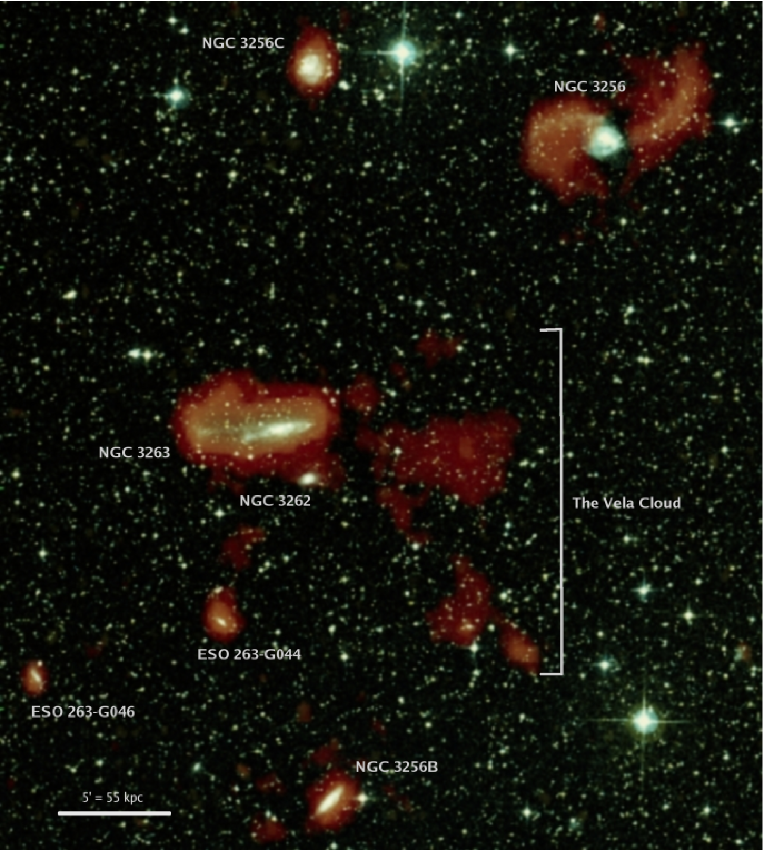
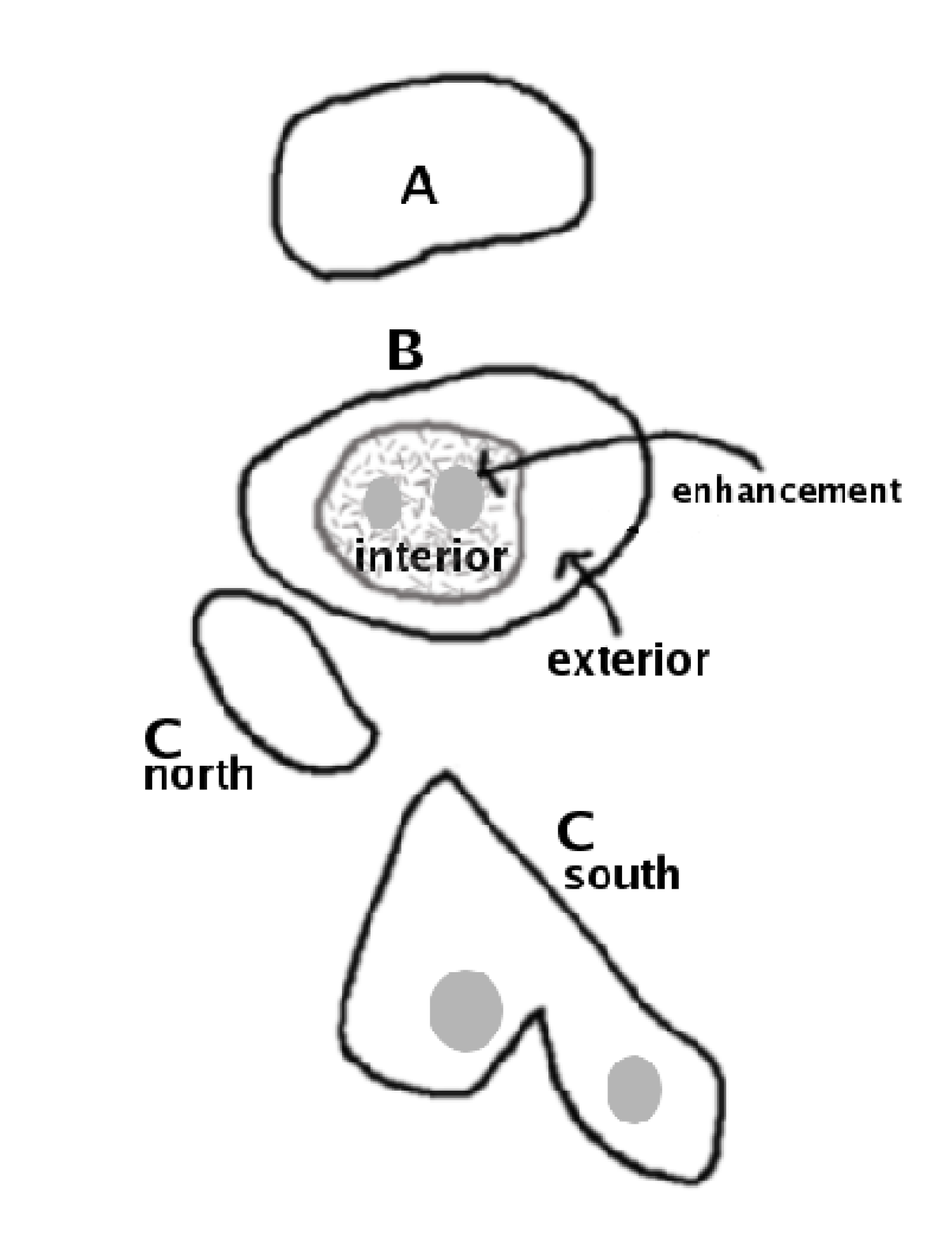
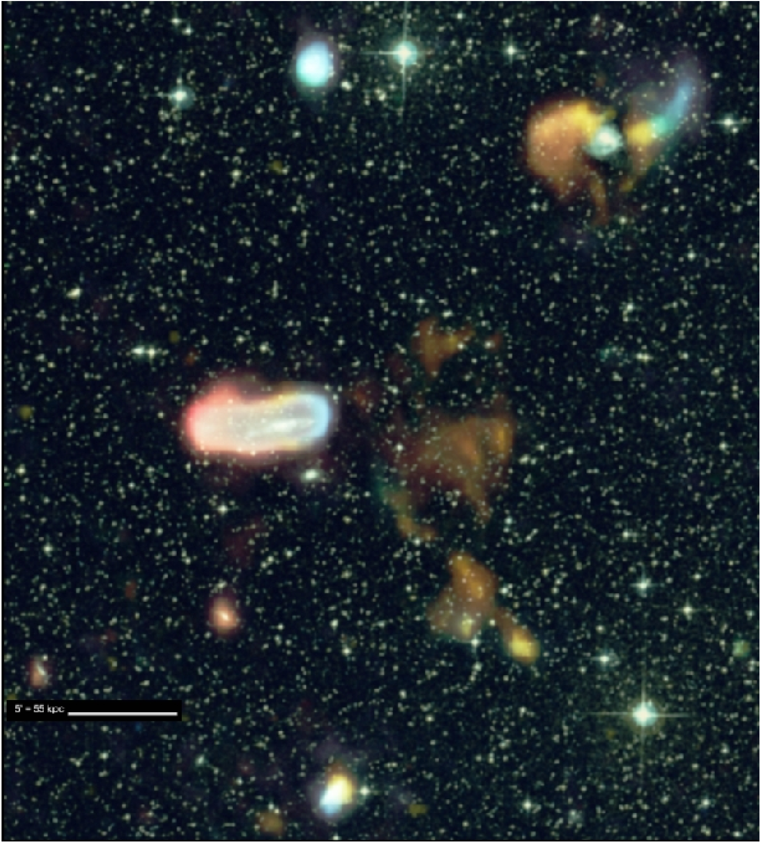
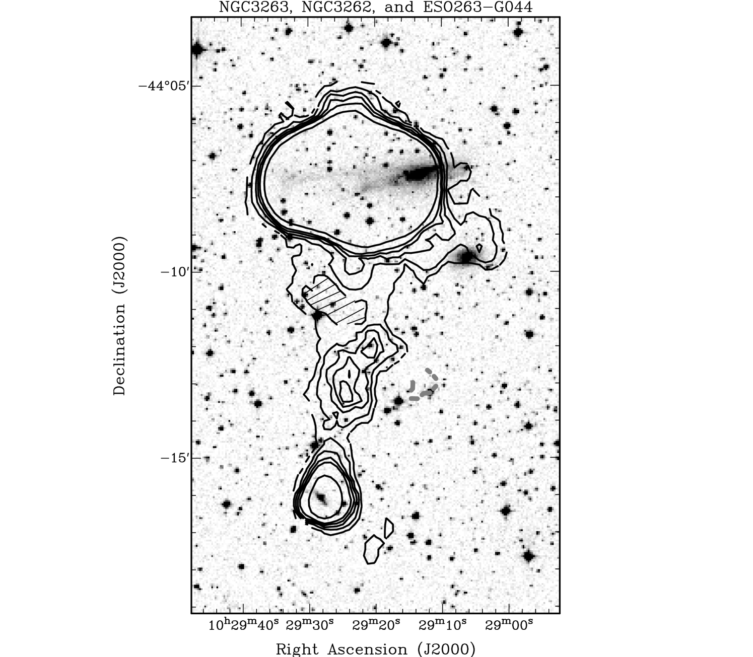
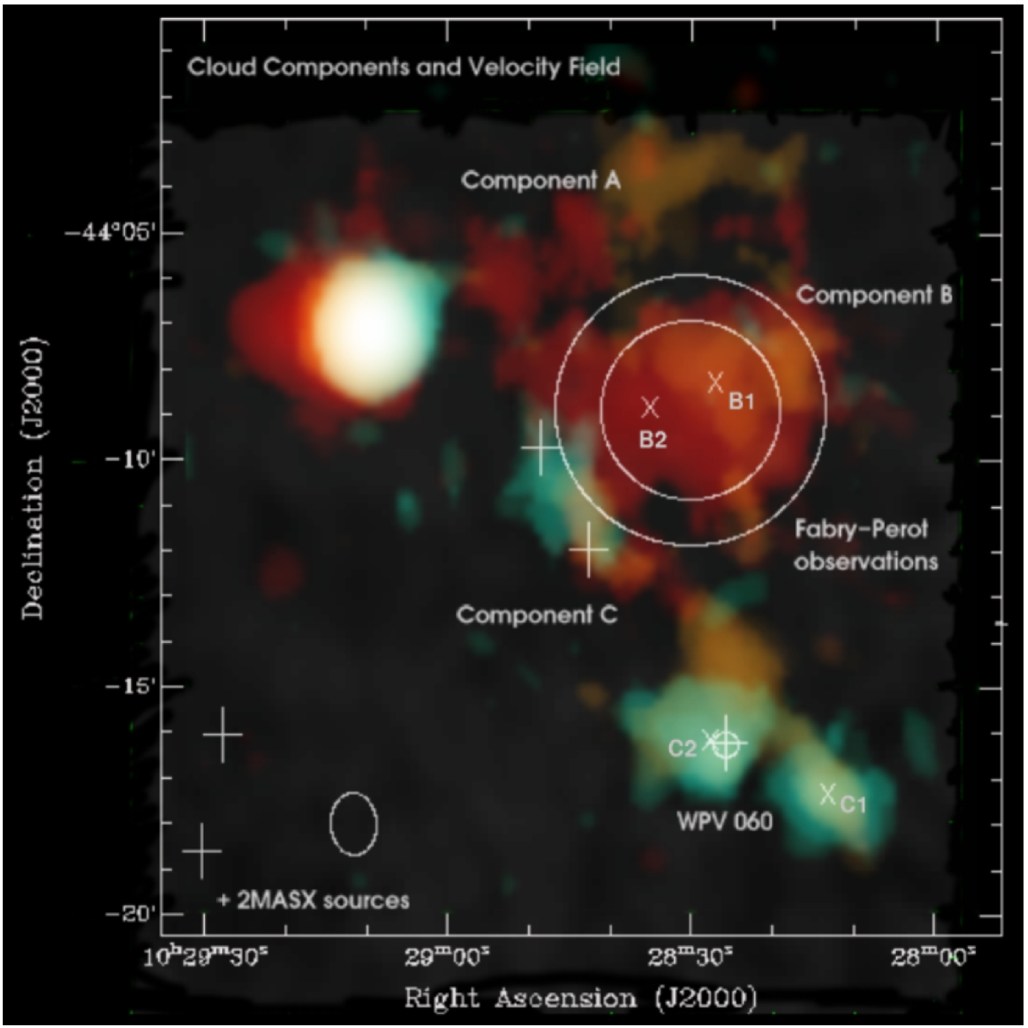
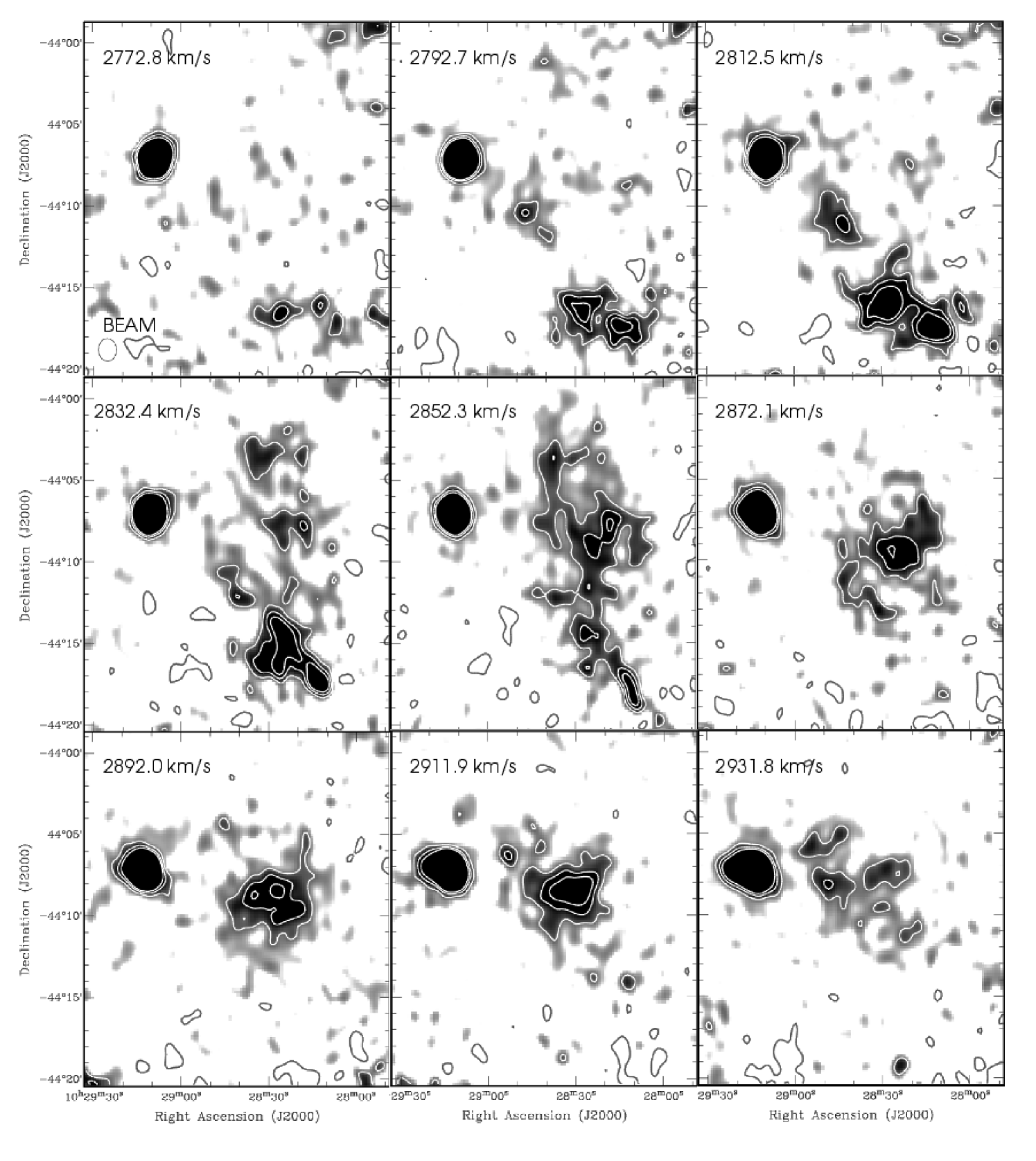
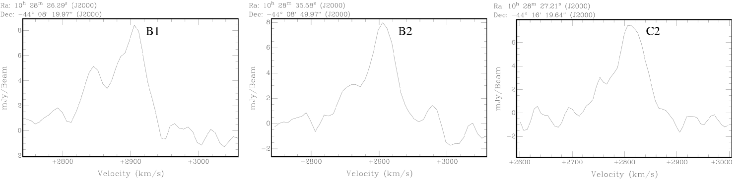
Editor: Please rotate this figure to landscape mode so that the lines show well. Also ensure that it is on a separate page.
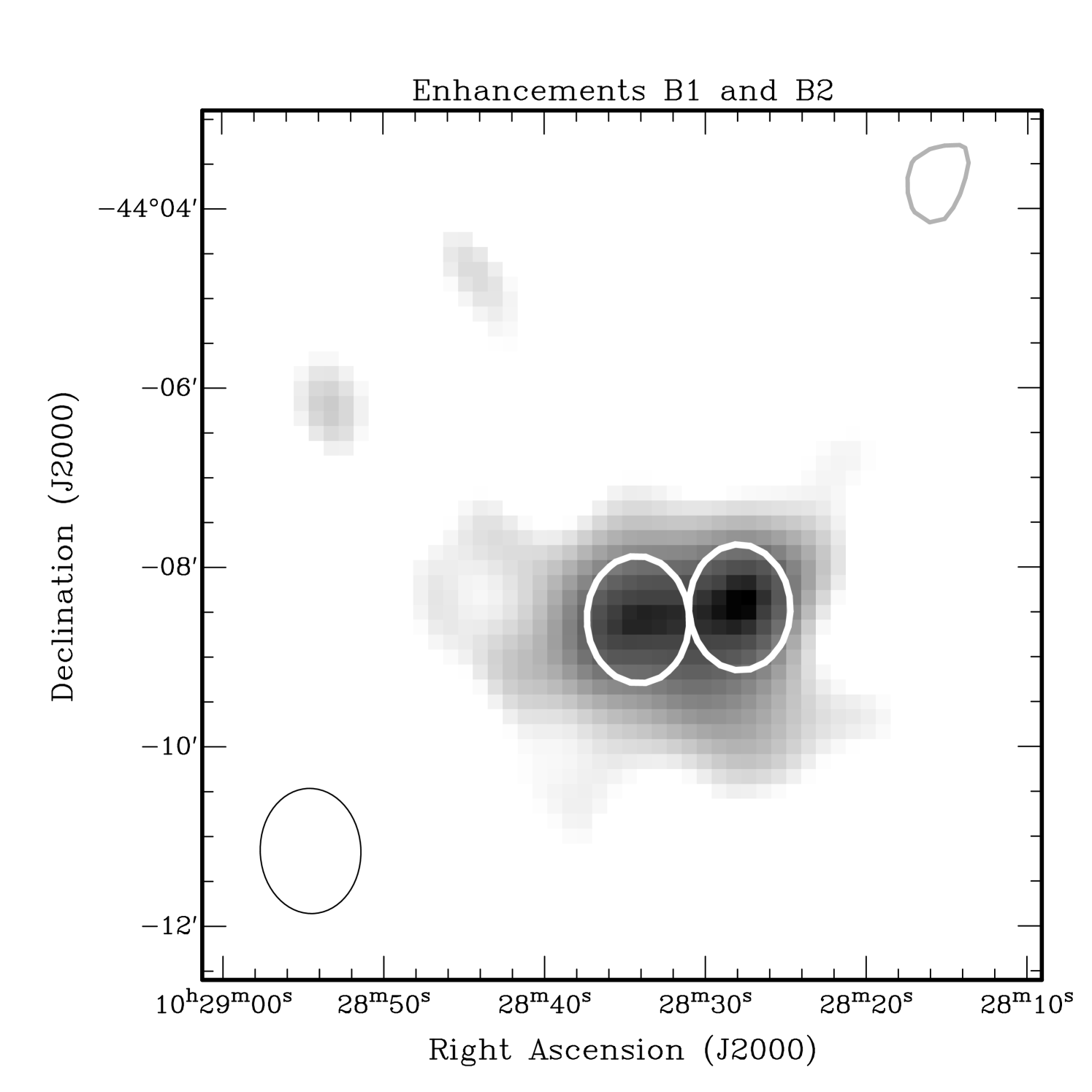
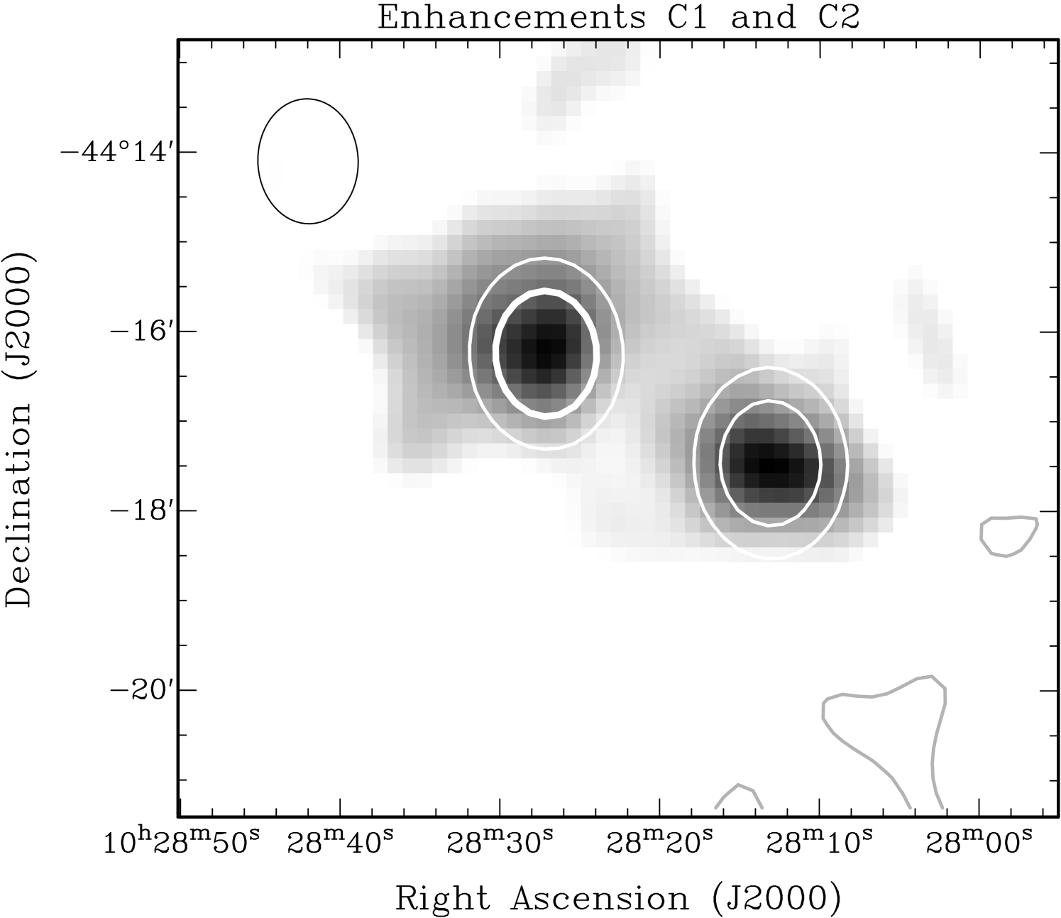
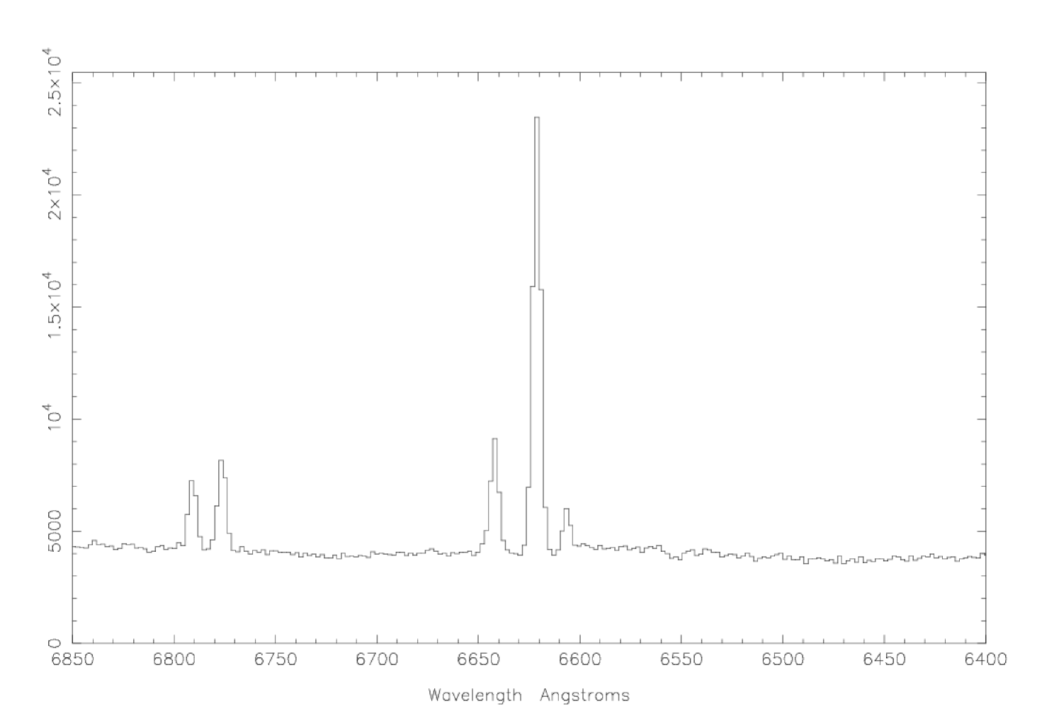
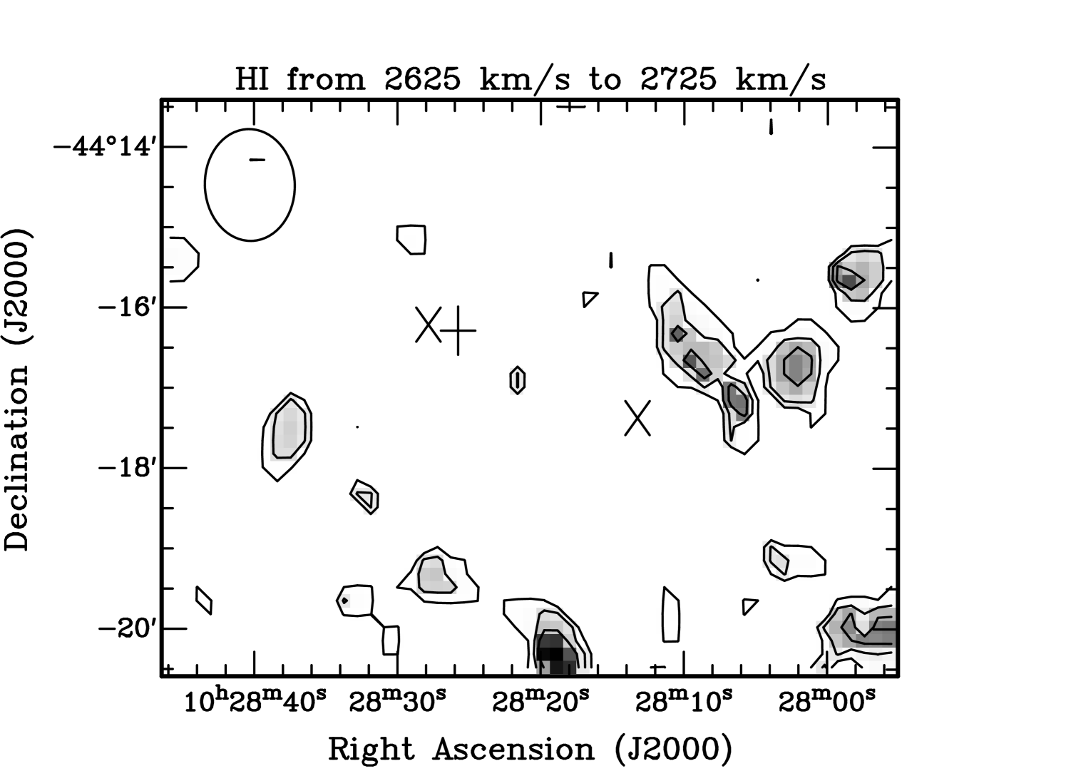
Editor: Please rotate this figure to landscape mode so that the lines show well.
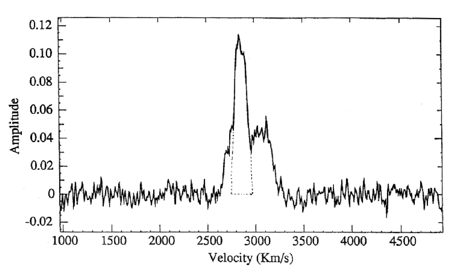
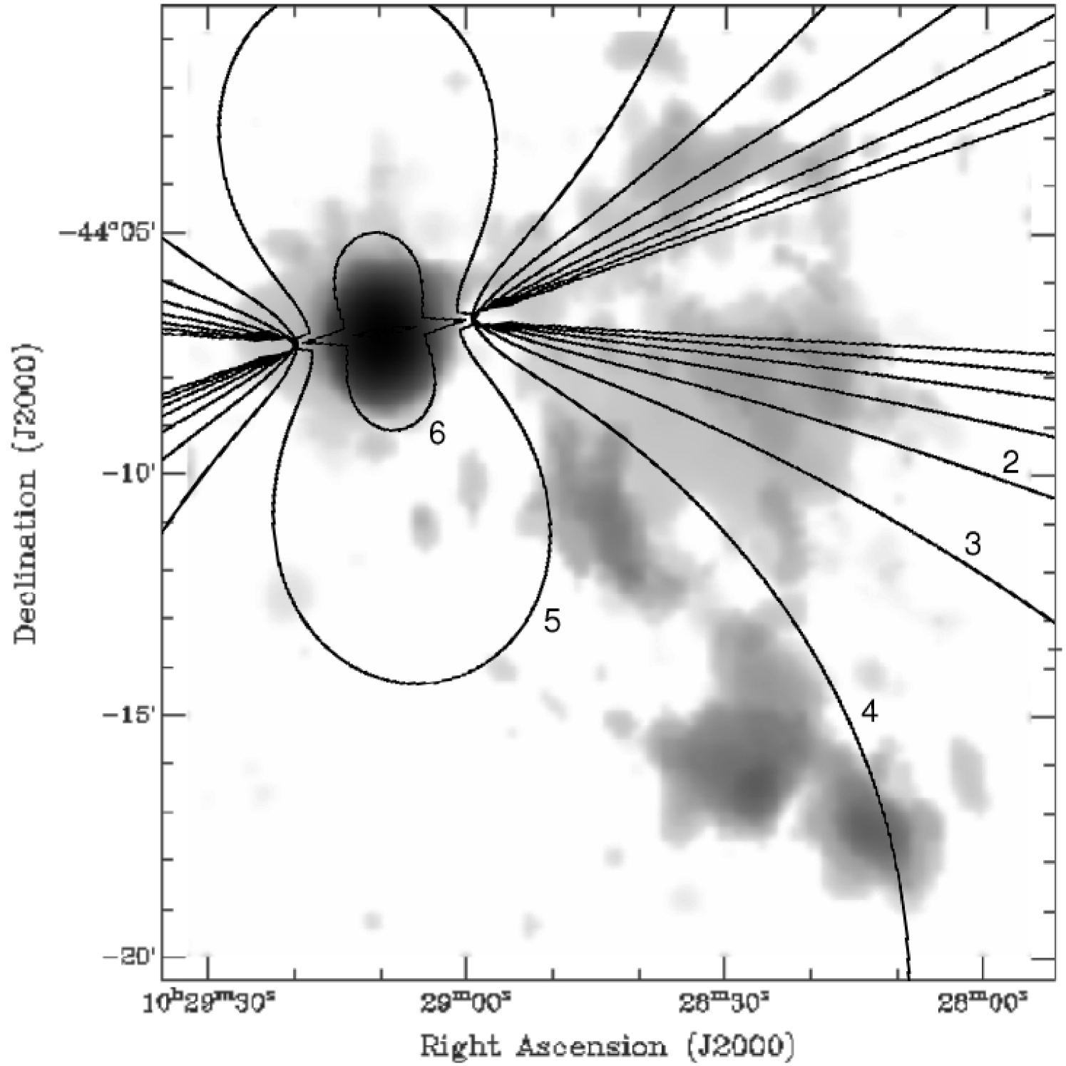
| Parameter | HI Cube |
|---|---|
| Synthesized Beam (arcsec) | 84 x 67 |
| Beam Position Angle | 2.5∘ |
| Channel Width (km ) | 6.6 |
| Weighting | natural |
| Measured aaThe was determined before correction for the primary beam. (mJy ) | 1.3 |
| Total Velocity Range (km ) | 2330 to 3416 |
| Target | Exposure Time (sec) | Airmass | Description |
|---|---|---|---|
| The Vela Cloud | 1200 | 1.3 | target field |
| The Vela Cloud | 1200 | 1.1 | target field |
| The Vela Cloud | 1200 | 1.1 | target field |
| The Vela Cloud | 1200 | 1.0 | target field |
| EG 193 | 120 6 | 1.5 | photometric standard |
| Cloud Component | |||||
|---|---|---|---|---|---|
| A | B | C | |||
| Whole | InterioraaThe central region of component B. See § 5.2.1 and Fig. 2. | Exterior | |||
| Heliocentric Systemic | 2842 4 | 2885 6 | 2905 6 | 2813 7 | |
| Velocities () | |||||
| FWHM ()bbThe uncertainty (§ 3.1) is 10 to 15%. With respect to Cloud C see the end of § 4.1.1. | 41 | 97 | 51 | 97 | |
| Velocity Range | 2832-2852 | 2832-2938 | 2872-2932 | 2786-2839 | |
| () | |||||
| Length (arcsec)ccAt a distance of 37.6 Mpc, 1′′ is equivalent to 182 pc. | 220 26 | 368 18 | 175 5 | 760 10 | |
| Width (arcsec) | 140 14 | 300 20 | 130 9 | 260 10 | |
| Flux Density | 0.47 | 4.2 | 0.77 | 4.9 | |
| (Jy )ddThe uncertainties are(§ 3.1) : flux density ; column density ; peak column density . The uncertainty for mass is (§ 4.1.1). | |||||
| Column Density | 1.10 | 6.83 | 7.45 | 6.67 eeFor cloud C the column density value is the average of the north and south components which, separately, are (north) and (south). | |
| (atoms cm-2)ddThe uncertainties are(§ 3.1) : flux density ; column density ; peak column density . The uncertainty for mass is (§ 4.1.1). | |||||
| Peak Column Density | 2.62 | 1.21 | 1.70 | ||
| (atoms cm-2)ddThe uncertainties are(§ 3.1) : flux density ; column density ; peak column density . The uncertainty for mass is (§ 4.1.1). | |||||
| Mass ()ddThe uncertainties are(§ 3.1) : flux density ; column density ; peak column density . The uncertainty for mass is (§ 4.1.1). | 1.6 | 14.0 | 2.5 | 11.5 | 16.3 |
| Pressure/k ()ffThe uncertainty is 43% (§ 5.2.1). Pressure has been divided by the Boltzmann Constant k. | 5 | 100 | 50 | 91 | 39 |
| Enhancement | B1 | B2 | C1z | C1y | C2 |
|---|---|---|---|---|---|
| Position(J2000)aaThe uncertainty in position is 26″(§ 3.2). | |||||
| (hms) | 10 28 27.2 | 10 28 35.3 | 10 28 13.2 | 10 28 13.2 | 10 28 27.8 |
| (°′″) | -44 08 17 | -44 08 50 | -44 17 28 | -44 17 15 | -44 16 13 |
| Central VelocitybbThese heliocentric radial velocities are the central velocities of single Gaussian profiles, except for C1. C1’s two velocity peaks are labeled z and y and blend at the 50% level. Note, B2 is visually most delineated at 2897 . () | 2906 3 | 2908 | 28077 | 28357 | 2815 3 |
| Peak Intensity r.m.s.ccThis is the number of r.m.s. at which the peak intensity occurs above the mean intensity of the surrounding diffuse host component. See § 3.2. | 3 | 2 | 4 | 3 | 3 |
| FWHMddThe uncertainty includes differences between using smoothed and unsmoothed profiles. () | 31 5 | 28 2 | 20 6 | 21 6 | 44 1 |
| Integrated Flux DensityeeThe uncertainty is 0.06 Jy; § 3.2. (Jy) | 0.26 | 0.23 | 0.28 | 0.22 | 0.40 |
| Enhancements | |||
|---|---|---|---|
| Parameter | B1 | B2 | C2 |
| aa The velocity dispersion in an enhancement is derived using the FWHM listed in Table 4. () | 13.2 | 11.9 | 18.7 |
| bbThe uncertainty is . The measurement is described in § 3.2 and the uncertainty in § 4.2. () | 0.9 | 0.8 | 1.3 |
| ccThe uncertainty is ;§ 5.3. () | 1.02 | 0.69 | 5.68 |
| 11 | 9 | 44 |