The view of TK-SVM on the phase hierarchy in the classical kagome Heisenberg antiferromagnet
Abstract
We illustrate how the tensorial kernel support vector machine (TK-SVM) can probe the hidden multipolar orders and emergent local constraint in the classical kagome Heisenberg antiferromagnet. We show that TK-SVM learns the finite-temperature phase diagram in an unsupervised way. Moreover, in virtue of its strong interpretability, it identifies the tensorial quadrupolar and octupolar orders, which define a biaxial spin nematic, and the local constraint that underlies the selection of coplanar states. We then discuss the disorder hierarchy of the phases, which can be inferred from both the analytical order parameters and a SVM bias parameter. For completeness we mention that the machine also picks up the leading correlations in the dipolar channel at very low temperature, which are however weak compared to the quadrupolar and octupolar orders. Our work shows how TK-SVM can facilitate and speed up the analysis of classical frustrated magnets.
-
August 11, 2025
Keywords: machine learning, TK-SVM, multipolar order, classical spin liquid \ioptwocol
1 Introduction
The kagome Heisenberg antiferromagnet (KHAFM) is one of the most characteristic many-body systems where a simple Hamiltonian hosts strikingly rich physics. A kagome lattice is built from corner-shared triangular plaquettes, as illustrated in Figure 1. By placing Heisenberg spins on each lattice site and coupling the nearest-neighboring spins, one defines a kagome Heisenberg model, . When the interaction is antiferromagnetic, , the system is highly geometrically frustrated and fails to find a unique ground state [1]. Such frustration has played a crucial role in the search for spin liquids and other exotic states of matter [2].
In the most general formulation of the problem one takes the interplay between geometric frustration, quantum fluctuations, and thermal fluctuations into account. However, it turns out that the thermodynamics of the classical KHAFM is already quite rewarding. In Ref. [3], Chalker et al. realized that there exists a hidden quadrupolar order characterized by a rank- tensorial order parameter. The emergence of this order is driven by an order-by-disorder phenomenon [4, 5], where coplanar states are entropically selected at low temperatures owing to the presence of soft modes [3]. Shortly afterwards, Reimers and Berlinsky [6] carried out a thorough investigation of excitations of the soft modes and the correlations of degenerate magnetic states. In spite of limited computational resources the authors showed, by classical Monte Carlo simulations, convincing signatures that the quadrupolar order indeed appears to be (quasi-)long ranged. At around the same time, Huse and Rutenberg [7] and Ritchey et al. [8] proposed that the physics in the selected plane might be effectively described by three-state Potts-like degrees of freedom, and the latter paper also discussed the associated topological defects which can support a generalized Berezinskii-Kosterlitz-Thouless (BKT) transition [9, 10, 11]. This is highly non-trivial, because the BKT transition is not realized in a typical two dimensional Heisenberg magnet as the fundamental group is trivial [12, 13]. It, however, becomes possible with the effective Potts-like degrees of freedom, where the fundamental group is which gives rise to gapped topological defects [13], where () denotes the (binary) dihedral group. Although these results firmly evidenced that there is further structure in the selected coplanar states, it was only much later that Zhitomirsky pointed out that the structure is described by another hidden order, a rank- octupolar order [14, 15]. This author also showed that such order coexists with pinch points, which are usually seen in classical spin liquids such as spin ice [16, 17]. While the quadrupolar and octupolar orders are firmly established, they do not exhaust the rich hierarchy of phases in the classical KHAFM; specifically, the possibility of dipolar order is debated in the literature. Already in Ref. [7], the authors argued that fluctuations around the extensively degenerate KHAFM ground states interact in a non-linear way and will lead to unequally weighted Potts states. As a consequence, there may exist a critical point for a long-range antiferromagnetic order in the limit. This scenario was further developed by Henley with a self-consistent effective Hamiltonian approach [18]. A recent Monte Carlo simulation, equipped with an ingenious cluster update, by Chern and Moessner also suggests that the magnetization retains a finite, though remarkably small, value in the thermodynamical limit as [19].
Whereas establishing the magnetic order is very difficult because of the lack of a controlled theory [18] and efficient algorithms to simulate large system sizes from first principles at extremely low temperature [19, 20], a major challenge in understanding the hidden multipolar orders in the classical KHAFM is rooted in the complexity of those high-rank tensorial order parameters. It is therefore interesting to ask whether machine learning (ML), which is designed to analyze complex patterns, can assist in the analysis of such problems. This also concerns ML techniques as practical tools for physics. Although these techniques have proven useful for classifying phases and detecting phase transitions [21, 22, 23, 24, 25, 26, 27], representing quantum wave functions [28, 29, 30, 31, 32, 33], designing algorithms [34, 35, 36, 37], and predicting properties of materials [38, 39, 40, 41] (see Refs. [42, 43, 44] for recent reviews), the number of applications to intricate issues remains limited.
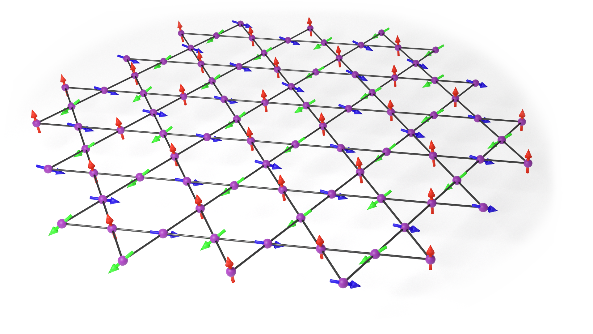
In the present paper, we apply our recently developed tensorial kernel support vector machine (TK-SVM) [45, 46, 47], which is an unsupervised and interpretable approach, to the classical KHAFM. We show that our machine readily picks up the hidden quadrupolar and octupolar orders and gives their tensorial order parameters in analytical form while its only inputs are real-space spin configurations. It identifies the ground-state constraint (GSC) and different temperature scales in the KHAFM. In addition, the machine also recognizes that the magnetic correlation of classical KHAFM at low-temperature is dominated by a structure.
The manuscript is organized as follows. In Section 2, we review the method of TK-SVM. In Section 3, the finite-temperature phase diagram of KHAFM is discussed. Section 4 is devoted to the multipolar order parameters and GSC. Section 5 discusses magnetic correlations. We conclude in Section 6.


2 Tensorial-kernel support vector machine
The tensorial kernel support vector machine (TK-SVM) is a numerical method to detect general symmetry-breaking orders [45, 46] and emergent local constraints [47, 48] in the problem of phase classifications; see also Ref. [49]. It inherits from support vector machines [50, 51], a well-known and successful classifying technique in machine learning, the property that it is interpretable: The decision function, which is the optimal classifier between two sets of data with a distinct property, can be shown to learn the square of order parameters when a quadratic kernel is used [21, 45, 46]. In TK-SVM the order parameter (or local constraint) can be any local tensor of a possibly high rank [45, 46].
Furthermore, the decision function also contains an offset known as the bias. Specifically for phase classification, the bias is sensitive to the presence of phase transitions or crossovers [46, 47]. It can be analyzed prior to and independent of the determination of the order parameters and allows one to perform an unsupervised graph partitioning of the phase diagram.
The main advantages of our approach are that the user does not need to devise suitable order parameters, which are typically very hard to construct for exotic states of matter, and that one gets near certainty about all phases with learned order parameters without supervision, resulting in enormous speedups for the analysis of an (unknown) phase diagram. Below we explain the most important concepts of TK-SVM.
2.1 TK-SVM decision function
The TK-SVM finds the optimal decision function
| (1) |
in classifying two sets of data with a distinct property (e.g. a different order parameter or local constraint) in the sense of determining a maximal margin between the sets.
Here, denotes a real-space configuration of spins, which serves as the training data,
| (2) |
spins are of interest to us, but applications to and Ising spins are straightforward. It plays no role what algorithm has generated the samples .
The power of SVMs lies in the usage of appropriate kernel methods. Samples are mapped by some transformation onto a feature space where only the inner product of the transformed data needs to be known [51]. The conditions on are very mild. Often, a linear separation in feature space is possible, which can correspond to a highly non-linear separation in physical space. In the TK-SVM, maps to degree- monomial configurations,
| (3) |
where ; ; is a collective index; denotes a lattice average up to clusters of spins. This mapping is established by the fact that local orientational orders can be generally represented by finite-rank tensors built from a finite number of vector fields [52, 53, 54]. For example, magnetic orders are defined as rank- tensors, and quadrupolar orders correspond to rank- tensors. Emergent local constraints, such as ground-state constraints for spin liquids, show up as relations between local tensors [47, 48]. The dimension of the -space is . However, as it contains a massive amount of redundant information, the actual complexity in the SVM optimization problem is linearly determined by the number of independent components, given by [45]. While this can still be a big number, a bottleneck is only encountered in extreme situations when dealing with very large clusters at high ranks. In real applications, a TK-SVM can handle, for example, a cluster of several hundreds spins at rank- without a problem, which is only necessary when a quadrupolar order or a spin-liquid constraint has such a vast “unit cell”. In the case of rank , which detects magnetic orders, the size of a feasible cluster can be even greater.
Coefficient matrices, , will be constructed by support vectors,
| (4) |
where is the Lagrangian multiplier related to the -th sample and is solved in the underlying SVM optimization problem. The coefficient matrices can be viewed as encoders of order parameters, from which analytical expressions of the detected orders and constraints are extracted. As we investigated in Ref. [45] by comparing results using to samples, a few hundred samples can already give coefficient matrices of decent quality; more samples reduce statistical errors. The complexity of the underlying SVM optimization problem generally scales as to [55]. However, the computational cost for carrying out the machine learning is in general small compared to that of generating the training data.
The parameter is called the bias. In a binary classification over two sample sets and , its behavior can be summarized as follows [47]
| (5) |
Therefore, the parameter can act as an indicator of phase transitions and crossovers. Its magnitude indicates the absence or presence of a phase transition or crossover,
| (6) |
The sign of further reveals which sample set originates from the (dis-)ordered side, namely, the orientation of the transition or crossover. The last case in Eq. (5) corresponds to situations where and have characteristics that can not straightforwardly be compared; hence, a relative disorderedness may not be well defined.
2.2 Graph partitioning
The use of graph partitioning in TK-SVM maximally exploits the reduced criterion Eq. (6) for . Consider a spin model involving a set of physical parameters such as interactions and temperature, whose phase diagram we seek to learn. We collect spin configurations from distinct parameter points in the physical parameter space. The distribution of the points can be uniform or not in case one wants to have a higher density of points in the regions of special interests. We then perform SVM multi-classification over the collected data. For sets of samples, one multi-classification produces decision functions; each is responsible for a binary classification between two sample sets [56].
The graph is constructed by viewing those parameter points as vertices and assigning an edge to each pair of them, while the edge weights are determined by the value of in the corresponding decision function, leading to a graph of vertices and edges.
The graph may be partitioned by different means. A simple yet efficient approach is Fiedler’s theory of spectral clustering [57, 58]. According to Fiedler’s theory, the graph can be described by a Laplacian matrix . The off-diagonal elements of record the edge weights, and the diagonal elements represent the total weights of every vertex. The second smallest eigenvalue, , of measures the algebraic connectivity of the graph. The eigenvector, , associated with is known as the Fiedler vector and reflects the clustering of the graph. As we shall discuss in Section 3, the Fiedler vector plays the role of a phase diagram.
3 The phase diagram learned by TK-SVM
In order to learn the phase diagram of the classical KHAFM in an unsupervised way, we start the analysis with the graph partitioning. For this purpose, we collect spin configurations ranging from high to extremely low temperatures: we choose logarithmically equidistant temperatures between and , and store independent configurations at each temperature. The samples are obtained by classical Monte Carlo simulations utilizing parallel tempering and heat-bath updates for a lattice consisting of spins ( kagome unit cells) [49].
Next, we apply TK-SVM between any two temperature points and repeat this for different ranks and clusters, which both need to be sufficiently large in order to accommodate the correct orders. In practice, we typically examine clusters comprising a number of lattice unit cells and scrutinize the ranks that are compatible with a crystallographic system (). For the kagome Heisenberg model, it turns out that the optimal choice for learning the quadrupolar and octupolar order is the kagome unit cell (i.e., a three-spin triangle) with ranks and . The results will be compared with those using a single-spin cluster. In Section 5, we will also discuss the rank results of magnetic correlations.
Here are hence four different TK-SVM classification setups (the two types of clusters (a single unit cell and a single spin) combined with the two ranks ( and ). Each leads to a graph of vertices and edges, visualized by Figure 2. The edge weights are defined by a Lorentzian function
| (7) |
where is the bias parameter of the binary classification, and determines a characteristic value for “” in the reduced criterion Eq. (6). The choice of is nevertheless not crucial because vertices in the same phase typically have stronger connections than those from different phases. The robustness of the graph partitioning follows from the fact that can be varied over several orders of magnitude without significant changes to the topology of the phase diagram [47].
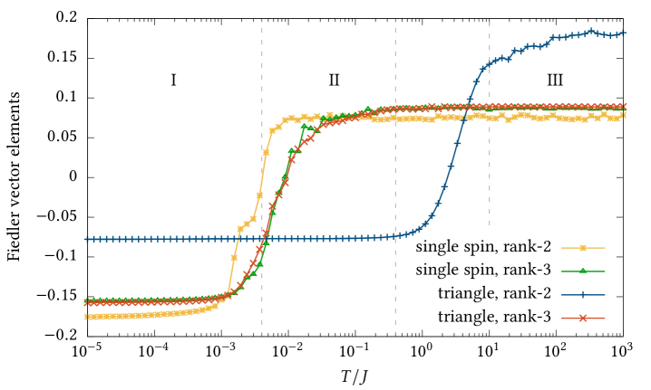
Partitioning these graphs leads to four different Fiedler vectors, depicted in Figure 3. Clearly, the temperature axis is divided into three regions: A rank- quantity constructed from the triangle cluster (see also panel (c) in Figure 2) discriminates around a temperature a high-temperature region (region III) from the rest. Both the single-spin and the triangle cluster (cf. panels (b) and (d) in Figure 2) define a rank- quantity which distinguishes the very low temperatures (region I, ) from the intermediate temperature region II. The result of the single-spin cluster at rank- (cf. panel (a) in Figure 2) is in line with the results the rank- ones. The discrimination of these regions reproduces in fact the finite-temperature phase diagram of the kagome Heisenberg model [15, 3] – even before we visit the nature of those phases.
4 Analytical order parameters
Having learned the topology of the KHAFM phase diagram, we now interpret the nature of each phase by their order parameters and possible local constraints. This will be done by extracting the analytical order parameters from the matrices. In order to reduce the statistical errors on , we pool the data according to the phase diagram of Figure 3. In addition, we introduce fictitious configurations generated at which represent completely disordered states. This sets up a reduced multi-classification problem among four classes: regime I ( samples), regime II ( samples), regime III ( samples), and regime . Consequently, we obtain six for each rank and cluster, with [49].
Not surprisingly, the high-temperature regime III is not distinct from the regime; the associated coefficient matrices are noise-like. Hence, only the two low-temperature regimes need further interpretation.
| on-site | -0.487 | 1.460 | 0.731 | 0.732 | 0.733 | 0.727 | 0.735 | |
| I II | cross | 0.081 | -0.730 | -0.366 | -0.366 | -0.367 | -0.363 | -0.367 |
| bond | 0.038 | 0.365 | 0.183 | 0.183 | 0.183 | 0.182 | 0.184 | |
| on-site | 0.059 | -0.176 | -0.088 | -0.088 | -0.088 | -0.088 | -0.088 | |
| I | cross | 0.910 | 0.089 | 0.044 | 0.044 | 0.044 | 0.044 | 0.044 |
| bond | -0.462 | -0.044 | -0.022 | -0.022 | -0.022 | -0.022 | -0.022 | |
| on-site | 0.000 | 0.000 | 0.000 | 0.000 | 0.000 | 0.000 | 0.000 | |
| II | cross | -0.998 | -0.001 | 0.000 | 0.000 | 0.000 | 0.000 | 0.000 |
| bond | 0.445 | -0.001 | 0.000 | 0.000 | 0.000 | 0.000 | 0.000 |
| I II | c s | -0.166 | -0.500 | -0.500 | -0.500 | -0.500 | -0.500 | -0.500 |
|---|---|---|---|---|---|---|---|---|
| b c | 0.471 | -0.500 | -0.500 | -0.500 | -0.500 | -0.500 | -0.500 | |
| I | c s | -0.504 | -0.499 | -0.502 | -0.502 | -0.502 | -0.502 | |
| b c | -0.508 | -0.492 | -0.495 | -0.493 | -0.493 | -0.493 | -0.493 | |
| II | b c | -0.446 |
4.1 Ground-state constraint
We first discuss the emergent local constraint in the two low-temperature phases, which drives the system to coplanar order and is manifest using the triangular cluster at rank-. The term “emergent” in the current case is intended to distinguish from the trivial constraint of spin normalization . Examples of learning more non-trivial constraints, including previously unknown ones, can be found in Ref. [48] in cases of Kitaev and spin liquids.
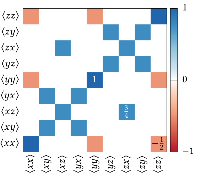
The coefficient matrix is visualized in Figure 4. It is composed of blocks enumerated by the spin indices , with . One easily distinguishes three types of blocks: “on-site” (), “bond” (), and the mixed case “cross”. These blocks can be expressed as
| (8) |
where denotes the ratio between the weight of the on-site and bond quadratic correlations in a coefficient matrix (cf. Table 1 and Table 2), and .
Substituting into the decision function Eq. (1), one obtains
| (9) |
where is a normalized constraint order parameter whose meaning will become transparent in the forthcoming discussion,
| (10) |
As seen in Figure 4 and Table 1, the only non-vanishing quadratic correlation in is
| (11) |
is then determined by for regime II.
The value of in fact appears to be temperature-dependent and converges to in regime I. This can be understood from the constraint order parameter, Eq. (10). As the squared sum in comprises three on-site () and six bond () correlations, and that their ratio is , the fulfillment of is equivalent to the relation
| (12) |
Since is semi-positive definite, this in turn means a local constraint at each triangular plaquette,
| (13) |
Namely, , or equivalently , expresses the ground-state constraint of the KHAFM (the spins of every triangle lie in a plane), while the deviation of in the higher-temperature regime II reflects thermal fluctuations of the constraint.
4.2 Hidden nematic order
We proceed by examining the order parameter of regime I. Given the Fiedler vectors in Figure 3, it is evident that the matrices learned with the single-spin cluster are able to distinguish regime I from the high-temperature phases. We now look at the corresponding coefficient matrices, and will afterwards revisit this issue with the three-spin triangular cluster.
The patterns of using the single-spin cluster are shown in Figure 5, where it is a matrix for rank- and matrix for rank-.
The rank- pattern, shown in Figure 5a, has the following analytic expression,
| (14) |
Substituting this into the decision function Eq. (1), we obtain
| (15) |
where
| (16) |
is the famous uniaxial nematic tensor [59]. This shows that a rank- using a single-spin cluster probes the hidden quadrupolar order in the KHAFM [3, 15].
The rank- pattern Figure 5b is interpreted in the same way. It can be expressed as
| (17) |
leading to a rank- tensor
| (18) |
which is precisely the octupolar order parameter [60].
We are left with the examination of the three-spin cluster. Although it is not quite visible from the Fiedler vector in Figure 3, TK-SVM with a triangular cluster at rank- does in fact discriminate between regime I and II, but the distinction is blurred by the constraint, Eq. (10), which appears as the primary order parameter: The triangular rank- curve in Figure 3 varies in the low-temperature regions, but the gradient is much more modest than the profound change seen when the constraint emerges.
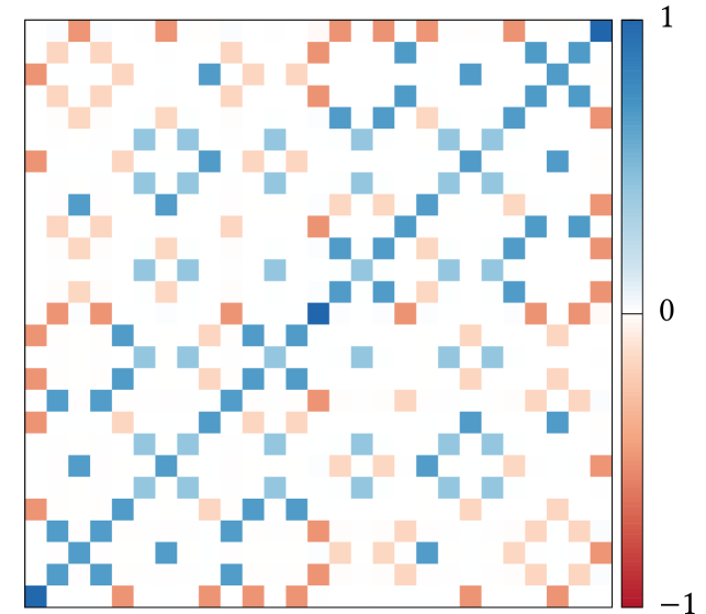
Figure 6 shows the obtained from a three-spin cluster at rank-, which displays a richer structure than the shown in Figure 4. Following a similar analysis, it gives rise to another quadrupolar tensor,
| (19) |
The first term is equivalent to the single-spin nematic tensor Eq. (16), while the second term expresses the constraint, Eq. (13). In other words, the triangular cluster at rank- simultaneously detects the hidden quadrupolar order and the ground-state constraint.
In Figure 7, we show the block structure of the rank- using the triangular cluster. The full matrix has a dimensionality of , which is composed of blocks. Each block exhibits the same pattern as that in Figure 5b for the single-spin cluster, but is further multiplied with a weight. Its analytic expression displays a new octupolar tensor,
| (20) |
The first term of reproduces the single-spin order parameter Eq. (18). The second term represents the ground-state constraint Eq. (13) and will become a constant tensor, , when saturates to , which is the case in regime I. The second term is a rank- tensor defined by the three spins in a triangular plaquette. It serves as an alternative characterization of the octupolar order and is equivalent to the single-spin form. This also explains the agreement of the two rank- Fiedler vectors in Figure 3.
| Cluster | single spin | triangle | ||
|---|---|---|---|---|
| Rank | 2 | 3 | 2 | 3 |
| I II | -1.0131 | -1.0131 | -3.286 | -1.0145 |
| I III | -1.0121 | -1.0041 | -1.0035 | -1.0026 |
| I | -1.0129 | -1.0044 | -0.9928 | -1.0028 |
| II III | 10.63 | -0.9592 | -1.0260 | -1.0691 |
| II | 4.218 | -1.0598 | -1.0103 | -1.0805 |
| III | 2.158 | -1285 | -20.54 | -1.9802 |
4.3 Phase Hierarchy
Let us put the learned order parameters and constraints together and infer a single coherent physical picture. Regime III is a trivial paramagnet (PM) which is equivalent to the infinite temperature state. Regime II is an instance of a cooperative paramagnet (CPM), which may also be referred to as a classical spin liquid and is characterized by an emergent local constraint. Regime I meets the standard of a biaxial spin nematic (BSN) where the uniaxial quadrupolar and the biaxial octupolar order together define the symmetry [53].
Accordingly, the temperature scales in the phase diagram Figure 3 can be understood from a hierarchy of disorderedness,
| (21) |
In the high-temperature PM phase, spins can freely fluctuate. In the intermediate CPM phase, although the system still preserves the symmetry of the KHAFM Hamiltonian, fluctuations of spins become correlated. Then the BSN order emerges from a constrained subset of the phase space.
This phase hierarchy is also reflected by the bias parameters in the four different multi-classification setups, which are shown in Table 3. Following the bias criterion of Eq. (5), regime I (BSN) has the least disorder since in all instances. The learned with the triangular cluster at rank- acquired a value noticeably smaller than , since the constraint Eq. 13 is satisfied in both phases (). However, its sign remains revealing that regime II is more disordered. Regime III (PM) is the most disordered as in all cases, with one exception as the single-spin cluster cannot represent the three-spin constraint Eq. (13).
5 Magnetic correlations
We now examine the magnetic correlations in the low-temperature regime, , of the classical KHAFM, learned by rank- TK-SVM.
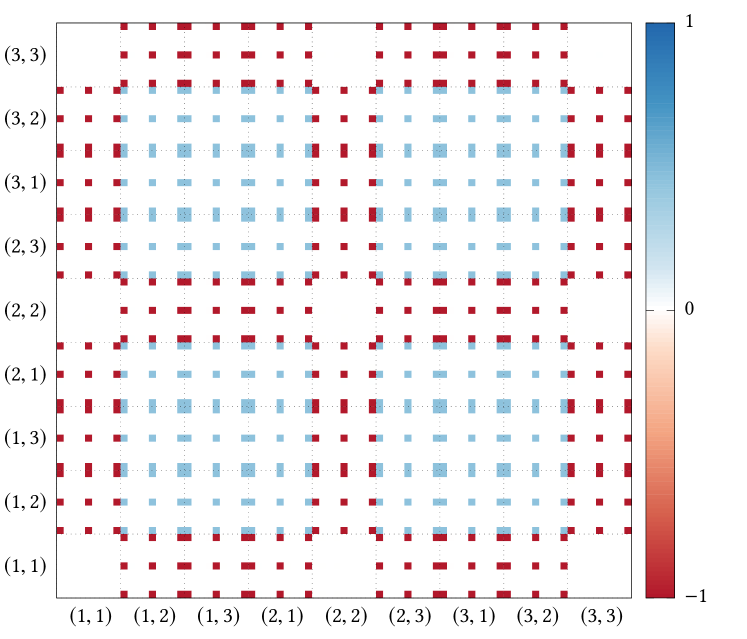
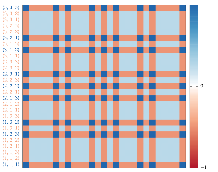
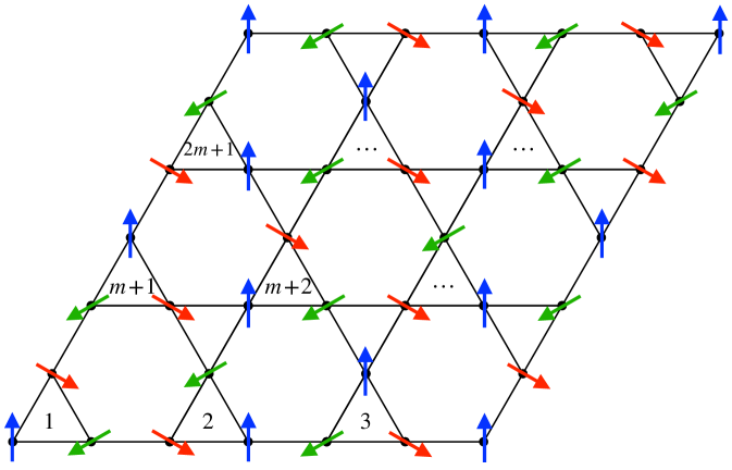
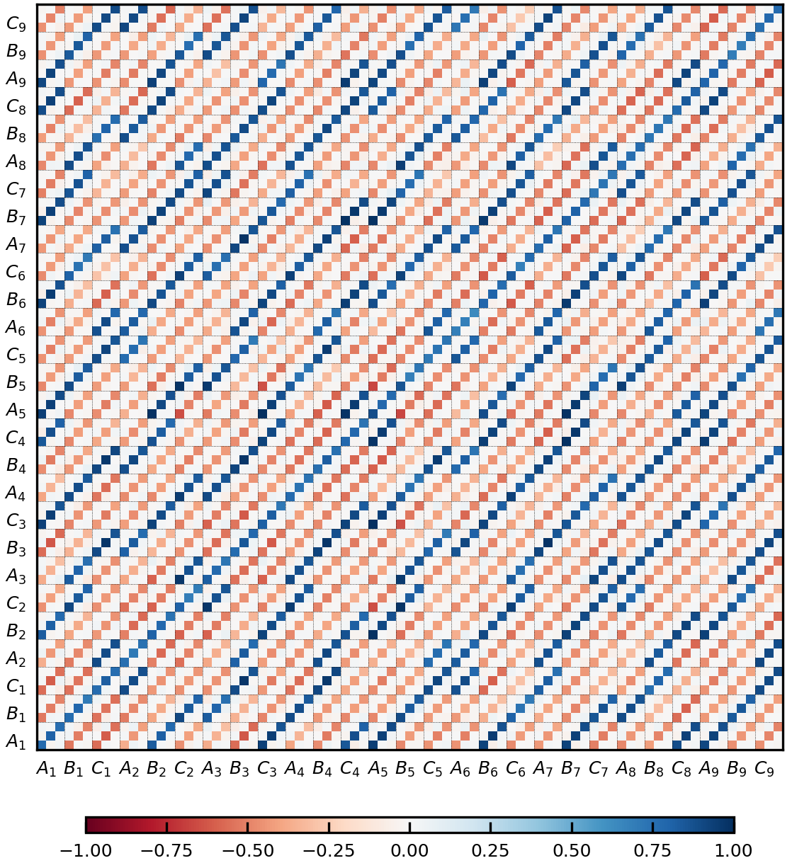
We first consider a cluster containing kagome unit cells, i.e. spins (see Figure 8), for a system defined on a lattice of linear size . The resulting matrix is shown in Figure 9. It has dimension and can be divided into small blocks. The structure of those blocks evinces in which way the correlation between two spins is defined. Because the small blocks have only entries on the diagonal, the correlation is simply captured by the usual inner product . (In general, the contraction can be more complicated even for magnetic orders). The change of color between the blocks indicates an antiferromagnetic arrangement of the spins: The blue blocks correspond to positive correlations, and their locations precisely reflect a structure.
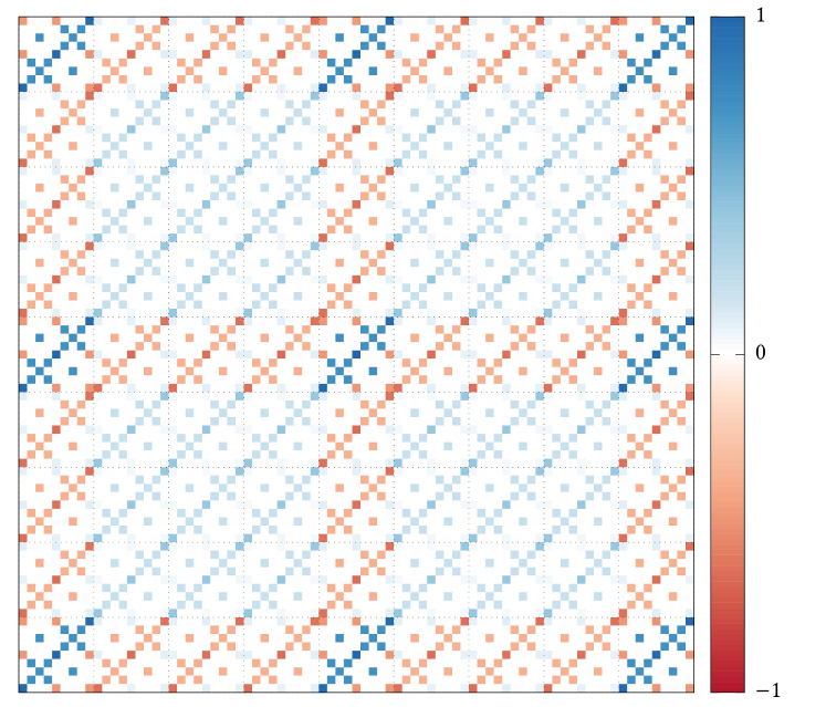
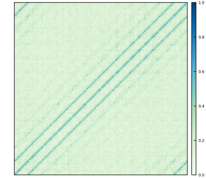
Next, in Figure 10, we show the result using a cluster of kagome unit cells ( spins). Owing to the large dimensionality of the matrix, , only the block structure is plotted, where each of its pixels corresponds to a block in Figure 9. In the presence of long-range order for an order parameter that can be defined on a small cluster, learnt for a large cluster should display the same structure as for that small cluster. However, the pattern of Figure 10 does not repeat that of Figure 9: It fades rather fast, indicating that the linear correlation between two spins is not robustly established at longer distances. (Note that does not directly measure the strength of spin-spin correlations. Instead, it probes the form of the correlations and order parameters. See Eqs. 14 and 4.2 for a concrete example.)
Therefore, consistent with observations in the literature [7, 6, 15, 19, 20], our machine detects that the antiferromagnetic structure is the dominant type of correlation in the dipolar channel of the classical KHAFM at low temperature. However, to establish the critical point, a systematic analysis of temperature and finite-size effect is needed [19], which is beyond the scope of the present paper and current algorithms.
6 Conclusion
In summary, we have shown how TK-SVM can infer the phase diagram of the classical Heisenberg model defined on the kagome lattice in an unsupervised way. It has successfully learned that the spins are constrained to coplanar states owing to an emergent GSC and identified the hidden octupolar and quadrupolar tensor order parameters, which define a biaxial-nematic state. Moreover, the machine also recognized the dominant correlations in the low temperature regime.
As a data-driven approach, it does not require any prior knowledge or particular insight in the system. Instead, by revealing the phase diagram and analytical order parameters in an unsupervised setting, the underlying physics becomes immediately evident. We expect TK-SVM to become an indispensable tool in analyzing many-body spin systems, as it provides an enormous speedup when the order parameters and phase diagrams are complicated.
Open source
The TK-SVM library has been made openly available with documentation and examples [65].
Reference
References
- [1] Lacroix C, Mendels P and Mila F (eds) 2011 Introduction to Frustrated Magnetism (Springer Berlin Heidelberg) URL https://doi.org/10.1007/978-3-642-10589-0
- [2] Balents L 2010 Nature 464 199–208
- [3] Chalker J T, Holdsworth P C W and Shender E F 1992 Phys. Rev. Lett. 68(6) 855–858 URL https://link.aps.org/doi/10.1103/PhysRevLett.68.855
- [4] Villain J 1979 Z. Phys. B 33 31–42 ISSN 1431-584X
- [5] Villain J, Bidaux R, Carton J P and Conte R 1980 J. Phys. France 41 1263–1272
- [6] Reimers J N and Berlinsky A J 1993 Phys. Rev. B 48(13) 9539–9554 URL https://link.aps.org/doi/10.1103/PhysRevB.48.9539
- [7] Huse D A and Rutenberg A D 1992 Phys. Rev. B 45(13) 7536–7539 URL https://link.aps.org/doi/10.1103/PhysRevB.45.7536
- [8] Ritchey I, Chandra P and Coleman P 1993 Phys. Rev. B 47(22) 15342–15345 URL https://link.aps.org/doi/10.1103/PhysRevB.47.15342
- [9] Berezinskiǐ V L 1971 Soviet Journal of Experimental and Theoretical Physics 32 493
- [10] Berezinskiǐ V L 1972 Soviet Journal of Experimental and Theoretical Physics 34 610
- [11] Kosterlitz J M and Thouless D J 1973 Journal of Physics C: Solid State Physics 6 1181–1203 URL https://doi.org/10.1088%2F0022-3719%2F6%2F7%2F010
- [12] Mermin N D 1979 Rev. Mod. Phys. 51(3) 591–648 URL http://link.aps.org/doi/10.1103/RevModPhys.51.591
- [13] Michel L 1980 Rev. Mod. Phys. 52(3) 617–651 URL https://link.aps.org/doi/10.1103/RevModPhys.52.617
- [14] Zhitomirsky M E 2002 Phys. Rev. Lett. 88(5) 057204 URL https://link.aps.org/doi/10.1103/PhysRevLett.88.057204
- [15] Zhitomirsky M E 2008 Phys. Rev. B 78(9) 094423 URL https://link.aps.org/doi/10.1103/PhysRevB.78.094423
- [16] Henley C L 2010 Annu. Rev. Condens. Matter Phys. 1 179–210
- [17] Castelnovo C, Moessner R and Sondhi S L 2012 Annu. Rev. Condens. Matter Phys. 3 35–55
- [18] Henley C L 2009 Phys. Rev. B 80(18) 180401 URL https://link.aps.org/doi/10.1103/PhysRevB.80.180401
- [19] Chern G W and Moessner R 2013 Phys. Rev. Lett. 110(7) 077201 URL https://link.aps.org/doi/10.1103/PhysRevLett.110.077201
- [20] Schnabel S and Landau D P 2012 Phys. Rev. B 86(1) 014413 URL https://link.aps.org/doi/10.1103/PhysRevB.86.014413
- [21] Ponte P and Melko R G 2017 Phys. Rev. B 96(20) 205146 URL https://link.aps.org/doi/10.1103/PhysRevB.96.205146
- [22] Wang L 2016 Phys. Rev. B 94(19) 195105 URL https://link.aps.org/doi/10.1103/PhysRevB.94.195105
- [23] van Nieuwenburg E P L, Liu Y H and Huber S D 2017 Nat. Phys. 13 435–439
- [24] Carrasquilla J and Melko R G 2017 Nat. Phys. 13 431–434
- [25] Liu Y H and van Nieuwenburg E P L 2018 Phys. Rev. Lett. 120(17) 176401 URL https://link.aps.org/doi/10.1103/PhysRevLett.120.176401
- [26] Rodriguez-Nieva J F and Scheurer M S 2019 Nature Physics 15 790–795 URL https://doi.org/10.1038/s41567-019-0512-x
- [27] Zhang Y, Ginsparg P and Kim E A 2020 Phys. Rev. Research 2(2) 023283 URL https://link.aps.org/doi/10.1103/PhysRevResearch.2.023283
- [28] Carleo G and Troyer M 2017 Science 355 602–606 ISSN 0036-8075 (Preprint http://science.sciencemag.org/content/355/6325/602) URL http://science.sciencemag.org/content/355/6325/602
- [29] Huang L and Wang L 2017 Phys. Rev. B 95(3) 035105 URL https://link.aps.org/doi/10.1103/PhysRevB.95.035105
- [30] Cai Z and Liu J 2018 Phys. Rev. B 97(3) 035116 URL https://link.aps.org/doi/10.1103/PhysRevB.97.035116
- [31] Melko R G, Carleo G, Carrasquilla J and Cirac J I 2019 Nature Physics 15 887–892 URL https://doi.org/10.1038/s41567-019-0545-1
- [32] Pfau D, Spencer J S, de G Matthews A G and Foulkes W M C 2019 Ab-initio solution of the many-electron schrödinger equation with deep neural networks (Preprint 1909.02487)
- [33] Hermann J, Schätzle Z and Noé F 2019 Deep neural network solution of the electronic schrödinger equation (Preprint 1909.08423)
- [34] Liao H J, Liu J G, Wang L and Xiang T 2019 Phys. Rev. X 9(3) 031041 URL https://link.aps.org/doi/10.1103/PhysRevX.9.031041
- [35] Carleo G, Choo K, Hofmann D, Smith J E, Westerhout T, Alet F, Davis E J, Efthymiou S, Glasser I, Lin S H, Mauri M, Mazzola G, Mendl C B, van Nieuwenburg E, O’Reilly O, Théveniaut H, Torlai G, Vicentini F and Wietek A 2019 SoftwareX 10 100311 ISSN 2352-7110 URL http://www.sciencedirect.com/science/article/pii/S2352711019300974
- [36] Nagai Y, Shen H, Qi Y, Liu J and Fu L 2017 Phys. Rev. B 96(16) 161102 URL https://link.aps.org/doi/10.1103/PhysRevB.96.161102
- [37] Xu X Y, Qi Y, Liu J, Fu L and Meng Z Y 2017 Phys. Rev. B 96(4) 041119 URL https://link.aps.org/doi/10.1103/PhysRevB.96.041119
- [38] Xie T and Grossman J C 2018 Phys. Rev. Lett. 120(14) 145301 URL https://link.aps.org/doi/10.1103/PhysRevLett.120.145301
- [39] Lee J, Seko A, Shitara K, Nakayama K and Tanaka I 2016 Phys. Rev. B 93(11) 115104 URL https://link.aps.org/doi/10.1103/PhysRevB.93.115104
- [40] Isayev O, Oses C, Toher C, Gossett E, Curtarolo S and Tropsha A 2017 Nature Communications 8 15679 URL https://doi.org/10.1038/ncomms15679
- [41] Zhu Q, Samanta A, Li B, Rudd R E and Frolov T 2018 Nature Communications 9 467 URL https://doi.org/10.1038/s41467-018-02937-2
- [42] Carleo G, Cirac I, Cranmer K, Daudet L, Schuld M, Tishby N, Vogt-Maranto L and Zdeborová L 2019 Rev. Mod. Phys. 91(4) 045002 URL https://link.aps.org/doi/10.1103/RevModPhys.91.045002
- [43] Schmidt J, Marques M R G, Botti S and Marques M A L 2019 npj Computational Materials 5 83 URL https://doi.org/10.1038/s41524-019-0221-0
- [44] Carrasquilla J 2020 Advances in Physics: X 5 1797528 URL https://doi.org/10.1080/23746149.2020.1797528
- [45] Greitemann J, Liu K and Pollet L 2019 Phys. Rev. B 99(6) 060404(R) URL https://link.aps.org/doi/10.1103/PhysRevB.99.060404
- [46] Liu K, Greitemann J and Pollet L 2019 Phys. Rev. B 99(10) 104410 URL https://link.aps.org/doi/10.1103/PhysRevB.99.104410
- [47] Greitemann J, Liu K, Jaubert L D C, Yan H, Shannon N and Pollet L 2019 Phys. Rev. B 100(17) 174408 URL https://link.aps.org/doi/10.1103/PhysRevB.100.174408
- [48] Liu K, Sadoune N, Rao N, Greitemann J and Pollet L 2020 arXiv preprint arXiv:2004.14415
- [49] Greitemann J 2019 Investigation of hidden multipolar spin order in frustrated magnets using interpretable machine learning techniques URL http://nbn-resolving.de/urn:nbn:de:bvb:19-250579
- [50] Cortes C and Vapnik V 1995 Machine Learning 20 273–297 ISSN 1573-0565 URL https://doi.org/10.1007/BF00994018
- [51] Vapnik V N 1998 Statistical learning theory (Wiley) ISBN 9780471030034 URL https://www.wiley-vch.de/en?option=com_eshop&view=product&isbn=9780471030034&title=Statistical%20Learning%20Theory
- [52] Liu K, Nissinen J, Slager R J, Wu K and Zaanen J 2016 Phys. Rev. X 6(4) 041025 URL https://link.aps.org/doi/10.1103/PhysRevX.6.041025
- [53] Nissinen J, Liu K, Slager R J, Wu K and Zaanen J 2016 Phys. Rev. E 94(2) 022701 URL http://link.aps.org/doi/10.1103/PhysRevE.94.022701
- [54] Michel L 2001 Phys. Rep. 341 11–84
- [55] Bottou L and Lin C J 2007 Large scale kernel machines 3 301–320
- [56] Hsu C W and Lin C J 2002 IEEE transactions on Neural Networks 13 415–425
- [57] Fiedler M 1973 Czechoslovak Mathematical Journal 23 298–305 URL http://eudml.org/doc/12723
- [58] Fiedler M 1975 Czechoslovak Mathematical Journal 25 619–633 URL http://eudml.org/doc/12900
- [59] de Gennes P and Prost J 1995 The Physics of Liquid Crystals International Series of Monographs on Physics (Clarendon Press) ISBN 9780198517856
- [60] Fel L G 1995 Phys. Rev. E 52(1) 702–717 URL http://link.aps.org/doi/10.1103/PhysRevE.52.702
- [61] Schölkopf B, Smola A J, Williamson R C and Bartlett P L 2000 Neural Comput. 12 1207–1245
- [62] Chang C C and Lin C J 2001 Neural Comput. 13 2119–2147
- [63] Chang C C and Lin C J 2011 ACM Trans. Intell. Syst. Technol. 2 27:1–27:27 ISSN 2157-6904 URL http://doi.acm.org/10.1145/1961189.1961199
- [64] Gaenko A, Antipov A, Carcassi G, Chen T, Chen X, Dong Q, Gamper L, Gukelberger J, Igarashi R, Iskakov S, Könz M, LeBlanc J, Levy R, Ma P, Paki J, Shinaoka H, Todo S, Troyer M and Gull E 2017 Comput. Phys. Commun. 213 235–251 ISSN 0010-4655 URL http://www.sciencedirect.com/science/article/pii/S0010465516303885
- [65] Greitemann J, Liu K and Pollet L tensorial-kernel SVM library, https://gitlab.physik.uni-muenchen.de/tk-svm/tksvm-op