The virial mode approach to Structure Formation with Warm Dark Matter
Abstract
The small scale structure opens a window to constrain the dynamical properties of Dark Matter. Here we study the clustering of warm dark matter (WDM) in a semi-analytical approach and compared the linear power spectrum of WDM with cold dark matter (CDM) employing a new transfer function in terms of the viral wave number corresponding to a structure with a viral radius , half the size of the free streaming scale radius . The virial mass contained in this structure corresponds to the lightest structure formed for a WDM particle becoming non-relativistic at the scale factor with the corresponding . The viral transfer function is given in terms of the viral mode and two constant parameters and . We compare with the Boltzmann code CLASS for WDM in the mass range 1-10 keV and we obtain the constraint with . In the standard approach the transfer function is given by [2] where encodes the dynamical properties of WDM and must be numerically adjusted by means of a Boltzmann code. In contrast, in our viral approach the physical quantity is simply given in terms of the free streaming scale and can be analytically determined. Our viral proposal has a good agreement with CLASS and improves slightly the results from the standard transfer function. To conclude, we have proposed a new physically motivated transfer function where the properties of WDM are encoded in the viral wave number , is straightforward to determine and improves the prediction of WDM clustering properties.
1 Introduction
The standard CDM model has been a very successful model to describe our Universe and is consistent with cosmological observational evidence such as the cosmic microwave background (CMB) anisotropies [4], galaxy redshift surveys [5], type Ia Supernovae [6] reach to the conclusion that the content of the Universe is composed of 69% dark energy driving the accelerated expansion of the Universe, 31% matter whose clustering feature influence the large scale structure formation, corresponding to 27% Dark Matter (DM) and the remaining 4% is baryonic matter.
The nature of dark matter has received a great deal of attention in the last decade, due in part of the missing satellites in the universe, and the amount of structure at different scales and redshifts puts strong constraints on the nature of dark matter. In recent times the large surveys such as SDSS-IV [7] and in the near future, DESI [8] in the near future will have an important impact in determining the properties of dark energy (DE) and dark matter (DM). Despite the efforts in both particle physics and cosmology, the nature and composition of the DM are still unknown. Candidates for DM can be classified according to its velocity dispersion, , when the DM particle become non-relativistic (given by the scale factor ). For thermal relics one can relate the mass of the WDM particle to . In this case DM is cold for mass larger than (MeV). This kind of DM particles stop being relativistic and start clustering object at early times. DM with a mass around (keV) are known to be warm, WDM, whose main attribute is that its dispersion velocity wipes out some density concentrations of matter and, therefore, induce a cut-off scale into the mass halo function [9]. The amount of energy density today along with the scale factor when the WDM particle becomes non-relativistic are crucial for determining the properties of the large scale structure of the universe. For instance, the dispersion velocity of DM particles wipes out density concentrations of matter and, therefore, induce a cut-off scale in the mass halo function [9]. Most DM candidates have a smooth evolution of the DM velocity, however, phase transitions in the underlying particle physics model for dark matter shows that an abrupt transition to a non-relativistic limit is plausible [10, 11].
The large velocity dispersion of DM at early stages on the evolution of the Universe tends to suppress gravitational clustering at small scales and conciliates with what it is observed. Cosmological N-body simulations of the CDM model predict the number of satellite galaxies in Milky Way-like galaxies is smaller than the expected, the so-called missing satellite problem [12, 13, 14] and high concentrations of DM in the innermost regions of galaxies (cusp-core problem [15, 16]). Baryon physics also pursued the solutions to this problem by integrating star formation and halo evolution in the galaxy, however, the discussion is still in progress [17, 18, 19]. The details of the suppression at small scales depend on the DM particle nature, which takes us to connect the DM models and astrophysical observations. It can be determined by the parametrization of the transfer function in terms of the power spectrum of DM particles and CDM model, where is scale and time-dependent. Is has been conventional to compare the and CDM models at the epoch when the amplitude of the fluctuations of model is half the size of CDM , i.e. . Different ansatzes have been proposed to parametrize the transfer function and the parameters involved must be numerically fitted using numerical Boltzmann codes [2, 3].
Here, we will present a new approach to structure formation where the virial radius places a dominant role in structure formation. This new approach is physically motivated and is consistent with previous works in WDM structure formation and it allows for an understanding of the suppression of small scale structure in terms of the virial mass and radius. We introduce a new analytical transfer function, physically motivated, that reproduces the clustering of large classes non-thermal DM models and preserving the connection with the physics and nature of the DM.
2 Warm Dark Matter
The clustering properties of Dark Matter have a direct impact on the number of halo as a function of mass and redshift and can be contrasted with several observational large scale structure experiment as [7]. The velocity dispersion of DM particles plays a crucial roll in structure formation. While DM particles are still relativistic, primordial density fluctuations are suppressed due to the velocity dispersion of DM particles and inhibit the formation of structure below the free streaming scale [20]. Here, we will present two approaches to extract cosmological clustering properties of warm dark matter (WDM) in terms of Transfer Function defined as the quotient of the linear matter perturbations between WDM and CDM. We refer to the standard approach the work of M. Viel et al. [2, 21] presented in section 2.1 while our virial approach is given in section 3.
Throughout this paper, we adopt Planck 2018 cosmological parameters [4] in a flat Universe with , and as the CDM matter and baryonic with (with ) and the Hubble constant in units of 100 km s-1Mpc-1, the reionization redshift , the tilt of the primordial power spectrum and with the amplitude of primordial fluctuations.
2.1 Transfer Function: Standard Approach
We will now present the standard approach to extract cosmological clustering properties of warm dark matter (WDM) using the Transfer Function defined as the quotient of the linear matter perturbations between WDM and CDM. The velocity dispersion of dark matter particles inhibits the formation of structure and the main parameter to account for this dispersion is the scale factor when these particles become non-relativist given by [20] and recently in [11]. The evolution of the linear energy density fluctuations are conveniently calculated by publicly available Boltzmann codes, e.g. CAMB [22] and CLASS [1], giving a power spectrum of matter-energy density fluctuations . By comparing the power spectrum for different types of WDM particles one can infer the properties of a new WDM model without the need to implement the new model in the Boltzmann codes. The parametrization of the matter power spectrum for different WDM models has been presented in [2, 3], where the properties of WDM models can be studied employing the transfer function , defined as
| (2.1) |
by comparing the power spectrum in the WDM model with CDM. The clustering properties of WDM are conveniently determined by the scale mode, where the power spectrum of the WDM model is suppressed by compared to a CDM model, i.e.
| (2.2) |
and it is a convenient reference point, in Table 1 we show some values for different WDM models. The standard transfer function for thermal WDM particle is given by [3, 2, 20, 23, 24]
| (2.3) |
The clustering properties of the dark matter model is contained in while and are constant parameters to be fitted from numerical simulations. The quantity has been estimated in [3, 2]
| (2.4) |
We can take and as independent parameters or constrain them to be proportional to a single parameter as in [2] where they find
| (2.5) |
with .
2.2 Analysis with mode
Alternatively to , we can define the mode rendering . From Eq.(2.3) we see that the half mode is proportional to
| (2.6) |
with a proportionality constant
| (2.7) |
For the values given in eq.(2.5) we obtain . We define the mode
| (2.8) |
and . We see that for the transfer function takes the constant value
| (2.9) |
with for .
The ratio of the transfer function but . Since is larger than it corresponds to a less linear mode with a smaller transfer function indicating a larger deviation from CDM model. The information using or and is the same and provides an alternative mode to compare WDM models using the transfer function.
3 The Virial Model
We propose to determine the transfer function as a function of the viral mode , defined in terms of the free streaming mode with with half the radius of as structure with a size of the free streaming scale . We refer to he transfer function as the virial approach. The free streaming scale and mass are
| (3.1) |
with and present matter content of the universe. The virial mode, radius and viral mass are given by
| (3.2) |
The mass contained in the virialized structure is conserved and the virial mass is and since is half the size of the density of the virial sphere is . Of course, a halo density profile such as NFW [25, 26] for example, would be more appropriate to determine the energy density inside this structure but this lies beyond the scope of this work. We take the transfer function for the virialized mode as a two-parameter linear transfer function as a function of the viral mode , similar as the Standard Transfer,
| (3.3) |
with and constant parameters. We determine the values of these parameters in the next section (3), where we find that and are correlated leaving with only one free parameter.
3.1 Transfer Function: Virial Approach
Let us now determine compare the transfer function with Boltzmann codes for different WDM models.
| (3.4) |
with and constant parameters. All the physical properties of WDM are imprinted in the virial mode which is directly related to the free-streaming scale given in eq.(4.7) and it is not adjusted by the Boltzmann codes, contrary to the parameter in eq.(2.4) in section 2.1. The dependence of in the transfer function in eq.(3.3) is given by
| (3.5) |
The scale corresponds to a radius which is half the size of the free streaming scale radius . We therefore have virial radius and mode
| (3.6) |
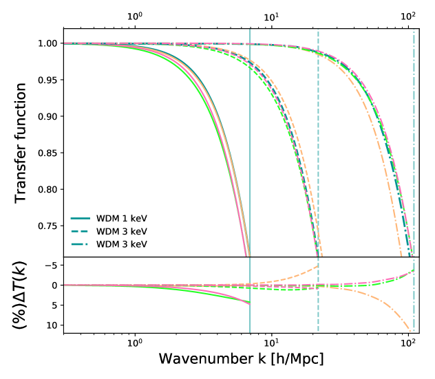
The dependence of the transfer function on the mass of the WDM particle is in the virial mode, , and not in the parameters of the transfer function as in eq.(3.3)). The mode can be easily determined since it is proportional to the free streaming scale (cf. eq.(4.1)) and does not require to be fitted using a numerical Boltzmann code. To determine the values of and we compare our transfer virial function with WDM models from Class code [1], see Fig.2.
We found numerically convenient to define the parameters and as and and we take and as the independent parameters and we obtain for WDM masses in the range (1-10)keV using CLASS, using the result for given in eq.(4.10) to compute and ,
| (3.7) |
| (3.8) |
giving a constraint . We also consider the case with a single free parameter, as in the standard approach, by relating and . Contrary to the ansatz in the standard transfer function approach, here we choose to define and giving a constraint
| (3.9) |
with
| (3.10) |
Notice that the value of in the one parameter case in eq.(3.10) is consistent with the two parameters in eq.(3.8) and allowing us to work with the transfer function in eq.(3.9).
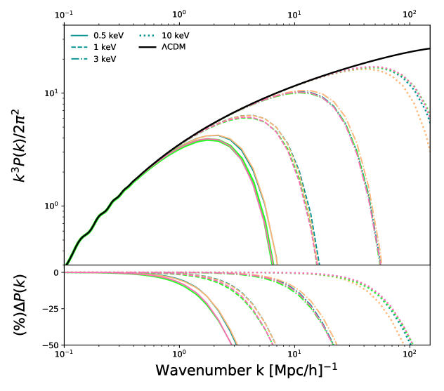
In Table 1 and Fig.2 and Fig.1 we show how good the virial transfer functions is by computing the for different models, for the standard transfer function, , and also the virial approach with 2 free parameters, eq.(3.7) denoted as and with 1 free parameter, eq.(3.9) and denoted as . The numbers is parenthesis are the percentage difference in comparison with the scale directly obtained from the numerical solution from CLASS, . Class code [1], see Fig.2. We show in table 2 the values of and or different WDM masses in the range 1-10keV in our viral approach.
| Mass | ||||||
|---|---|---|---|---|---|---|
| 1 keV | 31.58 | 6.53 (5.60%) | 6.53 (5.60%) | 6.92 (0.11%) | 6.91 | |
| 2 keV | 69.78 | 14.40 (4.40%) | 14.47 (4.88%) | 14.93 (8.25%) | 13.79 | |
| 3 keV | 104.98 | 21.64 (1.03%) | 21.73 (0.58%) | 23.37 (6.88%) | 21.86 | |
| 4 keV | 161.82 | 33.40 (3.60%) | 33.40 (3.60%) | 32.21 (7.03%) | 34.65 | |
| 5 keV | 223.48 | 46.26 (6.05%) | 46.26 (6.05%) | 41.31 (5.29%) | 43.62 | |
| 6 keV | 280.32 | 58.00 (5.61%) | 58.00 (5.61%) | 50.41 (8.20%) | 54.91 | |
| 7 keV | 339.04 | 70.13 (1.44%) | 70.13 (1.44%) | 59.86 (13.41%) | 69.13 | |
| 8 keV | 399.62 | 82.53 (5.17%) | 82.53 (5.17%) | 69.50 (20.15%) | 87.03 | |
| 9 keV | 461.86 | 95.39 (9.60%) | 95.39 (9.60%) | 79.24 (8.95%) | 87.03 | |
| 10 keV | 519.30 | 107.29 (2.08%) | 107.29 (2.08%) | 89.13 (18.65%) | 109.57 |
3.2 Analysis with the Viral mode
For the transfer function takes the value , independently of the value of , and can be used to compare different DM models as (c.f. eq.(2.8)) given in the standard approach. From eq.(3.3) the half mode (i.e. ) is given by
| (3.11) |
with
| (3.12) |
with a constant value given by using eq.(3.10).
| Mass | ||||
|---|---|---|---|---|
| 1 keV | 99.8 | 31.5 | ||
| 2 keV | 43.3 | 72.6 | ||
| 3 keV | 26.4 | 118.8 | ||
| 4 keV | 18.6 | 168.7 | ||
| 5 keV | 14.2 | 221.5 | ||
| 6 keV | 11.3 | 276.9 | ||
| 7 keV | 9.4 | 334.6 | ||
| 8 keV | 8.0 | 394.2 | ||
| 9 keV | 6.9 | 455.6 | ||
| 10 keV | 6.1 | 518.7 |
3.3 Comparing the two approaches
We have presented and alternative approach to the Transfer function. In the standard transfer function approach in section 2.1 the quantity given in eq.(2.4) contains the properties of DM model such as its mass (which can be related to the scale factor when it becomes non-relativistic for thermal WDM particles), however the numerical values have been numerically fitted using a Boltzmann code [2]. In our virial approach, all model dependence is encoded in the free-streaming scale , which is well defined function and is not numerically fitted.
We plot the Matter Power Spectrum and the transfer functions in Fig.1 in the mass range (1 - 10) keV for WDM. Notice that the standard error for all three parameters are small, specially for and . The value of is actually close to previous works that obtained [2], however we find a significantly difference with compared to . The difference in these parameters is because we take a different reference mode instead of as in Viel et al. [2] with similar proportionality constants and .
Our transfer function is physically motivated and is determined in terms of the virial mode which has a clear interpretation in terms of the free streaming scale and in contrast with the fitted parameter (c.f. eq.(2.4)) in the standard approach [3, 2]. Our transfer function has an excellent agreement once we compare with the Boltzmann numerical code, CLASS and it out performs the standard Transfer function in eq.(2.3) for massive particles in the range 1-10keV .
4 Free-streaming scale and Virial radius
The thermal velocities of the dark matter particles have a direct influence on structure formation. While DM particles are still relativistic, primordial density fluctuations are suppressed on scales of order the Hubble horizon at that time. This is called the free-streaming scale and depends on the time when a massive particle becomes non-relativistic . It is defined by
| (4.1) |
The corresponding free-streaming scale mode and a mass contained in sphere of radius are given by
| (4.2) |
and in terms of the viral mode
| (4.3) |
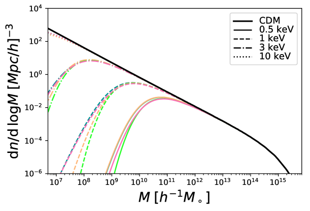
with . For mass-scales the free-streaming of particles erases all peaks in the initial density field therefore the number of structures below this mass scale should be significantly reduced in numbers. We show this behavior in Fig. 4, where we compare CDM and WDM mass functions. However, it is the virialized scale that accounts for the mass contained within the structure to be formed.
4.1 Free Streaming scale
It is conventional to report the free streaming scale assuming a relativistic regime with for and following a non-relativistic regime () with . With these choices of one gets the free streaming scale
| (4.4) | |||||
| (4.5) |
to be compared with of Eq.(4.7) or its limit eq.(4.8). However, we prefer to follow our previous approach [11, 27] and define the time when a particle stops being relativistic, at scale factor , when with the momentum of the particles. The velocity in an expanding universe evolves as
| (4.6) |
which gives a velocity . Eq.(4.6) describes the exact velocity evolution of a decoupled massive particle. The transition between relativistic to non-relativistic is smooth and continuous, see [11] for a generalize transition. This evolution is general and valid for any massive decoupled particles (WDM, CDM or massive neutrinos). Using eq.(4.6) in eq.(4.5) we get [11])
| (4.7) |
which gives free streaming scale without approximation. However, for presentation purposes let assume that and then
| (4.8) |
Here, we use in our calculations eq.(4.7) but for presentation purposes we take the approximations in eq.(4.8). We express and to obtain
| (4.9) |
where has been previously computed in [11],
| (4.10) |
where we consider the DM particle as a fermion with degrees of freedom. With a simple analytic approach for a massive particles characterized by having a non-negligible thermodynamic velocity dispersion [20, 23, 24, 2, 29, 30, 31, 32, 33, 34, 35, 36, 37] we can compute the fluid approximation for the perturbation equations for any massive particles, given the analytic solution for the energy density evolution we were able to reproduce the most appealing feature of WDM, the cut-off in the matter power spectrum [23, 24, 2, 3]. The percentage difference between the numerical value obtained from Boltzmann equations and the analytic one of is on average 3% in a mass range 1-10 keV.
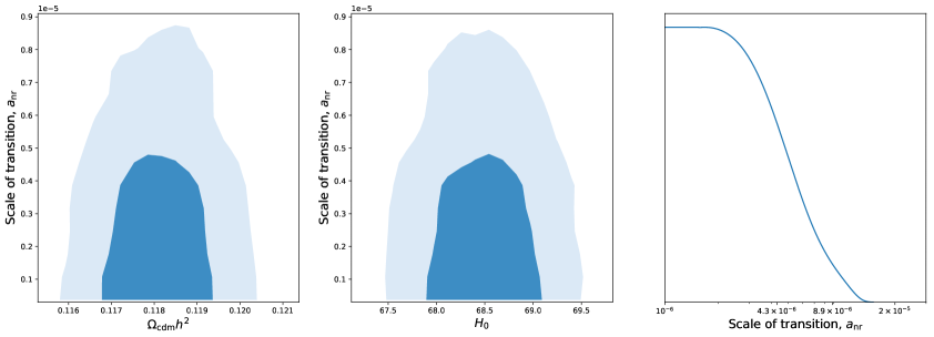
In Table 2 we show different values of and in Fig. 3 we show the lower limits that constrains from the fluid approximation [27] applied to WDM. The free-streaming scale and mass in the limit take the following values
| (4.11) |
with for , and a contained mass of
The virialized structure has a mass , however the energy density in the virialized structure is eight times larger than in , and a radius with
| (4.12) | |||||
| (4.13) |
4.2 Halo Mass Function
The comoving number density of collapsed structure is computed using the Press-Schechter formalism [38]. With the linear matter power spectrum obtained from the transfer function, eq.(2.1), we compute the halo mass function having mass range to as
| (4.14) |
where is the number density of haloes, the halo mass and the peak-height of perturbations is given by , where is the critical overdensity required for a structure to collapse in a dark matter halo in the CDM cosmology. The average matter density is . The corresponding variance of the smoothed density fluctuation in a sphere of radius enclosing a mass is , can be computed from the following integrals
| (4.15) |
Here we will use the sharp-k window function , with being a Heaviside step function (smoothes the large scale mass distribution to a continuous density field), and , where the value of is proved to be best for cases similar as the WDM [39]. Finally, for the mass function, , we adopt [40] that is giving as
| (4.16) |
with , , and determined from the integral constraint .
Using the matter power spectrum using the transfer function with Eq.(2.1), and using the virial approach Eqd.(3.9) and (3.7). We compute the halo mass function, see Fig.4, and compare it with the mass function obtained from CLASS numerical solutions to the matter power spectrum and the same from Viel transfer function, Eq.(2.3).
5 Summary and Conclusion
We studied the clustering properties of WDM particles and we present the viral approach, where the transfer function depends on the viral wave number , and we compare it to the standard approach. The velocity dispersion of WDM at early stages on the evolution of the universe suppress gravitational clustering and may conciliates observations of the number of small scales galaxies. The details of the suppression depend on the properties of the DM particles, however a key ingredient is the time when these particles become non-relativist given by the scale factor .
We have presented here a new approach to structure formation where the virial radius places a dominant role. The viral mode is defined in terms of the free streaming scale and depends thus directly on . This new approach is physically motivated, is consistent with previous works in WDM structure formation, and allows for an understanding the suppression of small scale structure in terms of the virial mass and radius, and respectively. The transfer function is determined in terms of the virial mode which has a clear interpretation in terms of the free streaming scale and is easily calculated, contrasting with the parameter of eq.(2.4) [2, 3] which requires a numerical fit.
From Table (1) we see that our virial transfer function performs better than the standard transfer function for WDM with masses in the range (1-10) keV. The standard transfer function has up to two constant parameters () which can be reduced to only one with with supplemented by the containing the relevant clustering parameters of the WDM model in eq.(2.4) and has been fitted to give the correct value of for different WDM models. Since has been numerically fitted we consider it as a free parameter. Therefore the standard transfer function has up to three parameters and can be reduced to two parameters by taking the fitted constraint . On the other hand our viral Transfer function parametrization in eq.(3.7) has only two parameters . As in the Standard Transfer function we can reduce a parameter by taking constant. Doing so, we found with , and . Taking and independent we obtained , with at the central values. Clearly the one and two parameter Transfer Function in the viral approach are consistent. We obtained for a WDM thermal particle that becomes non-relativistic at , corresponding to a 3 keV mass, a viral radius Mpc with wave number in the viral approach and a in the standard approach, corresponding to a structure with a contained mass of .
We have shown that our virial parametrization of the transfer function is physically motivated and has an excellent agreement with numerical results from Boltzmann CLASS codes shown in Table (1) and Fig.(2) and Fig.(1) and outperforming slightly the standard transfer function [2, 20] given in eq.(2.3) for masses in the range 1-10 keV. The parameter in the Standard Transfer function must be fitted numerically using Boltzmann code, while in our approach the physical parameter is determined in terms of the free streaming mode an easily computed quantity.
Acknowledgments
AM acknowledges partial support from Project IN103518 PAPIIT-UNAM, PASPA DGAPA-UNAM and CONACyT. JM acknowledges Catedras-CONACYT financial support and MCTP/UNACH as the hosting institution of the Catedras program.
References
- Lesgourgues [2011] Julien Lesgourgues. The Cosmic Linear Anisotropy Solving System (CLASS) I: Overview. 4 2011.
- Viel et al. [2005] Matteo Viel, Julien Lesgourgues, Martin G. Haehnelt, Sabino Matarrese, and Antonio Riotto. Constraining warm dark matter candidates including sterile neutrinos and light gravitinos with WMAP and the Lyman-alpha forest. Phys. Rev., D71:063534, 2005. doi: 10.1103/PhysRevD.71.063534.
- Viel et al. [2013a] Matteo Viel, George D. Becker, James S. Bolton, and Martin G. Haehnelt. Warm dark matter as a solution to the small scale crisis: New constraints from high redshift Lyman- forest data. Phys. Rev. D, 88:043502, 2013a. doi: 10.1103/PhysRevD.88.043502.
- Aghanim et al. [2018] N. Aghanim et al. Planck 2018 results. VI. Cosmological parameters. 2018.
- Abbott et al. [2016] T. Abbott et al. The Dark Energy Survey: more than dark energy ? an overview. Mon. Not. Roy. Astron. Soc., 460(2):1270–1299, 2016. doi: 10.1093/mnras/stw641.
- Betoule et al. [2014] M. Betoule et al. Improved cosmological constraints from a joint analysis of the SDSS-II and SNLS supernova samples. Astron. Astrophys., 568:A22, 2014. doi: 10.1051/0004-6361/201423413.
- Alam et al. [2020] Shadab Alam et al. The Completed SDSS-IV extended Baryon Oscillation Spectroscopic Survey: Cosmological Implications from two Decades of Spectroscopic Surveys at the Apache Point observatory. 7 2020.
- Levi et al. [2019] Michael E. Levi et al. The Dark Energy Spectroscopic Instrument (DESI). 7 2019.
- Archidiacono and Hannestad [2014] Maria Archidiacono and Steen Hannestad. Updated constraints on non-standard neutrino interactions from Planck. JCAP, 1407:046, 2014. doi: 10.1088/1475-7516/2014/07/046.
- de la Macorra [2010] A. de la Macorra. BDM Dark Matter: CDM with a core profile and a free streaming scale. Astropart.Phys., 33:195–200, 2010. doi: 10.1016/j.astropartphys.2010.01.009.
- Mastache and de la Macorra [2020] Jorge Mastache and Axel de la Macorra. Bound Dark Matter (BDM) towards solving the Small Scale Structure Problem. JCAP, 2003(03):025, 2020. doi: 10.1088/1475-7516/2020/03/025.
- Kazantzidis et al. [2004] Stelios Kazantzidis, Lucio Mayer, Chiara Mastropietro, Jurg Diemand, Joachim Stadel, and Ben Moore. Density profiles of cold dark matter substructure: Implications for the missing satellites problem. Astrophys. J., 608:663–3679, 2004. doi: 10.1086/420840.
- Boylan-Kolchin et al. [2011] Michael Boylan-Kolchin, James S. Bullock, and Manoj Kaplinghat. Too big to fail? The puzzling darkness of massive Milky Way subhaloes. Mon. Not. Roy. Astron. Soc., 415:L40, 2011. doi: 10.1111/j.1745-3933.2011.01074.x.
- Klypin et al. [1999] Anatoly A. Klypin, Andrey V. Kravtsov, Octavio Valenzuela, and Francisco Prada. Where are the missing Galactic satellites? Astrophys. J., 522:82–92, 1999. doi: 10.1086/307643.
- Mastache et al. [2012] Jorge Mastache, Axel de la Macorra, and Jorge L. Cervantes-Cota. Core-Cusp revisited and Dark Matter Phase Transition Constrained at O(0.1) eV with LSB Rotation Curve. Phys. Rev., D85:123009, 2012. doi: 10.1103/PhysRevD.85.123009.
- Marsh and Pop [2015] David J. E. Marsh and Ana-Roxana Pop. Axion dark matter, solitons and the cusp–core problem. Mon. Not. Roy. Astron. Soc., 451(3):2479–2492, 2015. doi: 10.1093/mnras/stv1050.
- Garrison-Kimmel et al. [2017] Shea Garrison-Kimmel et al. Not so lumpy after all: modelling the depletion of dark matter subhaloes by Milky Way-like galaxies. Mon. Not. Roy. Astron. Soc., 471(2):1709–1727, 2017. doi: 10.1093/mnras/stx1710.
- Sawala et al. [2016] Till Sawala et al. The APOSTLE simulations: solutions to the Local Group’s cosmic puzzles. Mon. Not. Roy. Astron. Soc., 457(2):1931–1943, 2016. doi: 10.1093/mnras/stw145.
- Pawlowski et al. [2015] Marcel S. Pawlowski, Benoit Famaey, David Merritt, and Pavel Kroupa. On the persistence of two small-scale problems in CDM. Astrophys. J., 815(1):19, 2015. doi: 10.1088/0004-637X/815/1/19.
- Bode et al. [2001] Paul Bode, Jeremiah P. Ostriker, and Neil Turok. Halo formation in warm dark matter models. Astrophys. J., 556:93–107, 2001. doi: 10.1086/321541.
- Viel et al. [2013b] Matteo Viel, George D. Becker, James S. Bolton, and Martin G. Haehnelt. Warm dark matter as a solution to the small scale crisis: New constraints from high redshift Lyman-alpha forest data. Phys. Rev., D88:043502, 2013b. doi: 10.1103/PhysRevD.88.043502.
- Lewis and Bridle [2002] Antony Lewis and Sarah Bridle. Cosmological parameters from CMB and other data: A Monte Carlo approach. Phys. Rev. D, 66:103511, 2002. doi: 10.1103/PhysRevD.66.103511.
- Colin et al. [2000] Pedro Colin, Vladimir Avila-Reese, and Octavio Valenzuela. Substructure and halo density profiles in a warm dark matter cosmology. Astrophys. J., 542:622–630, 2000. doi: 10.1086/317057.
- Hansen et al. [2002] Steen H. Hansen, Julien Lesgourgues, Sergio Pastor, and Joseph Silk. Constraining the window on sterile neutrinos as warm dark matter. Mon. Not. Roy. Astron. Soc., 333:544–546, 2002. doi: 10.1046/j.1365-8711.2002.05410.x.
- Navarro et al. [1996] Julio F. Navarro, Carlos S. Frenk, and Simon D. M. White. The Structure of cold dark matter halos. Astrophys. J., 462:563–575, 1996. doi: 10.1086/177173.
- Navarro et al. [1997] Julio F. Navarro, Carlos S. Frenk, and Simon D. M. White. A Universal density profile from hierarchical clustering. Astrophys. J., 490:493–508, 1997. doi: 10.1086/304888.
- Mastache and de la Macorra [2019] Jorge Mastache and Axel de la Macorra. Analytic Fluid Approximation for Warm Dark Matter. 9 2019.
- Parkinson et al. [2012] David Parkinson et al. The WiggleZ Dark Energy Survey: Final data release and cosmological results. Phys. Rev. D, 86:103518, 2012. doi: 10.1103/PhysRevD.86.103518.
- Dodelson and Widrow [1994] Scott Dodelson and Lawrence M. Widrow. Sterile-neutrinos as dark matter. Phys. Rev. Lett., 72:17–20, 1994. doi: 10.1103/PhysRevLett.72.17.
- Dolgov and Hansen [2002] A. D. Dolgov and S. H. Hansen. Massive sterile neutrinos as warm dark matter. Astropart. Phys., 16:339–344, 2002. doi: 10.1016/S0927-6505(01)00115-3.
- Asaka et al. [2007] Takehiko Asaka, Mikko Laine, and Mikhail Shaposhnikov. Lightest sterile neutrino abundance within the nuMSM. JHEP, 01:091, 2007. doi: 10.1088/1126-6708/2007/01/091,10.1007/JHEP02(2015)028. [Erratum: JHEP02,028(2015)].
- Shi and Fuller [1999] Xiang-Dong Shi and George M. Fuller. A New dark matter candidate: Nonthermal sterile neutrinos. Phys. Rev. Lett., 82:2832–2835, 1999. doi: 10.1103/PhysRevLett.82.2832.
- Abazajian et al. [2001] Kevork Abazajian, George M. Fuller, and Mitesh Patel. Sterile neutrino hot, warm, and cold dark matter. Phys. Rev., D64:023501, 2001. doi: 10.1103/PhysRevD.64.023501.
- Kusenko [2006] Alexander Kusenko. Sterile neutrinos, dark matter, and the pulsar velocities in models with a Higgs singlet. Phys. Rev. Lett., 97:241301, 2006. doi: 10.1103/PhysRevLett.97.241301.
- Petraki and Kusenko [2008] Kalliopi Petraki and Alexander Kusenko. Dark-matter sterile neutrinos in models with a gauge singlet in the Higgs sector. Phys. Rev., D77:065014, 2008. doi: 10.1103/PhysRevD.77.065014.
- Merle and Totzauer [2015] Alexander Merle and Maximilian Totzauer. keV Sterile Neutrino Dark Matter from Singlet Scalar Decays: Basic Concepts and Subtle Features. JCAP, 1506:011, 2015. doi: 10.1088/1475-7516/2015/06/011.
- König et al. [2016] Johannes König, Alexander Merle, and Maximilian Totzauer. keV Sterile Neutrino Dark Matter from Singlet Scalar Decays: The Most General Case. JCAP, 1611(11):038, 2016. doi: 10.1088/1475-7516/2016/11/038.
- Press and Schechter [1974] William H. Press and Paul Schechter. Formation of galaxies and clusters of galaxies by selfsimilar gravitational condensation. Astrophys. J., 187:425–438, 1974. doi: 10.1086/152650.
- Benson et al. [2013] Andrew J. Benson, Arya Farahi, Shaun Cole, Leonidas A. Moustakas, Adrian Jenkins, Mark Lovell, Rachel Kennedy, John Helly, and Carlos Frenk. Dark Matter Halo Merger Histories Beyond Cold Dark Matter: I - Methods and Application to Warm Dark Matter. Mon. Not. Roy. Astron. Soc., 428:1774, 2013. doi: 10.1093/mnras/sts159.
- Bond et al. [1991] J. R. Bond, S. Cole, G. Efstathiou, and Nick Kaiser. Excursion set mass functions for hierarchical Gaussian fluctuations. Astrophys. J., 379:440, 1991. doi: 10.1086/170520.