The Weighted Euler Characteristic Transform for Image Shape Classification
Abstract
The weighted Euler characteristic transform (WECT) is a new tool for extracting shape information from data equipped with a weight function. Image data may benefit from the WECT where the intensity of the pixels are used to define the weight function. In this work, an empirical assessment of the WECT’s ability to distinguish shapes on images with different pixel intensity distributions is considered, along with visualization techniques to improve the intuition and understanding of what is captured by the WECT. Additionally, the expected weighted Euler characteristic and the expected WECT are derived.
Funding JCK and BTF acknowledge support from NSF under Grant Numbers DMS 2038556 and 1854336. BTF and EQ also acknowledge support from NSF under Grant Number 1664858.
1 Introduction
Topological shape analysis seeks to summarize information about the shape of data via topological invariants, which can then be used in subsequent analysis tasks like classification or regression. A classical topological invariant is the Euler Characteristic (EC), which can easily be computed from data. A popular extension of the EC for a filtered topological space is the Euler characteristic function (ECF),111 In some sources, this is referred to as the Euler characteristic curve, but it is not a curve (as it is a step function). which tracks the EC as the filtration parameter changes. When considering the shape of data embedded in , the shape is often filtered in different directions such as with the Euler Characteristic Transform (ECT) and the Persistent Homology Transform (PHT) [18, 12]. These transforms have been used in a variety of settings such as biology [18, 2], oncology [6], and organoids [15]. A recent generalization of the ECT that allows for a weighted simplicial complex is the weighted Euler characterisitc transform (WECT) [13]. Jiang, Kurtek, and Needham [13] extend work of [18, 12] and show that the WECT uniquely represents weighted simplicial complexes. The motivation of [13] is image data where the intensity of a pixel is used to assign the weights for the weighted simplicial complex. We investigate the effectiveness of the WECT at discriminating shapes with weights sampled from different distributions, and find the expected weighted EC and the expected WECT of images under different weight distributions.
The effectiveness of the WECT at discriminating different types of images was demonstrated in [13] where they considered the MNIST handwritten digit dataset [14] and magnetic resonance images of malignant brain tumors (Glioblastoma Multiforme). In the former example, the WECT-based classification model outperformed classification models that used either the image directly or the (unweighted) ECT in terms of ten-fold cross-validation classification rate. In this paper, we more generally explore the performance of the WECT when the pixel intensities are sampled from different distributions. In addition to evaluating the performance of the WECT in a variety of settings, we improve the interpretability of the WECT by estimating the expected weighted EC and the expected WECT.
2 The WECT
In this paper, we use techniques from topological data analysis (TDA) to study weighted shapes arising in image data. We write the following definitions restricted to this setting, but note here that many of the definitions can be stated more generally. For a broader introduction to TDA, see [9, 8].
2.1 From Images to Weighted Simplicial Complexes and Filtrations
Computations of the WECT requires a representation of a weighted simplicial complexes. In this paper, we compute the WECT using a simplicial complex that represents an image.222For images, a cubical complex provides a computationally preferable representation [19]; however, we choose to use simplicial complexes in order to stay closer to the theory developed in [13]. A geometric -simplex in is the convex hull of affinely independent points in . For example, a zero-simplex is a point, a one-simplex is a segment, and a two-simplex is a triangle. If we want to list the points of a simplex, we write and, for each , we write . A simplex is a face of , denoted , if it is the convex hull of a subset of those points. A simplicial complex is a collection of simplexes that are combined in such a way that (i) for all simplexes , if is a face of then , and (ii) if simplexes , then either or . is used to denote the set of -simplices of . The simplicial complex is topologized using the Alexandroff topology [1]; with a slight abuse of notation, denotes both the complex (as a set of simplices) and the underlying topological space.
Shapes and Weights.
An image, such as the one shown in Fig. 1 is a collection of colored grid cells arranged in a regular grid. The grid cells are often called pixels, and we consider the monochromatic setting (i.e., the pixel color is represented by one number in ). Let be a rectangular subset of . An image over is a function . The value assigned is called the pixel intensity. The points in represent the centers of the pixels. Without loss of generality, we assume that is the center of the image; see Fig. 2(2(a)).


In order to compute topological summaries of an image, we triangulate the image as follows. Letting each pixel center be a vertex, an edge is added between two vertices (pixels) that share a side, and a square is added when four pixels meet at a corner. A cellular structure is obtained that represents the continuous square domain centered at ; see Fig. 2(2(b)). Adding a diagonal from the top-left to the bottom-right corners in each square and splitting each square into two triangles, we obtain the Freudenthal triangulation [11]; see Fig. 2(2(c)). The shapes that we consider in this paper are subcomplexes of this triangulation, often constructed by a threshold on the pixel intensities, as shown in Fig. 2(2(d)).
Now that we have a simplicial complex, we explore how to extend the pixel intensities to weights on each simplex. In general, a weighted simplicial complex is a pair:
where is a simplicial complex, and is a function that assigns a real value (i.e., a weight) to each simplex in .
Given a weight function , we extend it to a function over the whole complex, . There are several options for performing this extension, including (i) the maximum extension (), which maps a -simplex to the maximum value over its vertices, (ii) the minimum extension (), which maps to the minimum value over its vertices, and (iii) the average extension (), which maps to the average value over its vertices. In other words, we have the following formulas:
| (1) | ||||
| (2) | ||||
| (3) |
Filtrations.
In what follows, we use lower-star filtrations parameterized by heights in various directions. The height of a point in direction is given by the dot product . Now, let be a simplicial complex in . The height of a simplex is simply the maximum height of any of its vertices; specifically, we have the defined by ; we recognize this as the maximum extension of . is an example of a filter function, that is a function on the simplices such that lower-level sets are always simplicial complexes. A filtration is a parameterized family of topological spaces connected by (forward) inclusions. The lower-star filtration is the following sequence of nested simplicial complexes:
| (4) |
For example, consider the shape from Fig. 2(2(d)). The lower-star filtration in direction is shown in Fig. 3(3(a)).
2.2 Euler Characteristic and Weighted Euler Characteristic Functions
For a topological space , the EC of , denoted , is the alternating sum of Betti numbers, . If is a CW complex (in particular, if it is a simplicial complex), , then we have two alternate (but equivalent) definitions displayed below,
| (5) |
The EC definition was generalized to include a weight function [4, 13]. For a weighted simplicial complex , the weighted EC may be defined as
| (6) |
We call a function a filter function if for all , the sublevel set is either empty or a simplicial complex. Given a filter function , we consider filtering by ; that is, we have a nested family of sublevel sets for . See Fig. 3(3(a)) for a filtration of the shape in Fig. 2(2(d)) in the direction .
The EC of with respect to is the Euler characteristic function (ECF), denoted and is defined by
| (7) |
If is a lower-star filter in direction , then we may use in the subscript instead of . Given a filter function and an arbitrary function , the weighted Euler characteristic function (WECF) for filter function with respect to the weight function is defined as the function , where
| (8) |
We follow the setting of [13], where is a lower-star filter (i.e., a discretized version of a height filter) in a given direction in ; see Equation (4). Again, if is a lower-star filter in direction , then we may use in the subscript instead of . See Fig. 3 for an example ECF and WECF for a filtered shape.
2.3 Weighted Euler Characteristic Transform
Using an ensemble of directional filter functions, one for each direction in , a parameterized collection of ECFs, the ECT, is defined as the function , where333The ECT and the WECT can be generalized to higher dimensions, but our setting is focused on 2D images so here we consider directions in only.
| (9) |
For each direction , we can think of this as a function , namely described above. No two distinct shapes have the same ECT [18]. Since its introduction, the ECT has developed both in theory and in practice [12, 13, 3, 15, 6].
As noted previously, the WECT is a generalization of the ECT for weighted simplicial complexes, and was introduced in [13]. Let be a simplicial complex in and let be its weight function (note that need not be a filter function). The WECT for assigns to each the function defined by:
| (10) |
where we recall that is the lower-star filter in direction . When subscripts are difficult to read, we use .
Distances Between WECTs.
Distances between WECTs is necessary for analysis tasks such as classification or inference. To define a distance in our setting, consider two weight functions and , with two WECTs for each direction denoted as and , respectively. Since are -valued functions, different distance metric between functions may be considered to compare them. Let be that distance metric, where is the space of all functions . Common metrics are induced from the sup norm or the norm.444The distance proposed in [13] is the standard norm. Then, we define the distances between two WECTs, and , as by integrating the following:
| (11) |
2.4 Algorithm and Vectorizing WECTs
In Algorithm 1, we provide the algorithm used to compute the WECT of a given weighted shape image. We recall that the WECT is the family of WECFs, one for each direction in . Computationally, knowing all WECFs is infeasible so often much fewer are used. We first consider how to compute the WECF in one direction, , as given in Lines 2-17 for .
Computing a Weighted Euler Characteristic.
The WECF is a step function. To represent it (in the variable of Algorithm 1), we use tuples , which is read as “the weighted Euler characteristic of for all starting at until the next tuple is .” By storing the two-tuples, we have an exact representation of the WECF.
To compute the WECF of in direction , we first compute the filter function (; defined in Line 3), then order the simplices in non-decreasing function order (Line 4). Considering these simplices in order, we keep a running tally of the EC, and add a two-tuple to each time a new height is encountered (Line 12). In the end, we have a list of two-tuples , where . Then, the WECT for direction is:
| (12) |
Vectorizing the WECT.
The exact representation of the WECF, as a piecewise defined function, is challenging to work with for tasks like classification where alignment across different WECFs is needed. So, we choose a vectorization parameter, , and we vectorize by sampling uniformly-spaced values over an interval of heights that is context-specific.
We also must choose the directions. One approach is to choose the number of sample directions, , then select directions whose angles with the positive axis are: . Thus, we have equally-spaced direction vectors.555More generally, we can choose an and use an -net .
To put this all together, in Line 19, we concatenate the WECTs for the different directions in order of increasing angle with the positive axis.
Relating Vectorization to Exact WECT.
We define a distance between the vectorized representations such that as the vectorization and sampling variables increases ( and , respectively), we approach the distance given in Equation (11). Letting denote the two-norm, we have:
| (13) |
As a result, if and are large enough, we can perform tasks such as clustering on these vectors and approximate working in the original function space itself.
Image Data.
In this paper, represents a shape in an image . We describe the input to Algorithm 1 for image data:
-
•
: Select , the number of sampled directions, then starting with the first direction , select equally-spaced directions over .
-
•
: We use the process described in Section 2.1 to find a subcomplex of the Freudenthal triangulation representing the “shape” in the image.
-
•
: Throughout this paper, we assume that is odd. The grid of vertex locations (corresponding to centers of pixels) are the integer coordinates in the square .
-
•
: Let be the function that takes as input a pixel (vertex of ) and returns the corresponding value of . Then, , is one of the extensions of described in Section 2.1.
In the output, we use the parameter for the number of samples used to vectorize each directional WECF. These values are uniformly sampled over the interval if is odd.
2.5 Theoretical Results on Expected Weighted Euler Characteristic
In Section 2.1, we discussed several ways to extend a weight function on the vertices to a weighted simplicial complex. Here, we investigate how the choice of extension affects the weighted EC. In what follows, let be a two-complex, and let be the assignment of intensities to the vertices, drawn independently from a distribution centered at .
2.5.1 Average Extension
Let be the average extension of . For each vertex , since the pixel intensity is drawn from a distribution centered at , we know that . In the average extension, we recall that the value of an edge and a triangle are
| (14) | |||||
| (15) |
respectively. And so, by the linearity of expectation, we compute the expectation of the function value on edges and triangles:
| (16) |
and
| (17) | |||||
| (18) |
Thus, for any , we have shown that , regardless of the distribution from which the pixel intensities were drawn (as long as that distribution is centered at ).
To compute the expected weighted EC, we again use linearity of expectation to find:
| (19) | ||||
| (20) | ||||
| (21) | ||||
| (22) |
Thus, the expected weighted EC relies (not surprisingly) on computing the EC, which, by Equation Equation (5), we know if we have the number of simplices of each dimension.
Example 1 (Square Image with Average Extension) Consider an random image, where the pixels of the image are drawn independently from a distribution centered at . Let be the corresponding Freudenthal triangulation. Let be this assignment of values to the vertices/pixels. Counting the simplices, we have vertices (one centered in each pixel), horizontal edges, vertical edges, diagonal edges, and triangles. And so, the EC, , is:
| (23) | ||||
| (24) | ||||
| (25) |
Plugging this into Equation (22), we find that the expected weighted EC for a square image is , regardless of the size of the image. In fact, any random image whose support has trivial homology (i.e., no holes in the image), has the same expected weighted EC. Note that this only assumes that all the pixels are drawn independently from a distribution centered at .
The shapes that we are interested in are subcomplexes of the image obtained by thresholding on intensities. Thus, a complex may have some pixels not included (and hence any edge/triangle they are incident to not included), resulting in different ECs. Therefore, the corresponding expected weighted EC would be different for different shapes.
2.5.2 Maximum and Minimum Extension
Unlike the average extension, the expected value of the weighted EC for the maximum and minimum extensions are dependent on the distribution of the pixel intensities. Assuming the pixel intensities are drawn from a , the distribution of the th order statistic, Beta, where is the number of vertex intensities considered.666For more details about distributions of order statistics under different underlying distributions (beyond the uniform distribution), see [7]. In particular, is the minimum and is the maximum. The expected value of is . Therefore, the expectation of the function value on edges and triangles for the maximum extensions are:
| (26) |
and
| (27) |
(Using the minimum extension, we also have the and the .) Then, the expected value of the weighted EC is
| (28) | ||||
| (29) | ||||
| (30) | ||||
| (31) |
We return to the example of the image.
Example 2 (Square and Rectangular Images with Maximum and Minimum Extensions) Considering the same example of an image from Example 2.5.1, the expected value of the weighted EC using the maximum extension is
| (32) | ||||
| (33) |
For the minimum extension, . More generally, the expected weighted EC for an image using the maximum extension is and using the minimum extension is . Notice that if , both because there is only one vertex and no higher order simplexes.
2.5.3 Expected WECT
The expected WECT can be derived by looking at each direction independently and extending the ideas from above. For example, if the pixel intensity distribution is centered at and is the weight function, then the expected WECF for direction is a function that takes and maps it to .
In particular, for the average extension, we have:
| (34) | ||||
| (35) | ||||
| (36) | ||||
| (37) |
where we recall that is the lower-star filter in direction .
For the maximum extension, we have:
| (38) | ||||
| (39) | ||||
| (40) | ||||
| (41) | ||||
| (42) |
where we use to denote the set of -simplices such that .
Example 3 (Square Image) Extending the example of an image with the maximum extension from Example 2.5.2. Let and . Let . Then, the expected WECF in direction is the function defined by
| (43) |
Now, consider , , and odd. Note that, the range of the height function is . Letting denote the number of columns in the image (that is, ), the expected WECF in direction is the function defined by
| (44) |
A simple check shows that this equation is continuous. The middle equation comes from the fact that is a rectangular image that is pixels tall and pixels wide.
3 Empirical Study
In this section, we assess the performance of using WECTs to represent images generated under different weight distributions for the pixel intensities, different domain shapes, and different function extensions for assigning weights to the simplexes. We then build classification models for each pair of image types in order to evaluate the informativeness of WECTs. Rather than seeking to minimize the misclassification rate, the goal is to understand how changing intensity distributions affects the classification performance.
3.1 Data Sets
We generated image datasets using the following parameters: shape, pixel intensity distribution, and function extension (see Equations (1)-(3)). The domain of an image is a grid centered at , with vertices on an integer lattice, triangulated using the Freudenthal triangulation [11]; see Fig. 2(2(c)).
Shape.
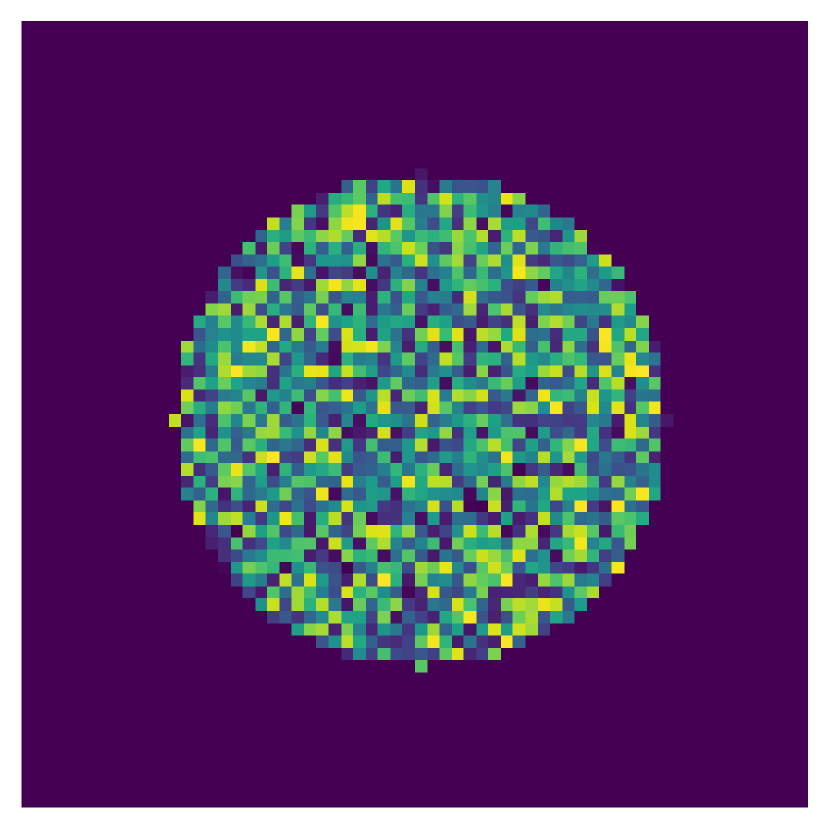
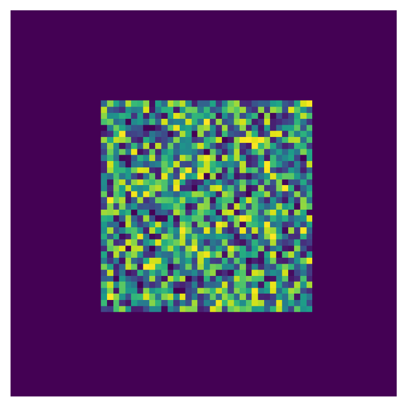
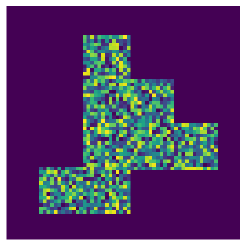
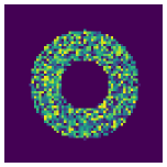
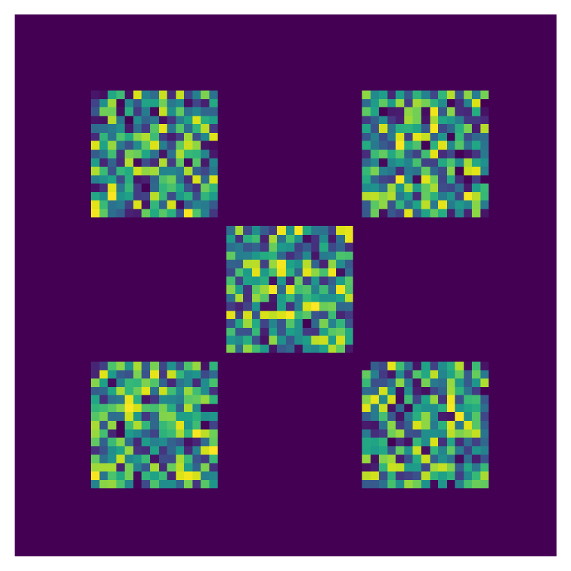
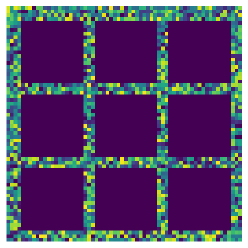
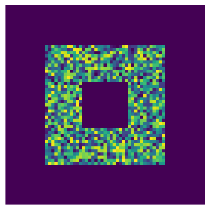
The shapes are the domain of the image pixels with positive intensity. We consider the following shapes: disc, annulus, square, Tetris, clusters, and Swiss cheese; see Fig. 4 for example images of these shapes. When creating these shapes, we ensure that they have approximately the same number of non-zero pixel intensities (of the pixels in the grid); see Table 1.
| Shape | Nonzero Pixels |
|---|---|
| Disc | |
| Square | |
| Tetris | |
| Annulus | |
| Clusters | |
| Swiss Cheese | |
| Square Annulus |
Pixel Intensity.
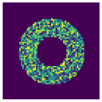
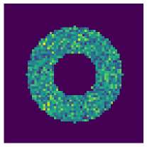
We consider four weight distributions for the pixel intensities: a uniform and three truncated normal distribution with different standard deviations. The uniform distribution takes values greater in the interval , and is denoted . The truncated normal is centered at with a standard deviation of , , and truncated to take values in the interval . The takes three values so that , for , is (approximately) the support, ; in other words, we consider the distributions , , and . Fig. 5 displays the probability densities for these distributions. Notice that as the increases, the distribution of the weights looks more like those of a , and therefore, when doing binary classification, the misclassification rate should increase as is compared to with increasing. Fig. 6 includes an example of an annulus with pixel intensities drawn from a distribution and from a distribution.
Function Extension.
3.2 Classification Methods
The seven shapes, four distributions, and two function extensions define 56 image classes. The WECT is evaluated on the task of binary classification using support vector machines (SVM) [5] and -nearest-neighbors [10]. For each classification model, 250 images (half from each class) are independently generated, with 80 percent of the images (200 images) used for training and the remaining 20 percent (50 images) used for testing. To approximate the WECT, we sample equally-spaced directions from . We discuss results below for choosing different numbers of directions from . To vectorize each WECF, equally-spaced threshold values from to are considered. This ensures that there is at least one discretization value for each height threshold in any direction of filtration.
Implementation.
The simulation study was implemented in Python, using the Dionysus 2 library [16]. For classification tasks using SVM, we train an SVM separately for each binary classification model. All SVMs in this work use a regularization parameter of value 20. The classification was done using an SVM classifier library from Scikit-learn [17]. For classification tasks using -nearest-neighbors, a simple Python implmentation was created using our implementation of the WECT distance function.
3.3 Results
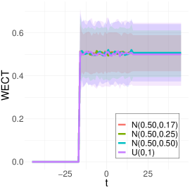
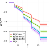
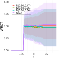
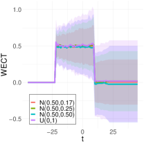
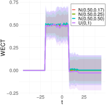
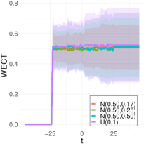
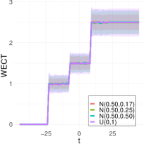
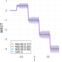
To better understand the WECT, we considered several experiments that provide insight into how different factors affect the WECT and the information it encodes. In particular, we analyze changes in the number of directions, pixel intensity distributions, function extensions, and use of the WECT vs. the vectorized WECT. However, first, as Fig. 7 demonstrates, we verify that for all four pixel intensity distributions, the computation of the WECT matches the theoretical expectation given in Equation (37).
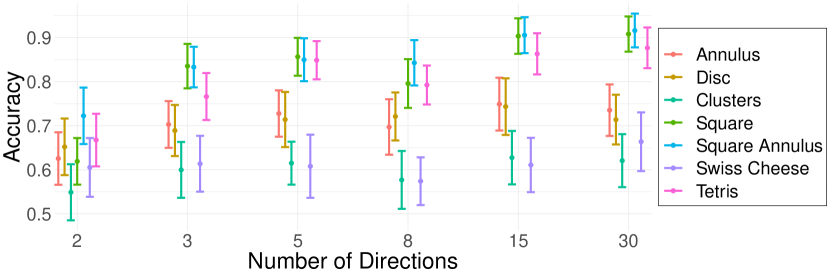
Next, we analyze how changing the number of directions of the filtration impacts the ability of the WECT to capture information about the underlying image. In order to do so, the following classification task was executed using the SVM classifier. For each shape, the image was compared against the in a binary classification task for a varying number of directions. The average function extension was used when computing the WECTs. For a given shape, if the WECT successfully encoded the structure of the two different images, the classification accuracy is closer to one. The classifier accuracy was tested on all the shapes for and directions. As Fig. 8 shows, as the number of directions increases, accuracy of the classifier improved only for some shapes. In order to balance an increase of encoded information in the WECT with computational cost, the remainder of the experiments are executed using 15 directions.
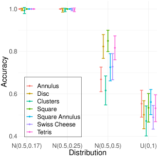
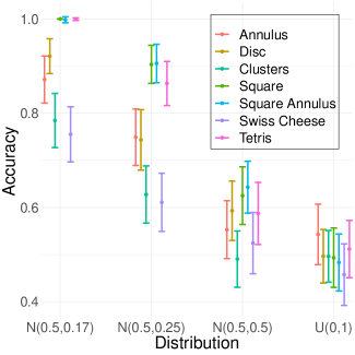
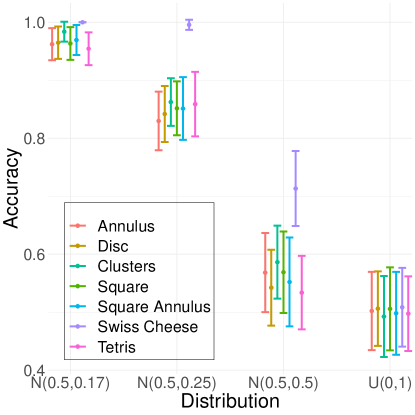
In order to gain a deeper understanding of the WECT properties, we conducted experiments to observe how changing pixel intensity distributions in various filtration directions affect its behavior. Again, we examined the WECT’s capacity to extract image information through binary classification tasks using an SVM classifier. For each shape, we consider the task of binary classification of WECTs in directions from each of the four distributions against the WECT from the distribution. All pairwise classification models were considered, but when image shape differed the classifier performed nearly perfect regardless of the pixel intensity distribution so those results are not summarized further. Results where the two classes have the same shape can be found in Fig. 9 for both function extensions. As anticipated, the accuracy of the classifier for against is roughly random, against is nearly perfect, against is slightly worse, and against is barely better than random. Ultimately, the decrease in accuracy as the normal distribution becomes more similar to the uniform distribution (i.e., as increases) demonstrates that the WECT encodes information about the pixel intensity distribution. In other words, the WECT captures and encodes structural information from the images that is not encoded by the ECT.
Next, we compare the results using the maximum function extension (Fig. 9(a)) and the average function extension (Fig. 9(b)). Overall, across nearly all the distributions, the classifier performs better on WECTs computed using the maximum function extension as opposed to the average function extension. As the distributions differ more at their extremes in the current setting, it is likely that the maximum function extension better emphasizes these differences, which in turn increases the accuracy of the classifier.
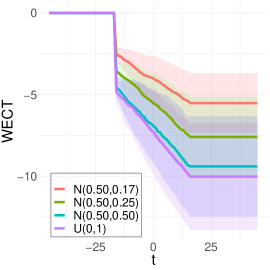
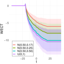
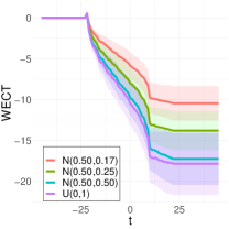
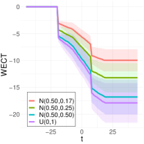
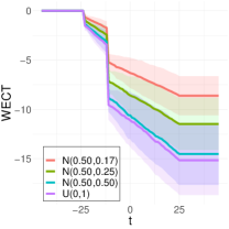
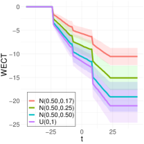
To better understand the classification performance in the above experiments, we consider visualizations of the WECT for the setting that considers fifteen directions. Fig. 10 displays the average WECT in one direction of 250 generated images under the two different function extensions. The shaded region indicates the values within one standard deviation of the mean. For both function extensions, the average WECT generally follows the same pattern, but the values of the WECT depend on the distribution of the pixel intensities. The WECT using the distribution generally has the lowest values, and the WECT using the and distribution tends to have slightly greater values, then , and finally the distribution tends to have the highest values. These results hold also for the rest of the shapes, as indicated in Fig. 11 and Fig. 12. This, along with the classification results, indicate that incorporating the weights into the ECT is important for distinguishing images generated under different intensity distributions. Note also that the average WECT for different shape classes have varying levels and patterns of smoothness, which reveals why the classification rate between different shapes is nearly perfect.
A final result is the use of the true (non-vectorized) WECT in the classification experiments. As explained in Section 2.3, one can compute a distance between two WECTs by integrating the difference between the piecewise WECFs in each direction (and taking the maximum difference across all directions). Thus, a natural extension use of this distance is in a nonparametric classification method such as -nearest-neighbors (KNN). Fig. 13 summarizes results for the KNN classifier based on the WECT distance with for eight directions with the maximum extension. In general, it appears that performance of SVM was better in these binary classification tasks. Extensive experiments with KNN were less feasible due to the high computational cost of nonparametric methods. However, the focus is not on using the WECT as a classifier, but instead using the classification tasks to understand the information that is encoded in the WECT. For both methods, we observe a decrease in accuracy as the pixel intensity distribution becomes more similar, which indicates that both the vectorized WECT and the WECT distance successfully encode underlying information about the image.
4 Conclusion
While the ECT has been successful at summarizing shapes in a variety of contexts, image data poses a unique challenge because the pixel intensities potentially carry significant and relevant information. The WECT was proposed to generalize the ECT and allow for the incorporation of pixel intensities as weights. However, the intuition and interpretation of the WECT is not as clear. In this paper, we explored using the WECT to represent shapes found in images, and developed an understanding of the importance of the weights. Indeed, we found that the WECT captured more than the EC and the ECF alone. This was especially important when images have the same shape, but different intensity distributions as assessed in our empirical study. As the intensity distributions become more similar between two classes that have the same shape, the test classification accuracy decreases. When the two classes had different image shapes, the WECT correctly classified new images perfectly (or almost perfectly with test classification accuracy greater than 0.99). While we limited our classification models to SVM, and explored KNN models, WECTs can be used in other classification models.
The effect on changing inputs to the WECT was also explored. Two function extensions, the maximum and average function extensions, were considered. Though the maximum function extension outperformed the average function extension in our settings, this was likely dependent on the pixel intensity distributions considered. In particular, the four distributions (, , , and ; all truncated to ) had averages of so differences were near the extremes (near zero or one). Therefore, the maximum function extension would amplify these differences better than the average.
We also explored how the test classification accuracy changed with different numbers of directions considered. Shapes with rotational symmetry did not benefit from increasing the number of directions, while those without rotational symmetry did benefit. How to appropriately select the number of directions in this setting is an open question that will be explored in future work.
Though classification was explored in this paper, the WECT could also be used for inference tasks such as hypothesis testing. In light of this, we developed equations for the expected weighted EC and expected WECT for images, which may be useful for developing test statistics in future studies. While we have found a clear benefit in using the WECT for image classification when the pixel intensity distributions differ, questions remain regarding its advantage for inference or for different data types.
References
- [1] P. Alexandroff, Diskrete raume, Mathematiceskii Sbornik, 2 (1937), pp. 501–519.
- [2] E. J. Amézquita, M. Y. Quigley, T. Ophelders, J. B. Landis, D. Koenig, E. Munch, and D. H. Chitwood, Measuring hidden phenotype: Quantifying the shape of barley seeds using the Euler characteristic transform, in silico Plants, 4 (2022), p. diab033.
- [3] E. Berry, Y.-C. Chen, J. Cisewski-Kehe, and B. T. Fasy, Functional summaries of persistence diagrams, Journal of Applied and Computational Topology, 4 (2020), pp. 211–262.
- [4] L. M. Betthauser, Topological reconstruction of grayscale images, PhD thesis, University of Florida, 2018.
- [5] C. Cortes and V. Vapnik, Support-vector networks, Machine learning, 20 (1995), pp. 273–297.
- [6] L. Crawford, A. Monod, A. X. Chen, S. Mukherjee, and R. Rabadán, Predicting clinical outcomes in glioblastoma: an application of topological and functional data analysis, Journal of the American Statistical Association, 115 (2020), pp. 1139–1150.
- [7] H. A. David and H. N. Nagaraja, Order statistics, John Wiley & Sons, 2004.
- [8] T. K. Dey and Y. Wang, Computational Topology for Data Analysis, Cambridge University Press, 2022.
- [9] H. Edelsbrunner and J. Harer, Computational Topology: An Introduction, American Mathematical Soc., 2010.
- [10] E. Fix and J. L. Hodges, Discriminatory analysis. nonparametric discrimination: Consistency properties, International Statistical Review / Revue Internationale de Statistique, 57 (1989), pp. 238–247.
- [11] H. Freudenthal, Simplizialzerlegungen von beschrankter flachheit, Annals of Mathematics, (1942), pp. 580–582.
- [12] R. Ghrist, R. Levanger, and H. Mai, Persistent homology and Euler integral transforms, Journal of Applied and Computational Topology, 2 (2018), pp. 55–60.
- [13] Q. Jiang, S. Kurtek, and T. Needham, The weighted Euler curve transform for shape and image analysis, in Proceedings of the IEEE/CVF Conference on Computer Vision and Pattern Recognition Workshops, 2020, pp. 844–845.
- [14] Y. LeCun, L. Bottou, Y. Bengio, and P. Haffner, Gradient-based learning applied to document recognition, Proceedings of the IEEE, 86 (1998), pp. 2278–2324.
- [15] L. Marsh, F. Y. Zhou, X. Quin, X. Lu, H. M. Byrne, and H. A. Harrington, Detecting temporal shape changes with the euler characteristic transform, 2022. arXiv preprint arXiv:2212.10883.
- [16] D. Morozov, Dionysus 2. https://mrzv.org/software/dionysus2/.
- [17] F. Pedregosa, G. Varoquaux, A. Gramfort, V. Michel, B. Thirion, O. Grisel, M. Blondel, P. Prettenhofer, R. Weiss, V. Dubourg, J. Vanderplas, A. Passos, D. Cournapeau, M. Brucher, M. Perrot, and E. Duchesnay, Scikit-learn: Machine learning in Python, Journal of Machine Learning Research, 12 (2011), pp. 2825–2830.
- [18] K. Turner, S. Mukherjee, and D. M. Boyer, Persistent homology transform for modeling shapes and surfaces, Information and Inference: A Journal of the IMA, 3 (2014), pp. 310–344.
- [19] H. Wagner, C. Chen, and E. Vuçini, Efficient computation of persistent homology for cubical data, in Topological methods in data analysis and visualization II, Springer, 2012, pp. 91–106.