The wobbly Galaxy: kinematics north and south with RAVE red clump giants
Abstract
The RAVE survey, combined with proper motions and distance estimates, can be used to study in detail stellar kinematics in the extended solar neighbourhood (solar suburb). Using red clump stars, we examine the mean velocity components in 3D between and , concentrating on North-South differences. Simple parametric fits to the trends for and the velocity dispersions are presented. We confirm the recently discovered gradient in mean Galactocentric radial velocity, , finding that the gradient is marked below the plane ( for , vanishing to zero above the plane), with a gradient thus also present. The vertical velocity, , also shows clear, large-amplitude () structure, with indications of a rarefaction-compression pattern, suggestive of wave-like behaviour. We perform a rigorous error analysis, tracing sources of both systematic and random errors. We confirm the North-South differences in and along the line-of-sight, with the estimated independent of the proper motions. The complex three-dimensional structure of velocity space presents challenges for future modelling of the Galactic disk, with the Galactic bar, spiral arms and excitation of wave-like structures all probably playing a role.
keywords:
Galaxy: kinematics and dynamics; Galaxy: solar neighbourhood; Galaxy: structure1 Introduction
The more we learn about our Galaxy, the Milky Way, the more we find evidence that it is not in a quiescent, stable state. Rather, the emerging picture is of a Galaxy in flux, evolving under the forces of internal and external interactions. Within the halo, there is debris left by accretion events, the most significant being the Sagittarius stream (Majewski et al., 2003) at a mean distance of associated with the Sagittarius dwarf galaxy (Ibata, Gilmore & Irwin, 1994). In the intersection of halo and disk there are also indications of accretion debris, such as the Aquarius Stream (, Williams et al. 2011) as well as local halo streams such as the Helmi stream (, Helmi et al. 1999). While within the disk itself there is evidence of large-scale stellar over-densities: outward from the Sun at a Galactocentric distance of there is the Monoceros Stream (Newberg et al. 2002, Yanny et al. 2003), inward from the Sun () there is the Hercules thick disk cloud (Larsen & Humphreys 1996, Parker et al. 2003, Parker et al. 2004, Larsen, Humphreys & Cabenela 2008). The origin of all such structures is not yet fully understood: possible agents for the Monoceros ring are tidal debris (see e.g., Penarrubia et al. 2005), the excitation of the disk caused by accretion events (e.g., Kazantzidis et al. 2008) or the Galactic warp (Momany et al. 2006), while Humphreys et al. 2011 conclude that the Hercules cloud is most likely due to a dynamical interaction of the thick disk with the Galaxy’s bar.
Velocity space also exhibits structural complexity. In the solar neighbourhood various structures are observed in the distribution of stars in the plane, which differs significantly from a smooth Schwarzschild distribution (Dehnen, 1998). These features are likely created by the combined effects of the Galactic bar (Raboud et al. 1998, Dehnen 1999, Minchev et al. 2010, Famaey et al. 2007) and spiral arms (De Simone, Wu & Tremaine 2004; Quillen & Minchev 2005, Antoja et al. 2009) or both (Chakrabarty 2007, Quillen et al. 2011). Dissolving open clusters (Skuljan, Cottrell & Hearnshaw 1997, De Silva et al. 2007) can also contribute to structure in the plane. Finally, velocity streams in the plane can be explained by the perturbative effect on the disk by recent merger events (Minchev et al. 2009, Gomez et al. 2012).
Venturing beyond the solar neighbourhood into the solar suburb, Antoja et al. 2012 used data from the RAdial Velocity Experiment (RAVE) (Steinmetz et al., 2006) to show how these resonant features could be traced far from the Sun, up to from the Sun in the direction of anti-rotation and below the Galactic plane. Additionally, Siebert et al. 2011 (hereafter S11), showed based on RAVE data that the components of stellar velocities in the direction of the Galactic centre, , is systematically non-zero and has a non-zero gradient . A similar effect was seen in the analysis of 4400 RAVE red clump giants by Casetti et al. 2011. The cause of this streaming motion has been variously ascribed to the bar, spiral arms, and the warp in conjunction with a triaxial dark-matter halo, or a combination of all three. Recently, Siebert et al. 2012 have used density-wave models to explore the possibility that spiral arms cause the radial streaming, and were able to reproduce the gradient with a two-dimensional model in which the Sun lies close to the 4:1 ultra-harmonic resonance of two-arm spiral, in agreement with Quillen & Minchev 2005 and Pompéia et al. 2011. While structure in the plane smears out with the increase of sample depth (at ), Gomez et al. (2012a,b) showed that energy-angular momentum space preserves structure associated with “ringing” of the disk in response to a minor merger event for distances around the Sun as large as , consistent with the SEGUE and RAVE coverage.
In this paper we examine the kinematics of the red clump giants in the three-dimensional volume surveyed by RAVE, focusing particularly on differences between the northern and southern sides of the plane. The full space velocities are calculated from RAVE line-of-sight velocities (), literature proper motions and photometric distances from the red clump. We have sufficient stars from the RAVE internal data set for the stellar velocity field to be explored within the region and . While studies such as Pasetto et al. 2012a, b, distinguish between thick- and thin-disk stars, we do not. Distinguishing between the thin, thick disk and halo require either kinematic or chemical criteria, each of which have their individual issues and challenges, which we wish to avoid. Rather, our aim here is to describe the overall velocity structure of the solar neighbourhood in a pure observational/phenomenological sense. The interpretation of this based on thin or thick-disk behaviour is then secondary.
In S11, as a function of was examined. Here we extend this analysis to investigate particularly the dependence of , as well as the other two velocity components, and , with a simple parametric fit for presented. We find that the average values of and show a strong dependence on three-dimensional position. We compare these results to predictions of a steady-state, axisymmetric Galaxy from the Galaxia (Sharma et al., 2011) code. To visualise the 3D behaviour better, various projections are used. Further, the detection by S11 of the gradient in using only line-of-sight velocities is re-examined in light of the results seen in 3D, extending the analysis to include . As an aside, parametric fits to the velocity dispersions are presented.
The paper also includes a thorough investigation into the effects of systematic and measurement errors, which almost everywhere dominate Poisson noise. The assumptions used to calculate photometric distances from the red clump are examined in some detail, where we model the clump using Galaxia. The effects of using alternative sources of proper motion are shown in comparison with the main results, as we found this to be one of the largest systematic error sources.
The paper is organised as follows. In Section 2 we discuss our overall approach for the kinematic mapping, the co-ordinate systems used and initial selection from RAVE. In Section 3 we present a detailed investigation into the use of the red clump stars as a distance indicator, where we introduce a Galaxia model of the red clump to model the distance systematics. In Section 4 we present our error analysis, investigating systematic error sources first before discussing measurement errors, Poisson noise and the final cuts to the data using the error values. In Section 5 we examine the 3D spatial distribution of our data before going on in Section 6 to investigate the variation for and over this space. Also presented are the variations in velocity dispersions with and a simple functional fit to these trends. In Section 7 we use the line-of-sight method to investigate the and trends towards and away from the Galactic centre, while finally, Section 8 contains a summary of our results.
2 Red Clump kinematics with RAVE data
2.1 Co-ordinate systems and Galactic parameters
As we are working at large distances from the solar position, we use cylindrical co-ordinates for the most part, with and defined as positive with increasing , and , with the latter towards the North Galactic Pole (NGP). We also use a right-handed Cartesian co-ordinate system with increasing towards the Galactic centre, in the direction of rotation and again positive towards the NGP. The Galactic centre is located at . Space velocities, , are defined in this system, with positive towards the Galactic centre.
To aid comparison with the predictions of Galaxia (see Section 2.3), we use mostly the parameter values that were used to make the model for which Galaxia makes predictions. Thus, the motion of the Sun with respect to the LSR is taken from Schönrich, Binney & Dehnen 2010, namely . The LSR is assumed to be on a circular orbit with circular velocity . Finally, we take . The only deviation from Galaxia’s values is that they assumed that the Sun is located at , while we assume .
S11 explored the variation of the observed gradient on the values of and , finding that changing these parameters between variously accepted values could reduce but not eliminate the observed gradient in . We do not explore this in detail in this paper but note that the trends that we observe are similarly affected by the Galactic parameters; amplitudes are changed but the qualitative trends remain the same.
2.2 RAVE data
The wide-field RAVE (RAdial Velocity Experiment) survey measures primarily line-of-sight velocities and additionally stellar parameters, metallicities and abundance ratios of stars in the solar neighbourhood (Steinmetz et al., 2006; Zwitter et al., 2008; Siebert et al., 2011; Boeche et al., 2011). RAVE’s input catalog is magnitude limited () and thus creates a sample with no kinematic biases. To the end of 2012 RAVE had collected more than 550,000 spectra with a median error of (Siebert et al., 2011b).
| Version | Source | |
|---|---|---|
| A | Observation: Alves 2000, Grocholski & Sarajedini 2002 | |
| B | Observation: Groenewegen 2008 | |
| C | Theory: Salaris & Girardi 2002 compared to the RAVE population |
We use the internal release of RAVE from October 2011 which contains 434,807 RVs and utilizes the revised stellar parameter determination (see the DR3 paper, Siebert et al. 2011b for details). We applied a series of cuts to the data. Firstly, those stars flagged by the Matijevič et al. 2012 automated spectra classification code as having peculiar spectra were excluded. This removes most spectroscopic binaries, chromospherically active and carbon stars, spectra with continuum abnormalities and other unusual spectra. Further cuts restricted our sample to stars with signal-to-noise ratio (STN is calculated from the observed spectrum alone with residuals from smoothing, see Section 2.2 of the DR3), Tonry & Davis 1979 cross-correlation coefficient , , , (see Section 4.4) and stars whose SpectraQualityFLAG is null. Where there are repeat observations, we randomly select one observation for each star. With this cleaning, the data set has 293,273 unique stars with stellar parameters from which to select the red clump.
In some fields at the RAVE selection function includes a colour cut with the object of favouring giants. We imposed this colour cut throughout this region to facilitate the comparison to predictions by Galaxia. The selection of red clump stars is unaffected by this cut. Additional data cuts and selections were performed later in the analysis and are broadly a) the selection of red-clump giants (Section 3.3), b) removal of stars with large extinction/reddening (Section 4.1.5), and removal of data bins with large errors in measurements of mean velocity (Section 4.4).
As a sample with alternative distance determinations, we also used an internal release with stellar parameters produced by the pipeline that was used for the third Data Release (VDR3) and the method of Zwitter et al. 2008 from September 2011 with 334,409 objects. We cleaned the sample as above, leaving us with 301,298 stars.
A newer analysis of RAVE data is presented in the 4th RAVE data release, Kordopatis et al. (in preparation). This applies an updated version of the Kordopatis et al. 2011 pipeline to RAVE spectra. Selecting red clump stars using the stellar parameters from this pipeline does not produce significantly different results to those selected using the VDR3 pipeline above; the conclusions of this paper are unaffected by the pipeline used for the red-clump selection.
2.3 The Galaxia model
In Williams et al. 2011 we introduced the use of the Galaxy modelling code Galaxia (Sharma et al., 2011) to investigate the statistical significance of the new Aquarius stream found with RAVE. In this study we use Galaxia both to provide predictions with which to compare our results, and to investigate the effects of contamination of the red-clump sample by stars that are making their first ascent of the giant branch (see Section 4.1.1). Galaxia enables us to disentangle real effects from artifacts of our methodology, and further to understand the population we are examining.
Based on the Besançon Galaxy model, the Galaxia code creates a synthetic catalog of stars for a given model of the Milky Way. It offers several improvements over the Besançon model which increase its utility in modelling a large-scale survey like RAVE, the most significant of which is the ability to create a continuous distribution across the sky instead of discrete sample points. The elements of the Galactic model are a star formation rate, age-velocity relation, initial mass function and density profiles of the Galactic components (thin and thick disk, smooth spheroid, bulge and dark halo). The parameters and functional forms of these components are summarized in Table 1 of Sharma et al. 2011.
We follow a similar methodology to that described in Williams et al. 2011 to generate a Galaxia model of the RAVE sample, from which we select a red clump sample following the selection criteria applied to the real data. A full catalog was generated over the area specified by , and , with no under-sampling. As described in Section 3.2, the RAVE data were then divided into three signal-to-noise regimes and a sample drawn from the Galaxia model so that, for each regime, the -band distribution was matched to that of the RAVE sample in squares. The Galaxia -band was generated after correcting for extinction.
3 The Red Clump
The helium-burning intermediate-age red clump has long been seen as a promising standard candle (Cannon et al., 1970), with its ease of identification on the HR diagram. In recent years there has been a renewed interest in the red clump for distance determination, e.g., Pietrzyński, Gieren & Udalski 2003 studied the clump in the Local Group, down to the metal-poor Fornax dwarf galaxy. Here we investigate the use, selection and modelling of this population in solar-suburb RAVE data.
3.1 The Red Clump -band magnitude
The -band magnitude of the red clump, while being relatively unaffected by extinction, has also been shown observationally to be only weakly dependent on metallicity and age (Pietrzyński, Gieren & Udalski, 2003; Alves, 2000), so a single magnitude is usually assigned for all stars in the red clump. Studies such as Grocholski & Sarajedini 2002 and van Helshoecht & Groenewegen 2007 have shown that there is some dependence on metallicity and age which can be accounted for by the theoretical model of Salaris & Girardi 2002.
If models correctly predict the systematic dependence of of the red clump on metallicity and age, this would have implications for our study of kinematics in the solar suburb, for with increasing distance above the plane the metallicity will decrease and the population become older. From Burnett et al. 2011 we estimate that the population means change from , at to , at . According to Salaris & Girardi 2002, these age and metallicity changes will change the -band absolute magnitude from 111Here is used to denote -band magnitudes in the Bessell & Brett 1989 system, while is used to denote 2MASS values. The relations from Carpenter 2003 were used to convert between the two photometric systems. Note though that is shortened to in Section 3.2 and beyond. at to at . Hence, the distances to stars at higher will be systematically underestimated by .
Furthermore, there is uncertainty regarding the average value of . Alves 2000 gives for local red clump giants with Hipparcos distances and metallicities between . In the 2MASS system the corresponding absolute magnitude is . Grocholski & Sarajedini 2002 derives a similar value of for , from 2MASS data of open clusters. Extending the sample of clusters, van Helshoecht & Groenewegen 2007 derived for , . Then using the new van Leeuwen 2007 Hipparcos parallaxes, Groenewegen 2008 found that the Hipparcos red clump giants now give () over , with a selection bias, whereby accurate K-magnitudes are only available for relatively few bright stars, meaning the actual value is likely brighter. The newer values hold better agreement with the theoretical results of Salaris & Girardi 2002, who derived an average value for the solar neighbourhood of , derived via modelling with a SFR and age-metallicity relation.
Given the disagreement over the -band magnitude for the clump and possible metallicity/age variations, we investigated the use of the three normalizations for for our derivation of the RAVE red clump distances. Table 1 summarizes these values, where the Version A is the standard value from Alves 2000 and Grocholski & Sarajedini 2002, while Version B is the new value from Groenewegen 2008. Version C is derived from the theoretical models of Salaris & Girardi 2002 and attempts to take into account some of the possible systematics for lower metallicity stars, where we use the variation of age and metallicity of RAVE stars described above (i.e., at to at ) to develop a simple linear relation of with , where the value for each star is derived iteratively. In Section 4.1.2 we examine the effect of the different normalizations on our results.
3.2 The Galaxia red clump
To establish the best selection method for the red-clump stars we first tried to match the observed distribution of the selected RC stars with the prediction of Galaxia. The errors in RAVE stellar parameters decrease with STN, so the red clump is more localized at higher STN values. Further, the errors in and are correlated. To account for this in the modelling of the clump, we split the data into three regimes: STN values between , and . We then generated Galaxia models for each STN regime for squares, matching the I-band distribution of Galaxia to that of RAVE in bins of 0.2 mag. The three models for each STN slice of the data were added together to give an overall Galaxia model, with an STN value of 20, 40 or 60 assigned to the Galaxia ‘stars’ to indicate which STN regime they were generated from. Note that, as stated in the DR2 and DR3 releases, the DENIS I-band photometry has large errors for a significant fraction of the stars. We therefore used Equation 24 from the DR2 paper to calculate I magnitudes for those RAVE stars which do not satisfy the condition , as well as those that have 2MASS photometry but no DENIS values. For the models the reddening at infinity is matched to that of the value in Schlegel map and to convert to extinction in different photometric bands we used the conversion factors in Table 6 of Schlegel et al. 1998.
Errors were then added to the values of , and from Galaxia to match the distributions in the RAVE data. The same seed was used for the random number generator for the temperature and gravity values to account for the error covariance. Table 2 gives the standard deviations of the errors that were added to the values from Galaxia. The average error, , is smaller than the expected average observational error in , . An error of in corresponds to an error in of (Alonso, Arribas & Martinez-Roger, 1996). Given this small value and that, unlike , the spread in does not change with STN, we opted to select the RAVE red clump in .
3.3 Selection of RC stars
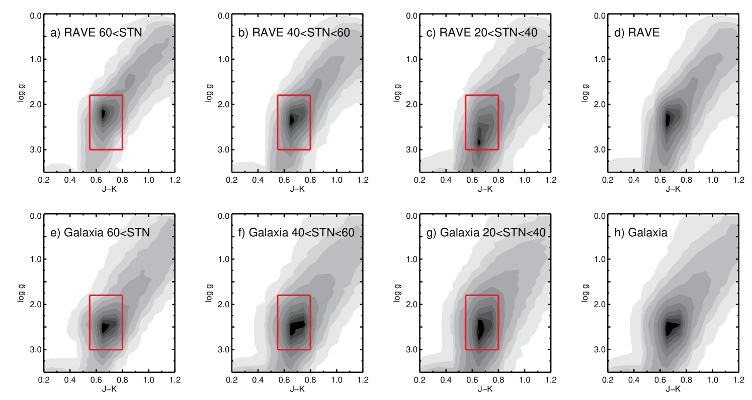
Figure 1 plots the plane for the RAVE giants within in the three STN regimes along with the corresponding Galaxia predictions including errors. Here we see the clump at and . There are some notable differences between the models and the observed distributions. First, the position of the clump in decreases with decreasing STN for the RAVE stars. This change is not matched by Galaxia: the predicted distribution has mean . With increasing dispersion at lower STN it elongates but does not shift. Thus, the effect seen in the RAVE data appears not to be astrophysical in origin but rather a result of the parameter determination from RAVE spectra (for a discussion on systematic trends of stellar parameter estimates with SNR see DR3). Also, there is an absence of horizontal-branch stars below in the RAVE data relative to the prediction by Galaxia. This latter difference does not affect our results as they are not included in the selection region.
| STN regime | |||
|---|---|---|---|
| 0.25 | 25 | 0.01 | |
| 0.35 | 110 | 0.01 | |
| 0.45 | 150 | 0.01 |
We select the red clump as those stars within , . We do not include a STN dependence as extending the selection box further up in gravity will mean an increased fraction of sub-giants in the sample and thus erroneous distances. The red box in Figure 1 displays the selection criteria, where we see that for some of the clump is cutoff at higher values of . Applied to our entire cleaned RAVE set, this selection yields 78,019 stars. A sample of red clump stars were also selected from the Galaxia model in the same way, with a slightly smaller number of 73,594 ‘stars’.
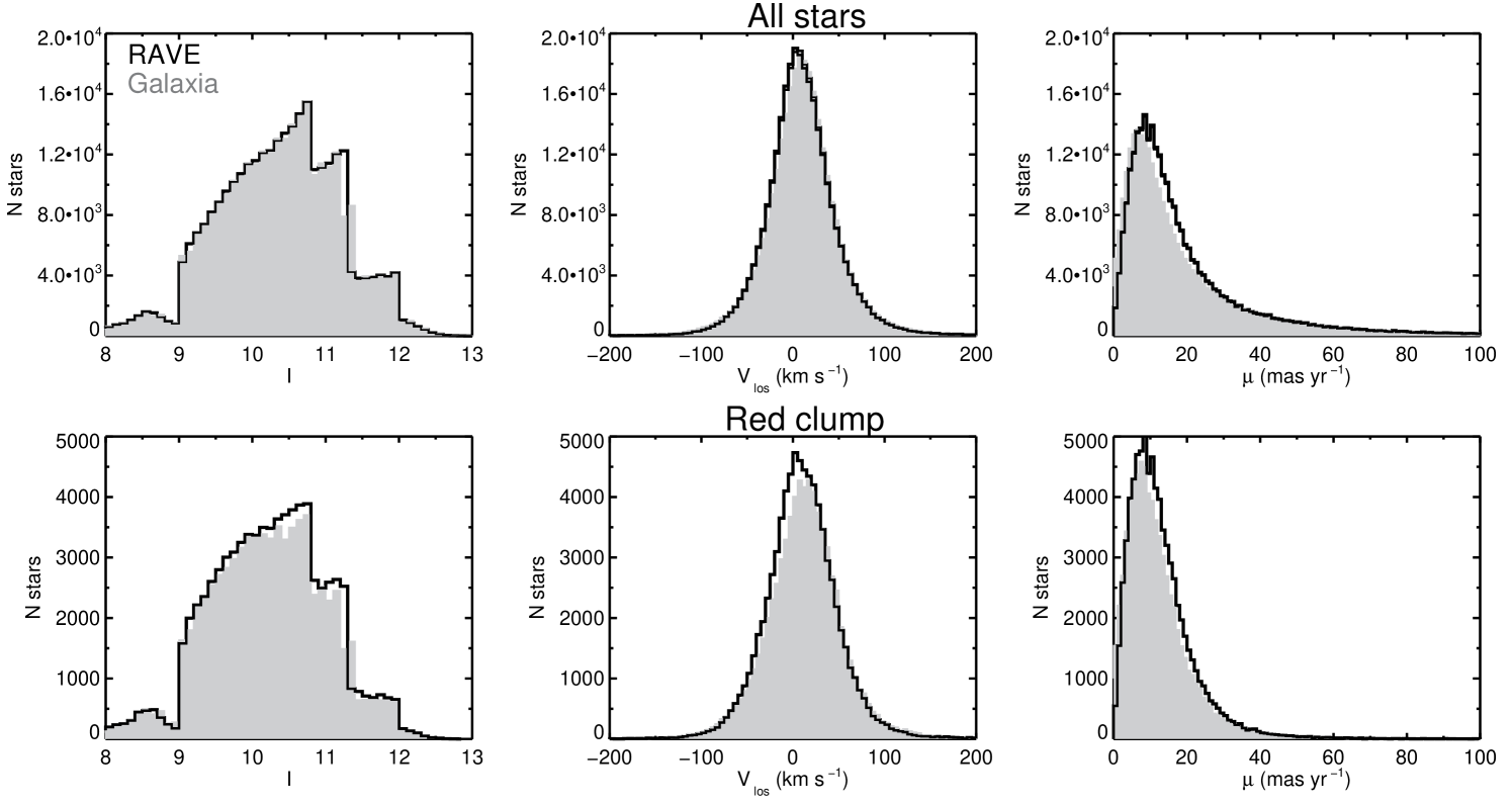
Figure 2 gives the distributions of the entire RAVE data set and red clump stars in and overall proper motion, . The distributions from Galaxia are also given, with an additional spread of and added to the Galaxia line-of-sight velocity and proper motion, respectively, to simulate the observational uncertainties. These values give the average value of the error in these quantities for the RAVE catalog stars. Here we see that Galaxia reproduces quite well the basic distributions of the two observational kinematic parameters which affirms our use of it in comparisons. The small difference in the proper motion distribution could suggest that the actual errors in proper motion are slightly larger than estimated.
4 Error analysis
The most problematic errors are systematic ones. There are multiple ways that these can be introduced into the kinematics. We examine these in some detail before discussing measurement errors in Section 4.2, Poisson noise in Section 4.3 and the final data cuts in Section 4.4.
4.1 Systematic error sources
4.1.1 Contamination by first-ascent giants
In the plane the red clump is overlaid on the first-ascent giant branch (see Figure 1). Our selection criteria therefore also select first-ascent giants, including some sub-giants, which can lead to distance and velocity errors. To assess how this contamination affects our distances and kinematics, we use the red-clump selected stars from the Galaxia model and compute a distance to them assuming a single red-clump magnitude. These results can then be compared to the true values for the model stars. Galaxia uses mainly Padova isochrones and with a median red-clump K-band magnitude of . This is slightly different to that applied above to our data, but is not significant as we are only performing an internal comparison with Galaxia.
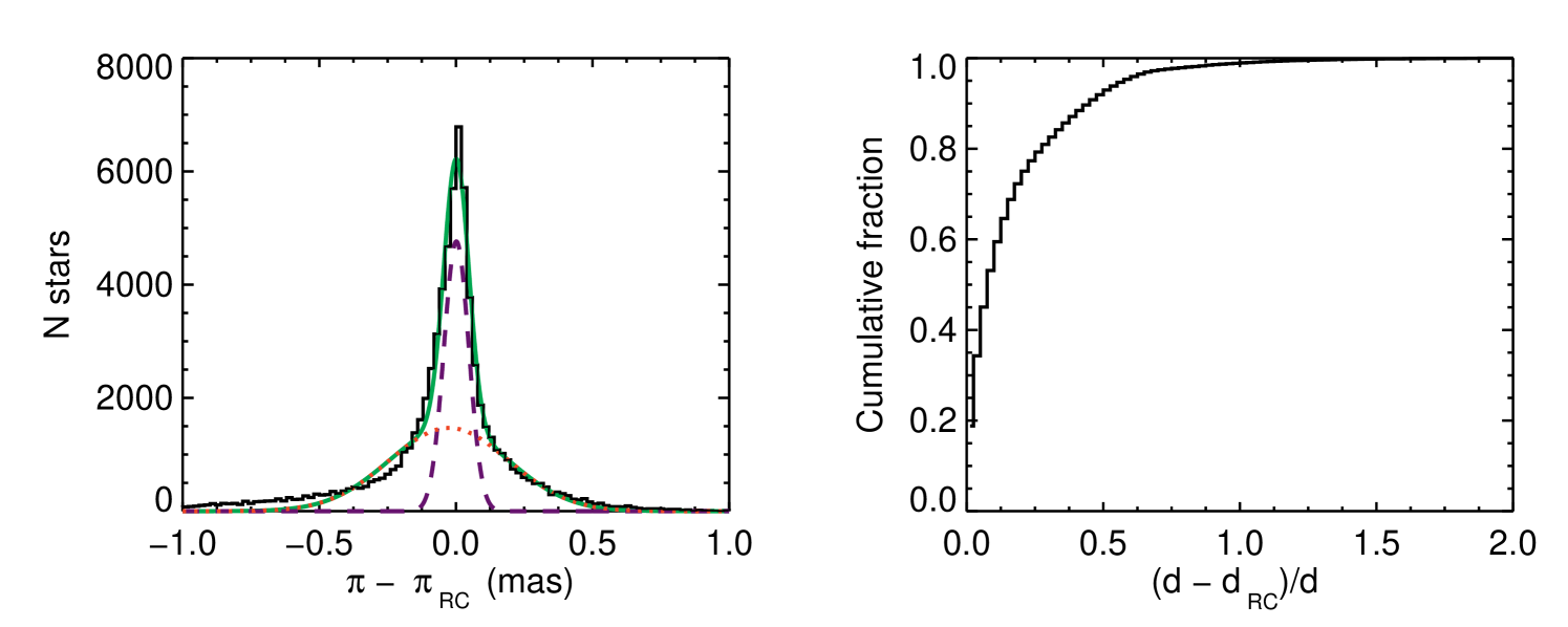
Figure 3a shows the histogram of the parallax errors. The distributions can be decomposed into two Gaussians; one representing the red clump and the other first-ascent giants. Note that the histogram of distance errors does not have such a tidy Gaussian decomposition, hence why we work with the parallax errors. The spread in the red-clump values is caused by the clump’s distribution in age and metallicity; the average value chosen is not true for all red-clump stars. The first-ascent giants have larger errors because while their values may overlap with the clump, their absolute -band magnitude can be quite different. From this decomposition we estimate that the of selected stars are actually red-clump stars and the rest are first-ascent giants. Fortunately however, the mean of the background distribution is very similar to that of the red clump, with a systematic shift of only in distance. In Figure 3b we plot the cumulative distribution of the distance errors. From this we can see that despite the high level of contamination, of stars have distances errors of less that .
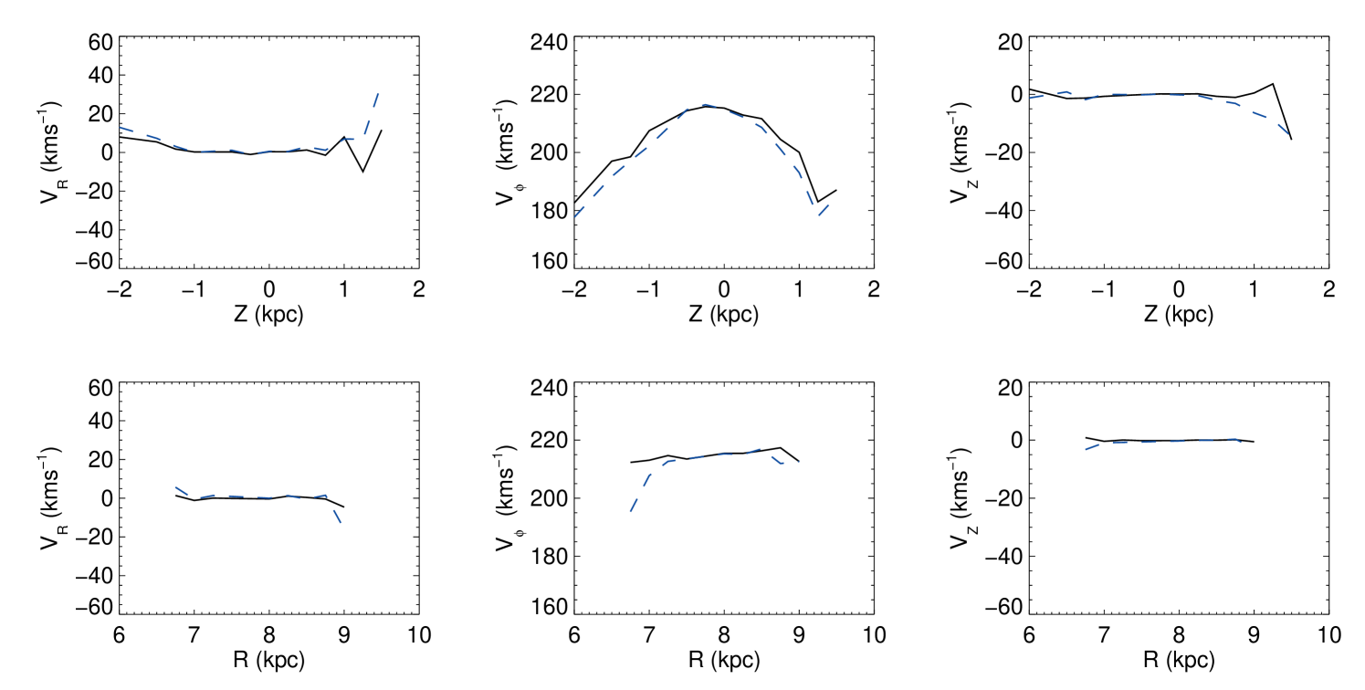
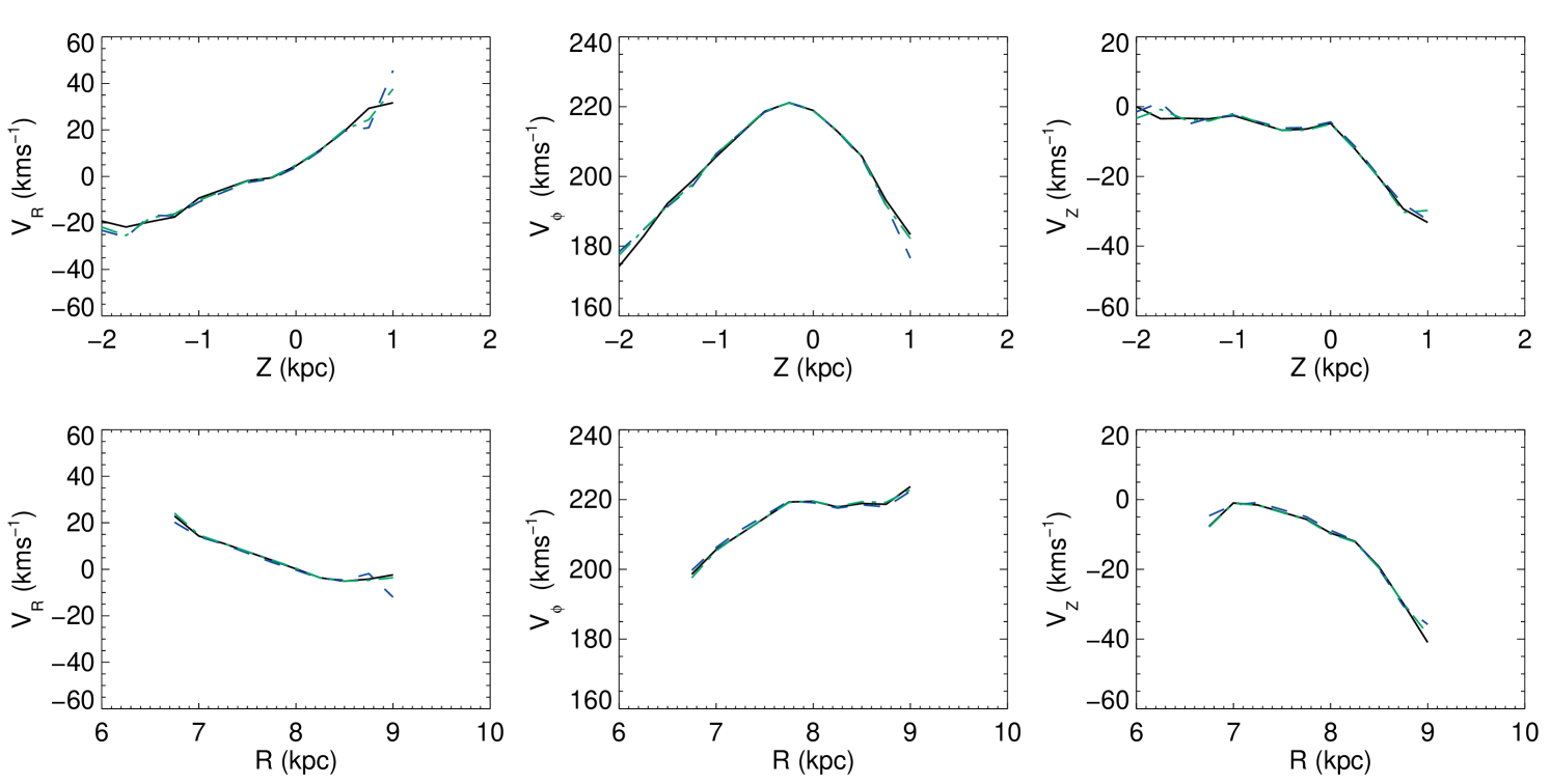
To establish just how these distance errors affect our results, we calculated for stars in the solar cylinder () from the pseudo-data produced by Galaxia using both the true distance to each star, and the distance one infers from the star’s apparent magnitude and a single RC . The upper panels of Figure 4 show the resulting plots of mean velocity components as a function of . In the panels for and the differences between the velocities from true distances (solid line) and from ones derived from a single absolute magnitude (dashed line) are noticeable only at the limits of the surveyed region. In the case of the single value of leads to a consistent underestimation by . The lower panels of Figure 4 show the corresponding results for stars that lie within of the plane, binned in . Again the impact on and of using a single absolute magnitude is evident only at the survey limits. We conclude that the use of a single value of does not significantly compromise our results.
4.1.2 normalisation
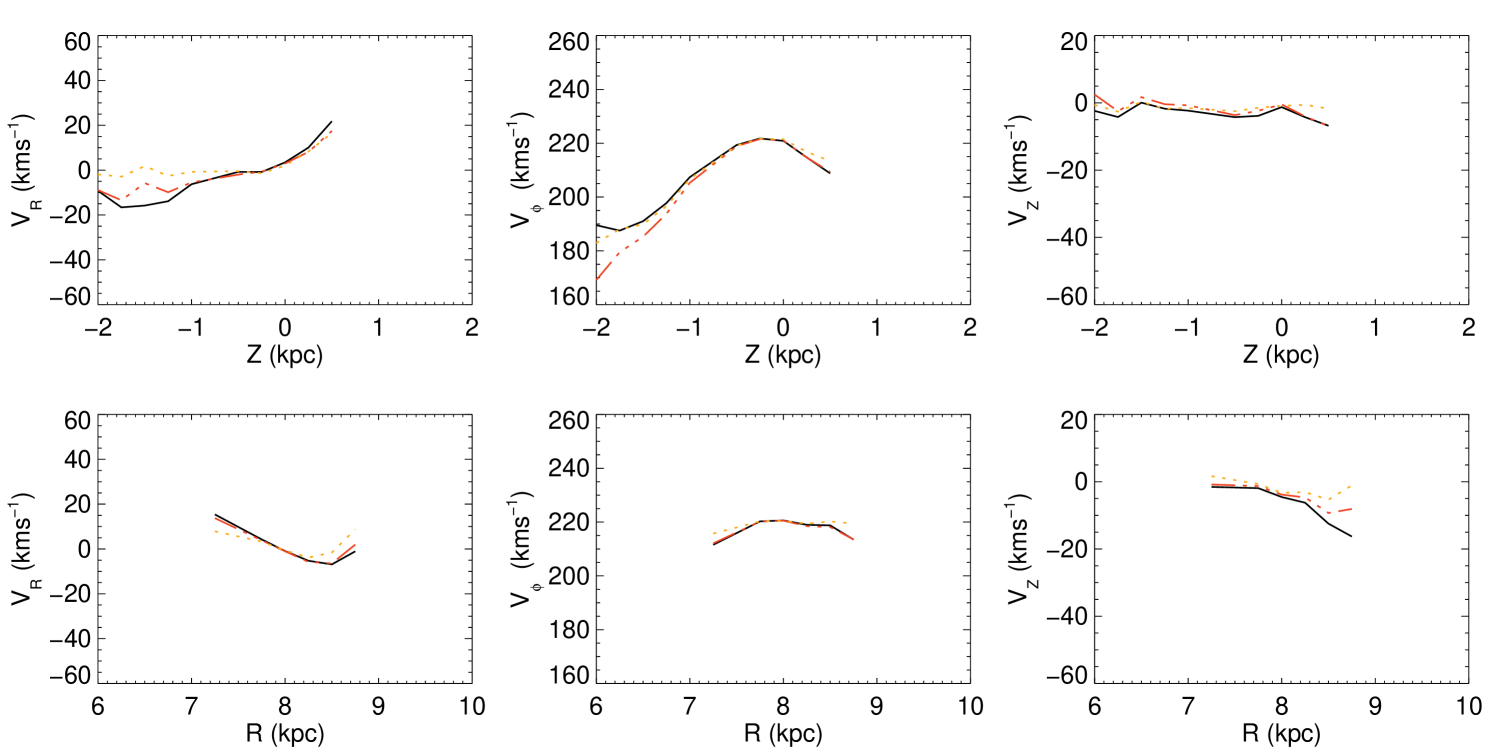
In Section 3.1 we introduced three different normalizations for the value for the red clump. Figure 5 shows the effect of using these different normalizations on the average values of for stars in the solar cylinder (top row of panels) and for stars within of the plane (lower row). We see that the differences in distance produced by the three normalizations has an insignificant impact on the average velocities: only at the limits of the survey, where sample sizes are small, do the differences reach . Thus the dispersion in the velocity errors, on the order of , caused by the single assumption are averaged over and thus all but vanish. It is only those bins - the farthest ones - with the lower number of stars that show any effect.
Given that the effect of the absolute-magnitude normalisation is minor, we use only normalization A for the remainder of this analysis.
4.1.3 Proper motions
RAVE proper motions are derived from several sources, although the majority of the catalog gives PPMX (Roeser et al., 2008) or UCAC2 (Zacharias et al., 2004) proper motions. To investigate the contribution of systematic proper-motion errors, we cross-matched with two additional proper-motion catalogs, the third US Naval Observatory CCD Astrograph Catalog, UCAC3 (Zacharias et al., 2010), and the Yale/San Juan Southern Proper Motion Catalog, SPM4 (Girard et al., 2011). The UCAC3 proper motions suffer from strong plate-dependent systematic distortions north of (Roeser et al., 2010), and so we exclude stars with in this catalog.
Figure 6 shows the mean values of , and with and for stars below calculated using the three sources of proper motions, where the restrictions in and were made to keep as uniform as possible the fractions of stars that have entries in each of the three catalogs. The mean velocities do change with proper-motion source, with the discrepancies largest between RAVE proper motions and those from the SPM4 catalog. The divergence is largest for for and with differences up to in . Some of these variations may be the result of different coverage of the sample volume – which we have tried to minimize with the restrictions on above. Nevertheless, it does indicate that the proper motions are a significant source of systematic error.
It is difficult to say a priori which catalog is closer to the truth; a detailed comparison is beyond the scope of this paper. Given that the systematic differences between proper-motion catalogs can cause significant differences in the derived velocities, we use all three proper motion catalogs in our further analysis, concentrating on the two most divergent proper motions, namely those in the RAVE and SPM4 catalogs.
4.1.4 Binary stars
Two types of spectroscopic binaries can potentially affect our results; single-lined spectroscopic binaries (SB1) stars and double-lined spectroscopic binaries (SB2) stars. Both kinds introduced an additional velocity variation to the sample, with the magnitude much larger for SB2 stars. For the SB2 stars, there is the additional problem that the RAVE processing pipeline assumes that each observed spectrum is that of a single star.
Matijevič et al. 2011 uses repeat observations to estimate the fraction of single-line spectroscopic (SB1) binary stars in the RAVE sample, finding a lower limit of of the sample consists of SB1 stars. The technique is biased towards shorter period binaries, but can be used to gauge the contribution to the measured dispersions from SB1 stars. In Matijevič et al. 2011 the mode of the distribution in the velocity variation from the SB1 stars is . Undetected, long period binary stars will have smaller velocity variations. Thus, the small additional velocity dispersion on a limited fraction of the red clump stars from SB1 sources can be neglected, especially as we are measuring mean velocities in this paper. The fraction of SB2 stars in RAVE is much smaller; Matijevič et al. 2010 estimates of the sample are SB2 stars. Many of these are flagged however, as well as any other peculiar stars, and have been removed from the sample. Unresolved SB2 stars are fortunately rare (Matijevič et al., 2010) and these and the remaining SB2 stars do not affect our results substantially.
4.1.5 Extinction correction
As in Williams et al. 2011, extinction is calculated iteratively from the distances using Schlegel et al. 1998 dust maps and assuming a Galactic dust distribution as in Beers et al. 2000. Note that the maps were adjusted using the correction of Yasuda, Fukugita & Schneider 2007. The extinction reaches relatively large values of for . However, the effect on the velocities is minor; the effect of the extinction correction on the total space velocity is greater than in only of red clump stars. These stars were excluded from further analysis, leaving 72,365 stars in our red clump sample.
4.2 Measurement errors
The non-systematic sources of errors in the kinematics can be broadly broken into (i) the contribution of random uncertainties in the measurements and (ii) the finite sample size for each volume bin. We will examine each of these in turn, before discussing any kinematic cuts that were applied to the data.
The Monte Carlo method of error propagation enables an easy tracking of error covariances, so we employ it here by generating a distribution of 100 test particles around each input value of distance, proper motion, line-of-sight velocity222The positions of the stars are assumed to have negligible errors. and then calculating the resulting points in . We assume that the proper motions and line-of-sight velocities have Gaussian errors with standard deviations given by the formal errors for each star. For the distribution in distance for each star however, we generate a double-Gaussian distribution in the parallax as in Figure 3, which we then invert to derive the distance distribution. This takes into account the fact that errors in distance are due both to the intrinsic width of the RC and the mis-classification of other giants. The ratio between the RC and first-ascent giants for Galaxia model stars changes with distance, where we found a smaller amount of contaminants for . The double-Gaussian in parallax then has dispersions at a ratio of for and for .
4.3 Poisson noise
In each of the bins that are used to calculate the mean velocities, there are a finite number of stars , so Poisson noise contributes to the errors in the derived kinematic properties. These errors scale as . To establish the error contribution from this source we used Bootstrap case resampling with replacement: for each kinematic quantity we derived a distribution in the values by randomly resampling from the distribution of values in the bin. The variance in each value could then be calculated from the resulting distribution. Poisson errors can dominate over measurement errors in bins at large distances that contain very few stars.
To ensure that Poisson errors do not dominate our plots, we only use bins which have and only include those points that have errors in the mean of less than (see Section 4.4).
4.4 Data cuts
There are several ways in which to prune the data to those that are deemed more reliable. However, pruning is liable to introduce kinematic biases. We investigated the effects on the measured velocities of trimming data via a) proper motion, b) error in proper motion, c) distance errors, d) magnitude of total velocity and e) total velocity error, . In general, we found that as we increase the cut-off point there is a steady increase in velocity dispersion and fluctuations in the average velocity, asymptotically approaching a value as the number of stars approaches the full sample. It is therefore difficult to justify cuts that remove a significant proportion of stars. We therefore introduced cuts that remove only the outlier values, as given in Table 3, and we do not perform a cut on .
| Cut | Reason |
|---|---|
| Remove outlier velocities | |
| Remove outlier velocities | |
| Remove outlier proper motions | |
| Remove high proper motion stars | |
| Zwitter only, remove large distance error stars |
Since we seek only to follow trends with , we do not distinguish between halo, thick and thin disk stars. The cuts in total velocity therefore aim to be inclusive of halo stars; the limit is the halo dispersion of (Vallenari et al., 2006). An additional cut in is also introduced to limit ourselves to stars that have plausible rotation velocities.
In our analysis we bin the data in physical space, calculating the means and dispersion in each bin. A further data cut was performed post-binning. For each bin we calculate the mean . For each of these we also calculate an error in the mean, given by standard error propagation as
| (1) |
where and , with the number of stars in the average. The values are given by the MC propagation described in Section 4.2. We remove bins with large errors, i.e., . This affects only peripheral points at large distances from the Sun.
5 Spatial distribution
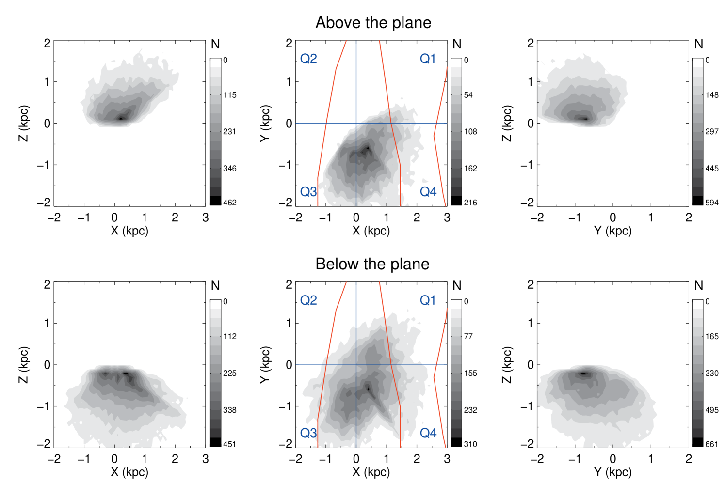
Before examining the velocity trends it is helpful to examine the spatial distribution, to see which regions the RAVE red clump selection function samples. Figure 7 gives the distribution for the RAVE red clump stars, where we have differentiated between stars above and below the plane for clarity. Due to RAVE’s magnitude limit, the red clump stars sample a region between . This, combined with RAVE’s uneven sky coverage between the Northern and Southern Galactic hemispheres, means that the sample region is mostly outside and Quadrants 1 and 2 above the plane are not sampled.
As in S11, S12, we also plot the location of the spiral arms as inferred from the CO maps of Englmaier, Pohl and Bissantz 2008. Going from outer to inner (left to right), the arms are the Perseus, Sagittarius-Carina and Scutum-Centurus arms. We see that our sample misses the Scutum-Centurus arms entirely, and samples above and below the other two spiral arms.
Another significant nearby feature is the Hercules thick-disk cloud (HTDC) (Larsen & Humphreys 1996, Parker et al. 2003. Parker et al. 2003 detected it via star counts in the region both above and below the plane at latitudes . This is in Quadrant 1. Recently, Larsen, Cabenela & Humphreys 2011 reported that the HTDC starts at in our co-ordinates, for . From Figure 7 we can see that the RAVE sample in the south intersects with this location of the Hercules thick-disk cloud. Jurić et al. 2008 also found the HTDC in the location , corresponding to in our co-ordiantes. This region is not covered by the RAVE survey so we cannot see the northern component of the HTDC. In the same paper, another stellar over-density was found at (), which is just missed by the RAVE volume.
6 Velocity trends
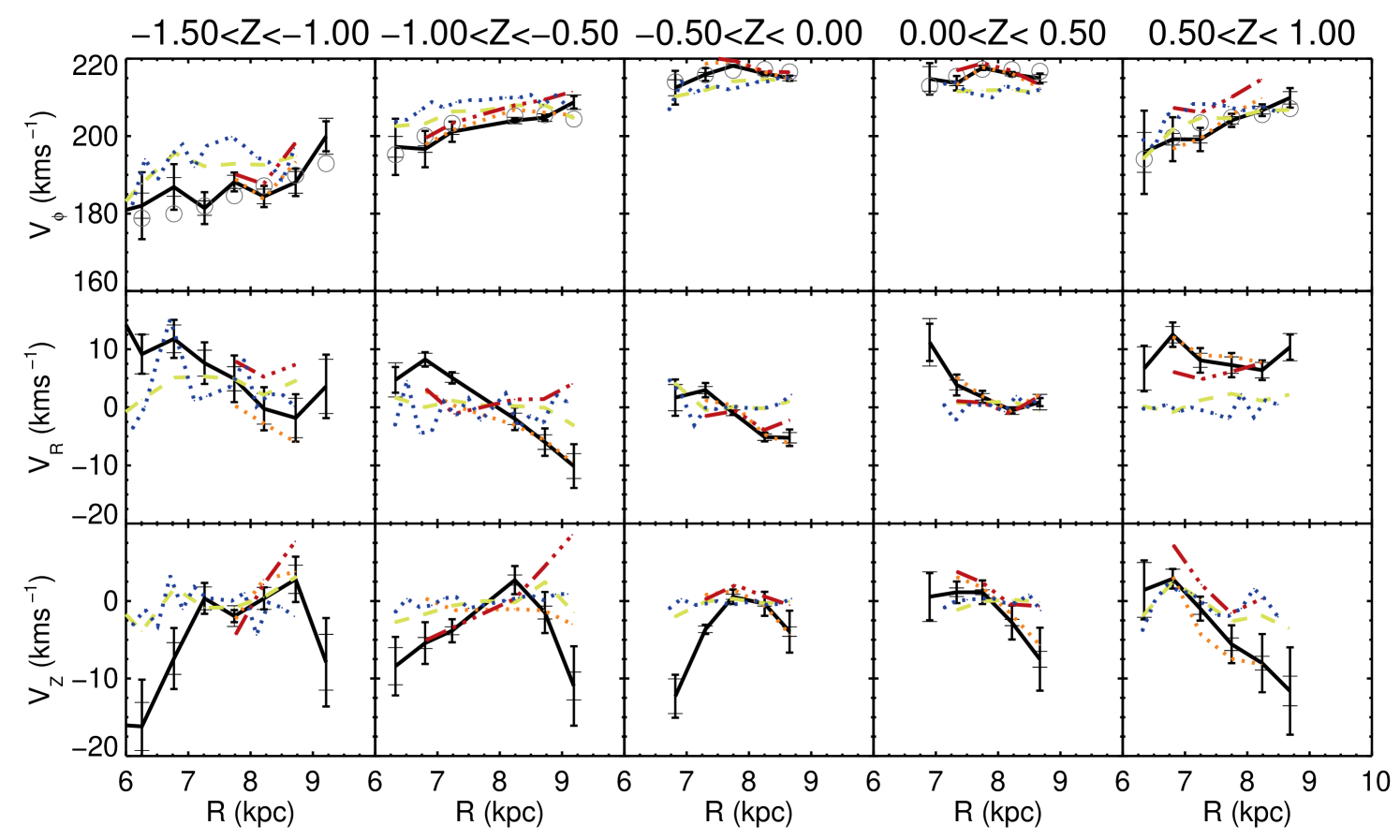
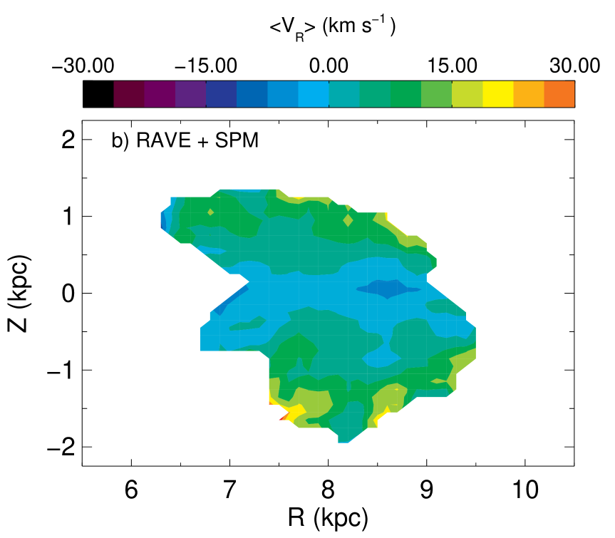
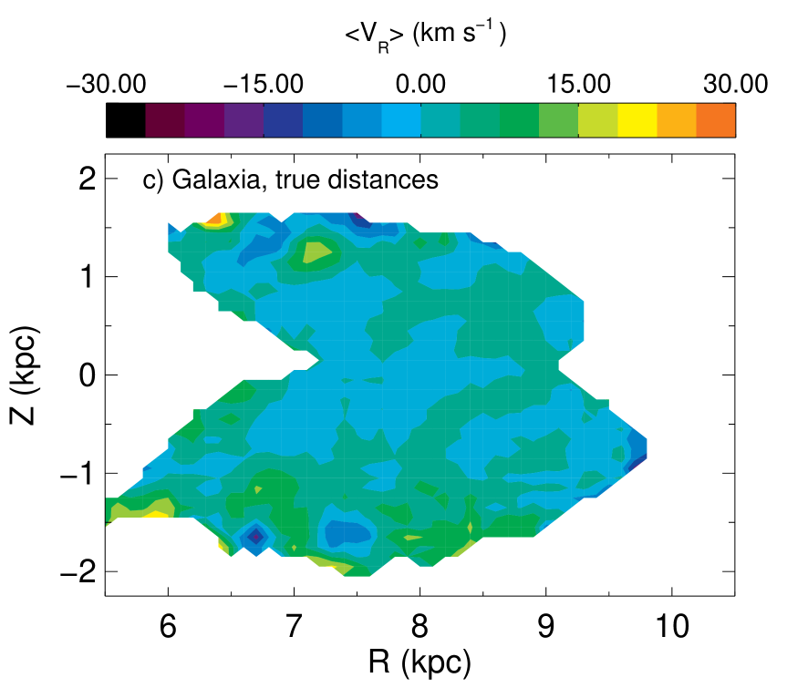
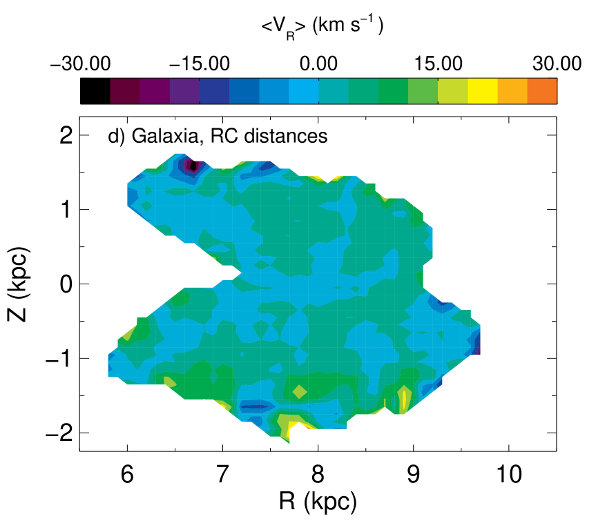
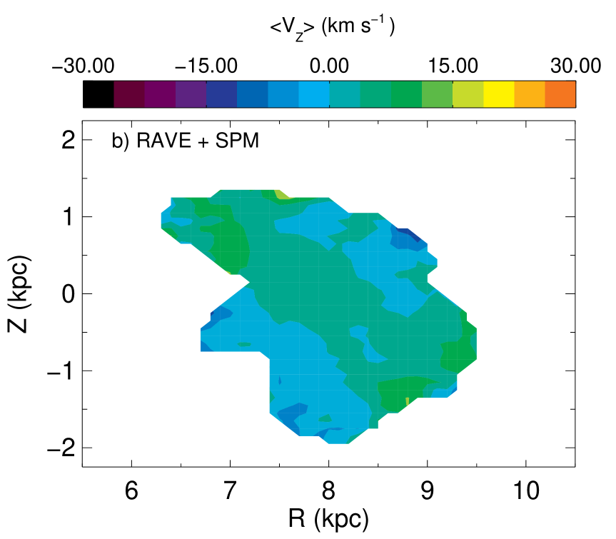
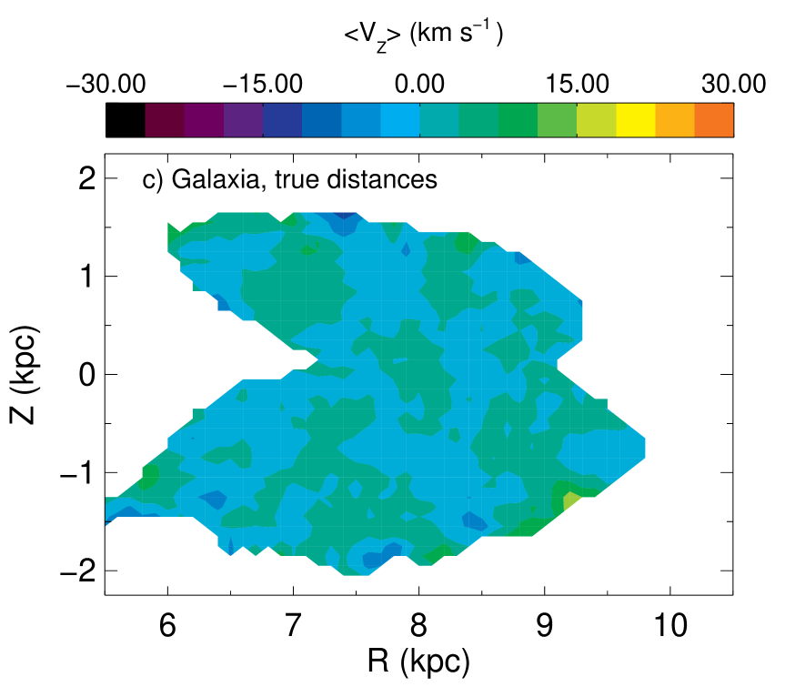
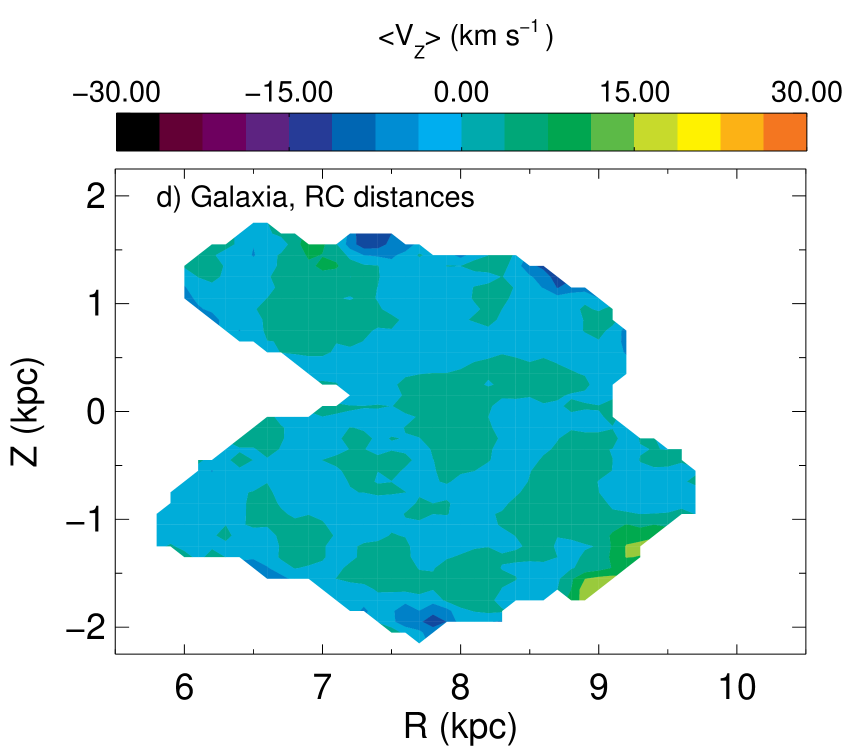
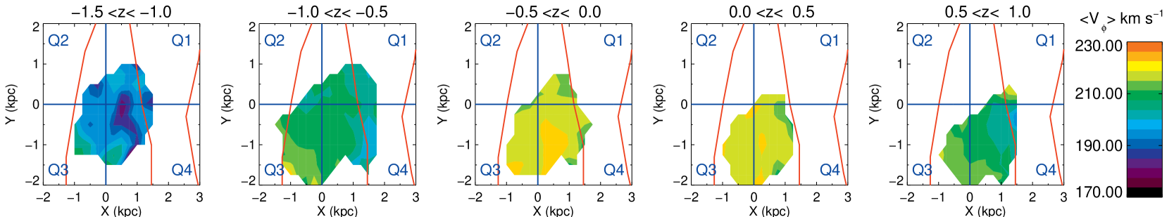
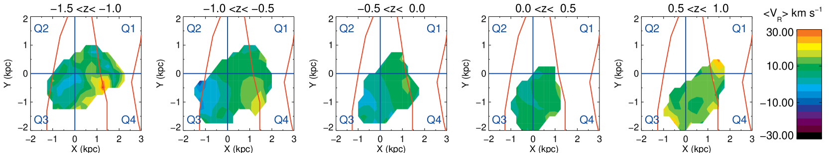
Figure 8 displays the trends in mean (hereafter we drop the bracket notation for averages) as functions of for thick slices in using bins in . Results are shown for three choices of proper motions: those in the RAVE, UCAC3 and SPM4 catalogs. Also shown are the results of the pseudo-data from Galaxia: the blue line is obtained using the true distances to pseudo-stars, while the green line uses distances inferred from RC magnitudes. Figures 10, 12 and 13 display essentially the same results as contour plots in the plane. However, to save space we show results only for the proper motions in the RAVE and SPM4 catalogs and for the Galaxia pseudo-data. The plotted data are box-car averages over wide boxes in with increments in the co-ordinates of the box’s centre. Finally, Figure 14 shows the results obtained with the proper motions in the RAVE catalog in full 3D – are averaged over boxes of size . The centres are moved by in and and spaced by in .
We now discuss the trends in each velocity component.
 |
 |
 |
6.1
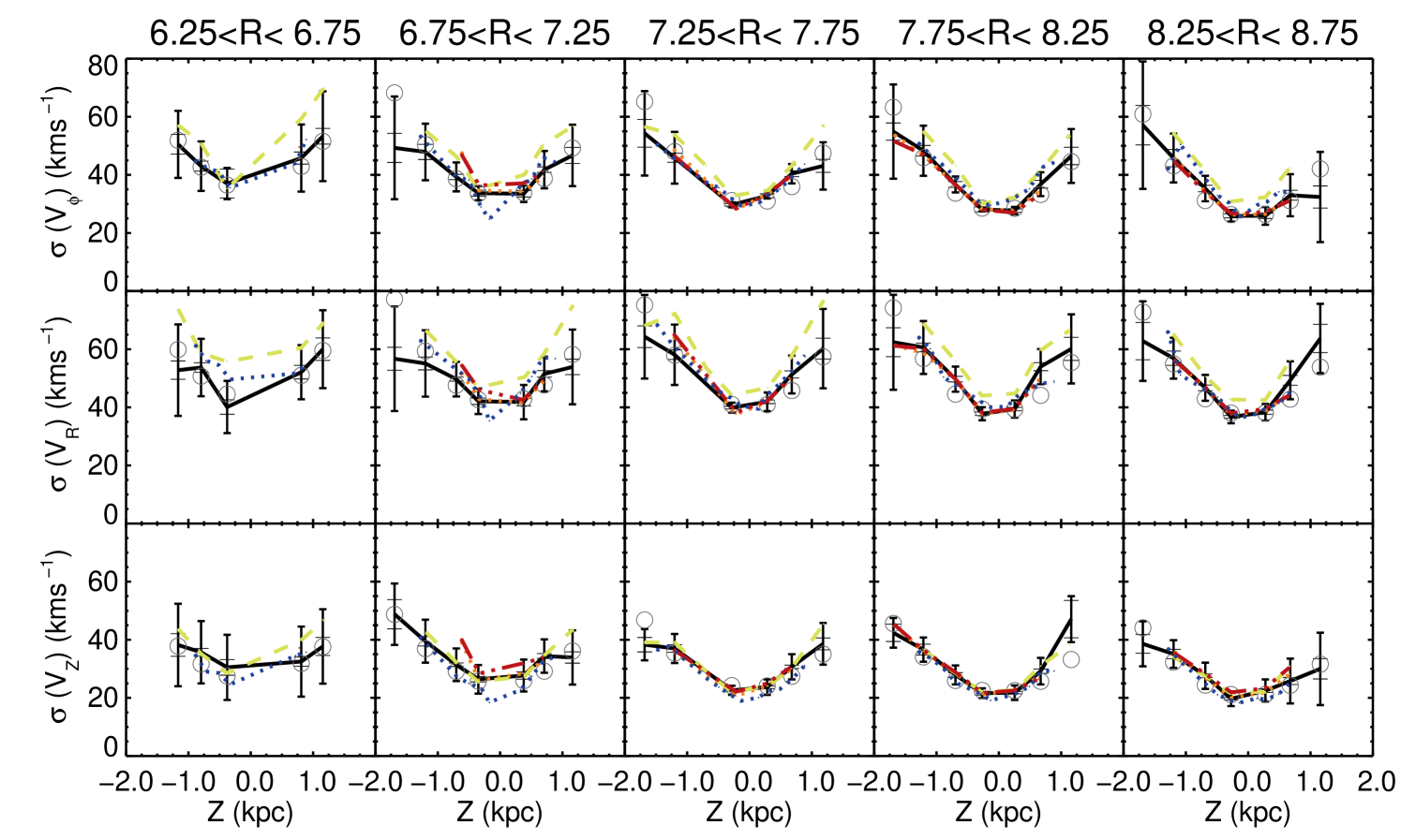
The top two panels of Figure 10 show that, as we might expect, is largest in the plane and decreases fairly symmetrically both above and below the plane. At given values of , also decreases inwards. These trends are independent of the distances used (RC or Zwitter) and of the adopted proper-motion catalog, and they are exactly what the Jeans equations lead us to expect: decreases as the asymmetric drift increases and the asymmetric drift increases with the velocity dispersion (see e.g. Binney & Tremaine, 1998, eq. (4.34)). In Figure 11 the velocity dispersion trends in are shown for the RAVE results and the Galaxia model using the RC-assumption distances. The increase of velocity dispersion with increasing and decreasing is seen in both the data and the model. Consequently, whether we move inwards or away from the plane to regions of increased velocity dispersion, will decrease.
Figure 8 shows that adopting a different proper-motion catalog does slightly change the predicted values of : away from the plane slightly higher values of order are obtained with the SPM4 proper motions than those in the RAVE catalog, while the UCAC3 proper motions give intermediate values (). However, these differences between results from various proper-motion catalogs are smaller than the difference between the observations and the predictions of Galaxia: the latter predicts a markedly flatter profile of with . In other words, the data imply that falls away as we move away from the plane significantly more rapidly than Galaxia predicts. The data give values of greater than Galaxia at , falling below the model at to be lower at .
In Section 4.1.1 we saw that the assumption of a single RC magnitude can lead to an under-estimation of by . This effect is also evident in Figure 8 in that the dotted green lines obtained for the Galaxia model using RC distances lie below the dashed blue lines obtained with the true distances, again by about . Further, in Section 4.1.2 and Figure 5 we saw that for large values of , normalizations B and C give lower values of as large as . The effect was only at the extremities of the data however. Since even the green lines lie above the data for , we conclude that the use of a single RC magnitude or the chosen normalization does not explain the offset between the data and the predictions of Galaxia and the Galaxy’s velocity field must differ materially from that input into Galaxia. Comparison of the top and bottom panels of Figures 10 reveals that, compared to the predictions of Galaxia, the observations show more clearly the expected tendency for to decrease as we move in at fixed .
In their study of the HTDC, Parker et al. 2004 measured the line-of-sight velocities of thick-disk and halo stars, finding that in Quadrant 1 the rotation of this body of stars lagged the LSR by 80-90, while in Quadrant 4 the corresponding lag was only . Far from confirming this effect, the top-left panel of Figure 14 suggests if anything the opposite is true: at and , is lower in the Quadrant 4 than Quadrant 1.
The red curves of Figure 14 show the positions of spiral arms. Close to the plane, at there is some hint that there is an increasing lag in associated with the spiral features. Further from the plane, such an association is less clear, as one might expect.
The dependence of is best described by the power-law:
| (2) |
with Table 4 giving the coefficients for the three different proper motion sources.
The form is not dissimilar to that given for high-metallicity stars in Ivezić et al. 2008 between and () and Bond et al. 2010 between and (). These results are not directly comparable to our fitting formula as we have an extra component that takes radial dependence into account, which may lead to interaction between the fit coefficients. Nevertheless, our range of values for the exponent (1.06-1.38) for the vertical dependence is similar to their results (1.25).
| RAVE catalog | 225 | -51.2 | 2.6 | 1.06 | ||
| SPM4 | 222 | -40.2 | 2.1 | 1.38 | ||
| UCAC3 | 224 | -54.7 | 3.2 | 1.10 |
6.2
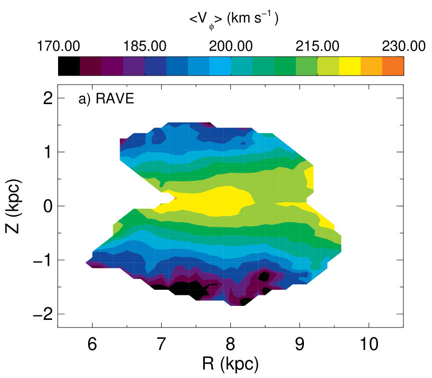
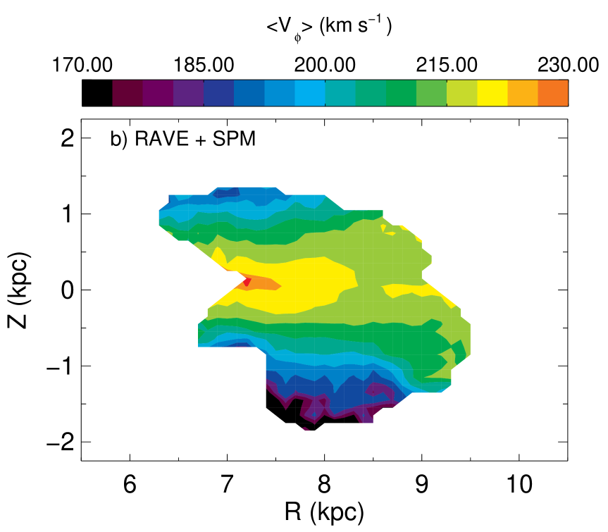
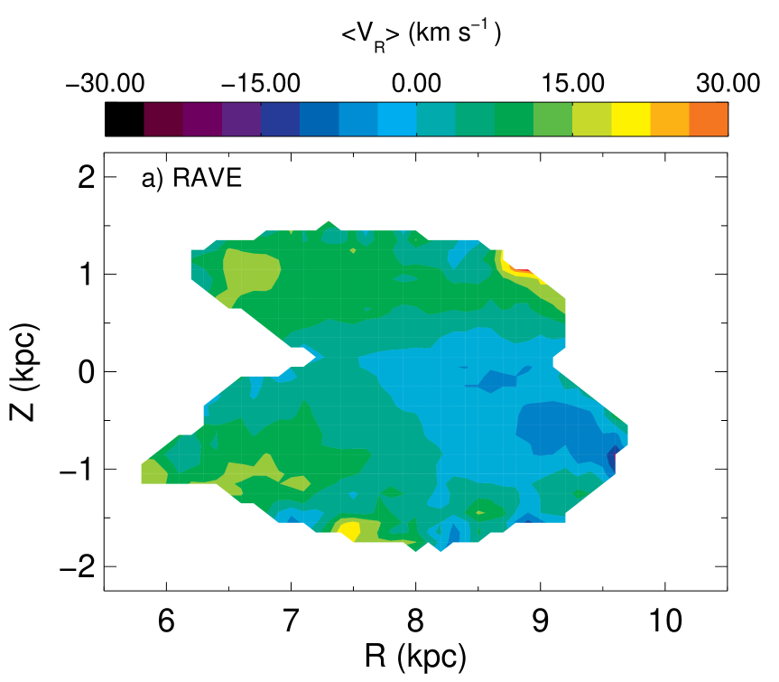
In the top panels of Figure 12, contours of constant are by no means vertical, whether one adopts the proper motions in the RAVE or SPM4 catalogs. In fact, with the SPM4 proper motions the contours are not far from horizontal. Thus the radial gradient reported by S11 is at the very least just one aspect of a complex phenomenon. In fact, if the SPM4 proper motions are correct, the trend in is essentially that the further stars are from the plane, the more they are moving away from the Galactic centre.
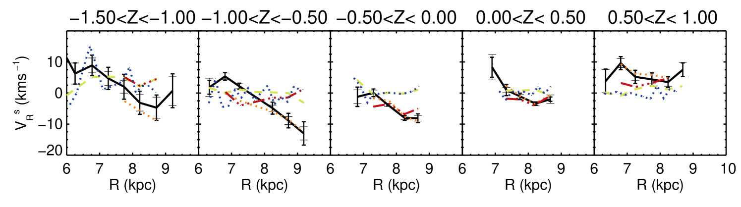
The middle panel of Figure 8 shows this situation in a different way by showing that the red curves for the SPM4 data are horizontal within the errors at all distances from the plane, but they move down from at to zero in the plane and back up to at . In this figure the black curves that join the RAVE data-points tell a different story in that in the panels for they slope firmly downwards to the right. In the two panels for the data points from the RAVE proper motions are consistent with no trend in with with the exception of the innermost point in the panel for , which carries a large errorbar. The present analysis is consistent with the value of reported by S11 in that is roughly the average of the gradient given by the RAVE proper motions at and the vanishing gradient at .
If the dominant gradient in is essentially in the vertical direction and an even function of as the SPM4 proper motions imply, the suspicion arises that it is an artifact generated by the clear, and expected, gradient of the same type that we see in . The gradient could be then seen to be caused by systematics in the proper motions creating a correlation between the measured value of and (see e.g. Schönrich, Binney & Asplund 2012). In Section 7 we re-explore the line-of-sight detection of the , which is a proper-motion-free approach to observing the radial gradient, which however corroborates the existence of a gradient and North-South differences.
Schönrich 2012 found a larger value of compared to that used in this study and S11, and suggest that this larger value would reduce the gradient in . In Figure 9 we plot , the Galactocentric radial velocity with . The qualitative trends are unaffected by the higher value of , with the values only shifted down, bringing the values in the bin closer to those predicted by Galaxia.
In Figure 14 the location of the spiral arms is overlaid for reference on the full plots of trends. There is some indication that structure in is coincident with spiral arms in the region, with Quadrant 3 and Quadrant 4 showing the largest gradient. With a scale height of the thin disk of 300 pc (Gilmore &Reid, 1983), at these large values we would not expect however that spiral resonances would play a role. However, the recent results of S12 which explained the gradient in terms of such resonances suggests that they do exert an influence at large distances from the Galactic plane. The diminishment of the gradient at positive values is also evident in this figure. Further modelling in 3D is required to understand if the North-South differences in the gradient can be explained in terms of resonances due to spiral structure, which one would expect to produce effects symmetric with respect to .
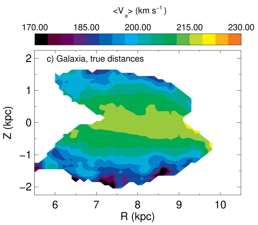
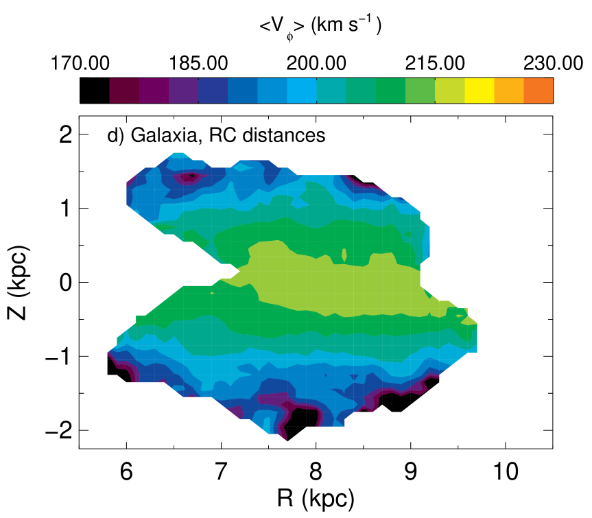
The bottom panels of Figure 12 shows the corresponding Galaxia model for the red clump. Here we see that there is an absence of the observed North-South asymmetry, and further, we confirm that the asymmetry is not produced by using the red clump distance estimate. We have explored the influence of changing the distances using the Zwitter distances. We found that these alternative distance calculations also show the same overall variations for , while exhibiting some differences in various regions. This indicates that while the distances may influence the quantitative results, qualitatively the overall trends remain the same.
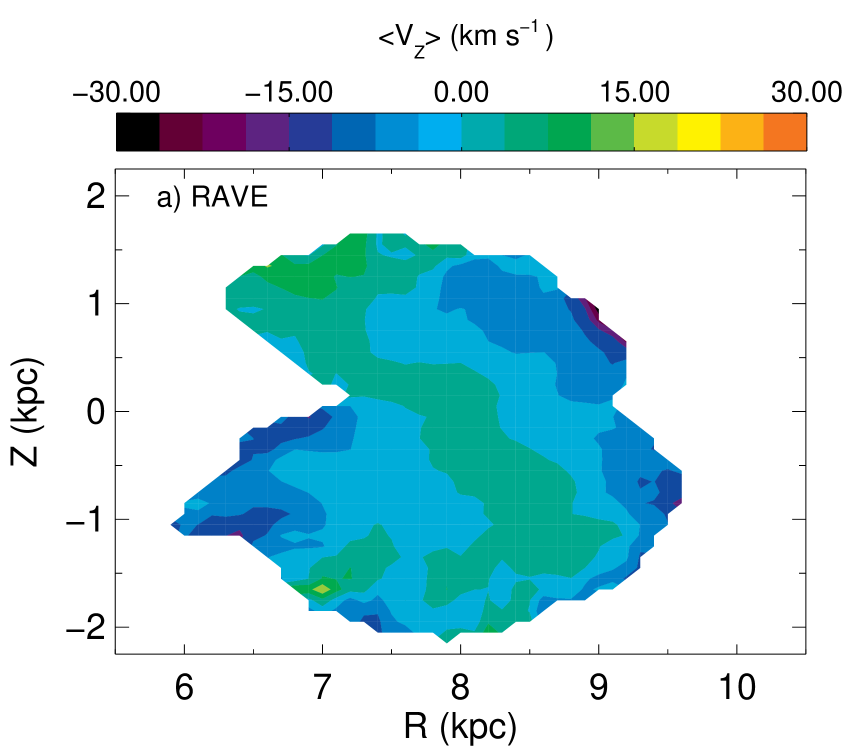
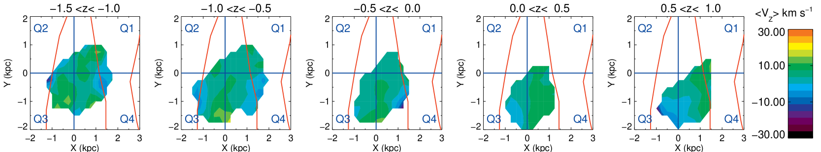
6.3
The top panels of Figure 13 show that both proper-motion catalogs yield a similar dependence of on . We see a ridge of enhanced that slopes across the panel, making an angle of approximately with the axis and cutting that axis at approximately the solar radius. This feature is most pronounced in the bottom-left panel, for proper motions in the RAVE catalog. If we assume the LSR value is zero, and thus the top of the ridge has , we could interpret the stars interior to this point showing an overall rarefaction: stars below the plane move downwards, while those above the plane, move upwards. Exterior to the behaviour is reversed and shows a compression; below the plane stars move upwards, while above the plane stars move downwards. The amplitude of these variations is large; up to as seen from Figure 8.
The results for the SPM4 and UCAC3 proper motions do not exhibit quite so large an amplitude in the variations, but as shown in Figure 13 for SPM4, exhibit a similar overall behaviour, with the line of higher running diagonal across the plane. However, in Figure 8 we see that below the plane, the alternative proper motion results do not show the large dip in at , though this is mostly due to the smaller sampling area in the plane of the alternative proper motion sources. Above the plane, the behaviour of the results from the various proper motion sources is similar, with clear deviation from the Galaxia model’s predictions in the bottom panels of Figure 13. The Galaxia model itself shows a random pattern of high and low of the order of . There is some smoothing spatially of these fluctuations with the use of RC-magnitude derived distances, though the observed pattern is not generated with this distance method. In general, the proper motions dominate the calculated values, and the differences in observed structure reflect this. Nonetheless, it is reassuring that the overall pattern is recovered in Figure 13 with each proper motion catalog source.
Recently, Widrow et al. 2012 found with main-sequence SDSS stars that the vertical number-density and profiles suggest vertical waves in the Galactic disk excited by a recent perturbation. A direct comparison with their results and ours is not possible as their stars are outside the RAVE spatial sampling region. However, our results support this proposition: the rarefaction and compression behaviour seen in the top panels of Figure 13 is indicative of wave-like behaviour. This could then be seen as further “ringing” behaviour of the disk caused by a recent accretion event, as in Minchev et al. 2009; Gomez et al. 2012. Indeed, Gomez et al. 2013 further suggest that such vertical waves may have been excited by the Sagittarius dwarf as it passed through the disk. Their simulations find deviations of up to in in a heavy-Sgr scenario.
Turning now to Figure 14 we find some suggestion that the field shows some alignment with spiral-arms feature, even at significant distances from the plane. Below the plane, the Sagittarius-Carina arm at is aligned with the low velocities seen with the RAVE catalog proper motions for . In this representation, the SPM4 and UCAC3 proper motion results also show a dip in their velocities around this area, though the feature is not as pronounced as for the RAVE catalog proper motions. The Perseus arm is also aligned with an area of lower at . Across all values of , the alignment of the features with the spiral arms is less clear for , which below the plane may be explained by the proximity of the Hercules thick disk cloud.Siebert et al. 2012 showed how spiral density waves could be used to explain the streaming motion. Siebert et al. (in preparation) goes further to investigate how they could also create the structures, coupled to .
These results suggest that there are large-scale vertical movements of stars, with various cohorts at the same moving in opposing directions. In Casetti et al. 2011, it was proposed that while the Galactic warp starts at the solar radius, the small elevations of the warp at these distances ( for (López-Corredoira et al., 2002)) and the large distances of the RAVE stars from the plane would mean that kinematics of stars would be little affected by the warp. In Russiel 2002, the nearby Sagittarius-Carina arm as traced by star-forming complexes is found to lie mostly below the plane by , which suggests that nearby spiral arms can be influenced by some warping. Whether the warp is long-lived or a transient feature would have implications for the associated velocities. The complexity of the vertical velocity distribution suggested by our results would tend to point towards transient features: they suggest a non-equilibrium state. A multi-mode travelling wave caused by a recent accretion event, or structure associated with the disk’s spiral arms, would be the most likely explanations for the observed velocity structure.
6.4 Velocity dispersion trends
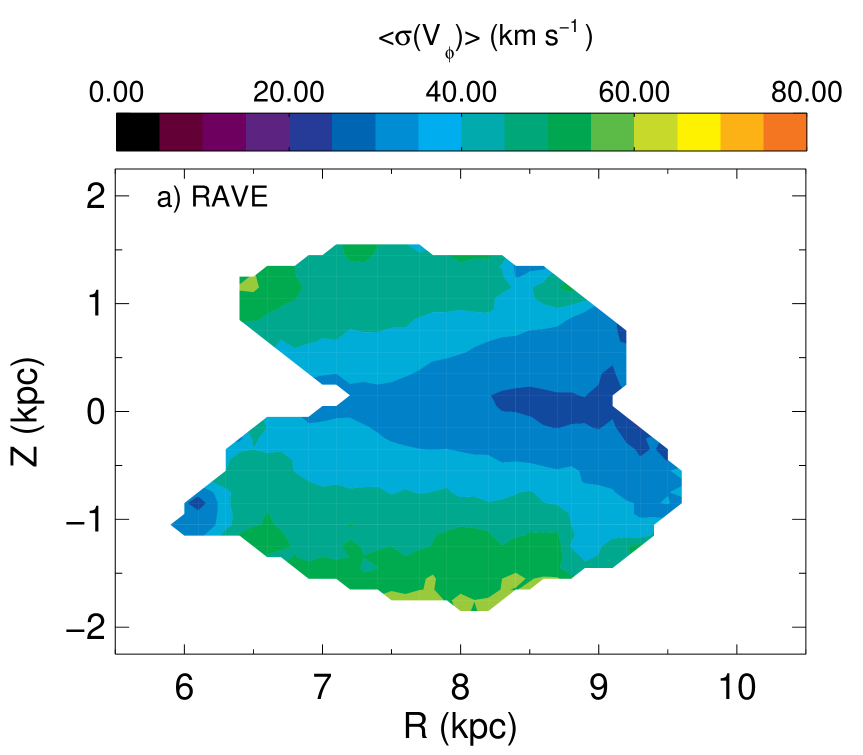
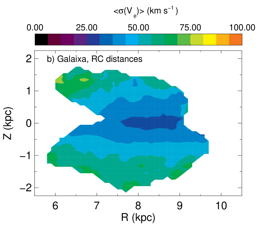
The second moments of the velocity components increase with increasing and decreasing in a smooth fashion as expected, with Figure 11 showing the results for . As for , they can be fit by a simple parametric function.
Figure 15 displays the trends in the dispersion of as a function of for thick slices in using bins in . Also plotted are the results based on UCAC3 and SPM4 proper motions, and the Galaxia model results using the “true” model distances plus RC-calculated distances. Unlike the mean-value trends, the differences between the various proper motion sources is minimal. We see however that the Galaxia model results indicate that the use of RC-calculated distances can lead to an increase in the measured dispersion values, particularly for . Interestingly however, there is a reasonable agreement between the results of Galaxia and that observed with RAVE.
We note that the dispersions were corrected for errors following the same methodology of Casetti et al. 2011. This method adjusts a guess of the true dispersion, , in velocity component until
| (3) |
where , with the MC-derived error in for th star and is the mean over the sample.
The velocity dispersions exhibit linear behaviour in and parabolic behaviour in . Thus, a fit to the dispersion trends was found to be provided by the simple form
| (4) |
with Table 5 giving the coefficients for the three velocity components for the three different proper motion sources. The similar coefficients for each velocity component underlines the similarity of the trends between the three sources.
| RAVE catalog | 67.4 | -5.0 | 12.4 |
|---|---|---|---|
| SPM4 | 75.7 | -6.1 | 15.8 |
| UCAC3 | 71.2 | -5.5 | 15.2 |
| RAVE catalog | 62.6 | -3.0 | 12.5 |
| SPM4 | 60.0 | -2.7 | 15.1 |
| UCAC3 | 63.3 | -3.1 | 13.5 |
| RAVE catalog | 47.0 | -3.1 | 8.2 |
| SPM4 | 49.4 | -3.4 | 9.8 |
| UCAC3 | 43.6 | -2.8 | 10.4 |
7 Velocity gradient: line-of-sight detection
In S11 the gradient in was first investigated using the line-of-sight velocity, , along narrow lines towards the centre and anti-centre. The rationale for this approach was to observe the gradient independent of the proper motions. The complicated 3D structure of the Galactic profile was not considered so we revisit this approach, keeping in mind the 3D trends.
7.1
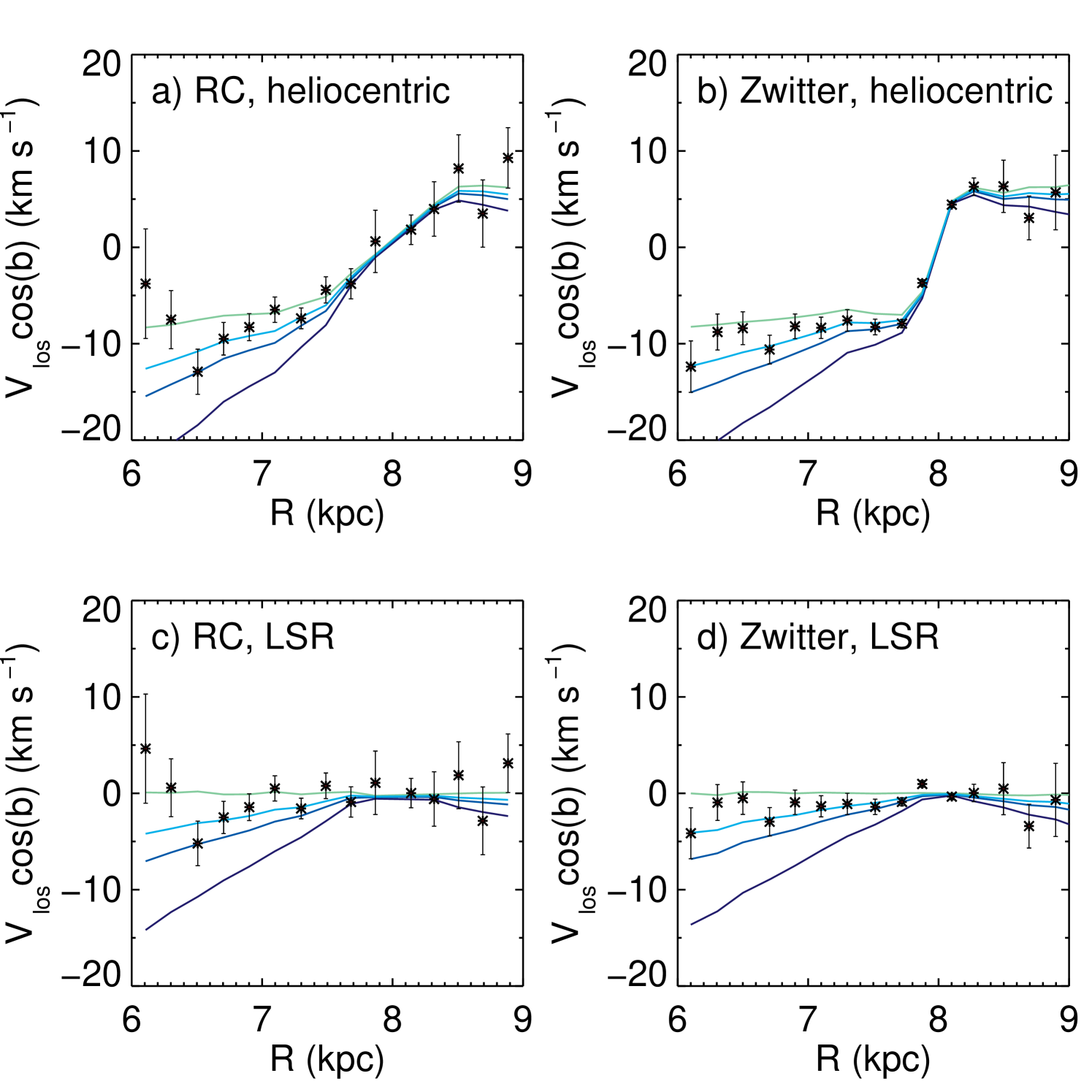
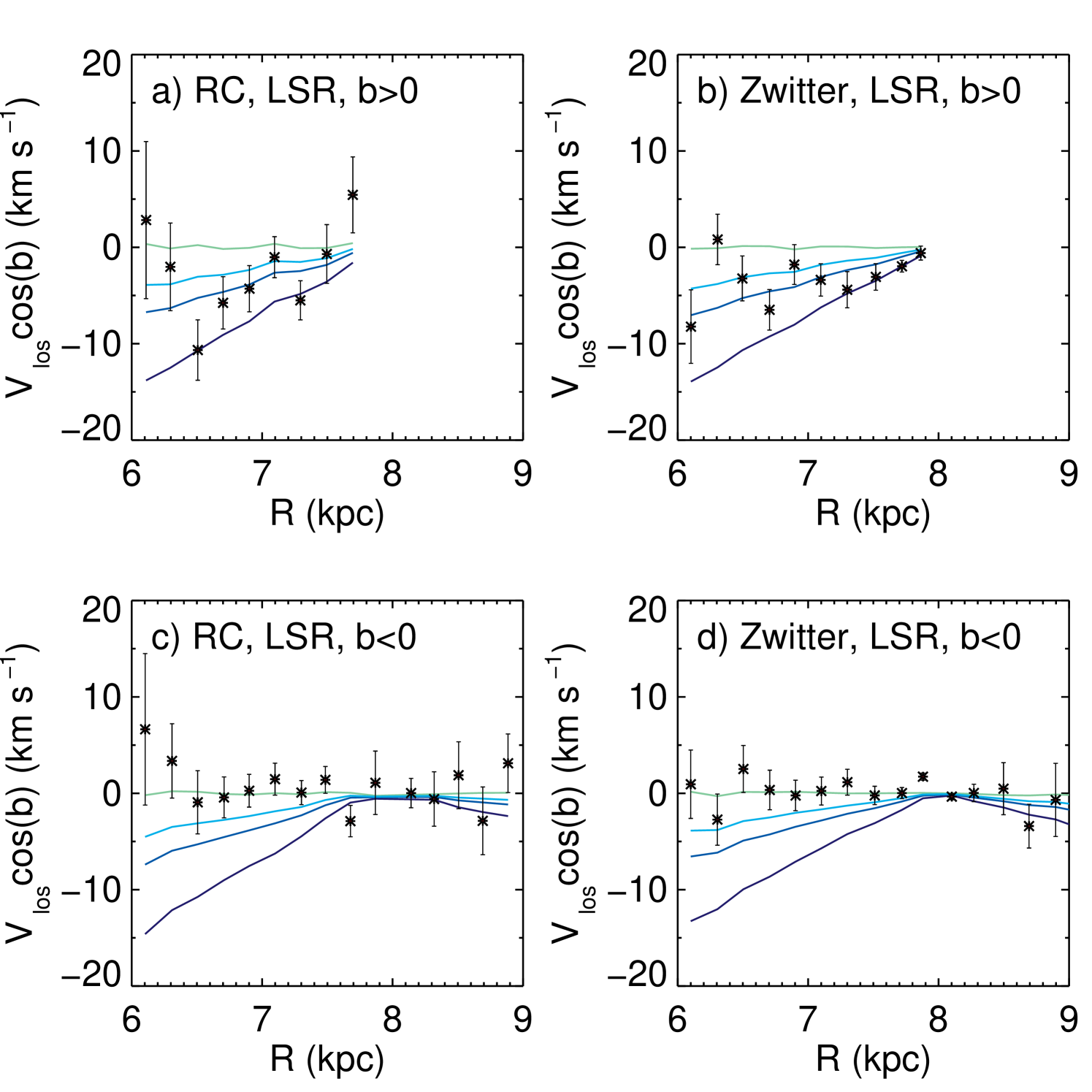
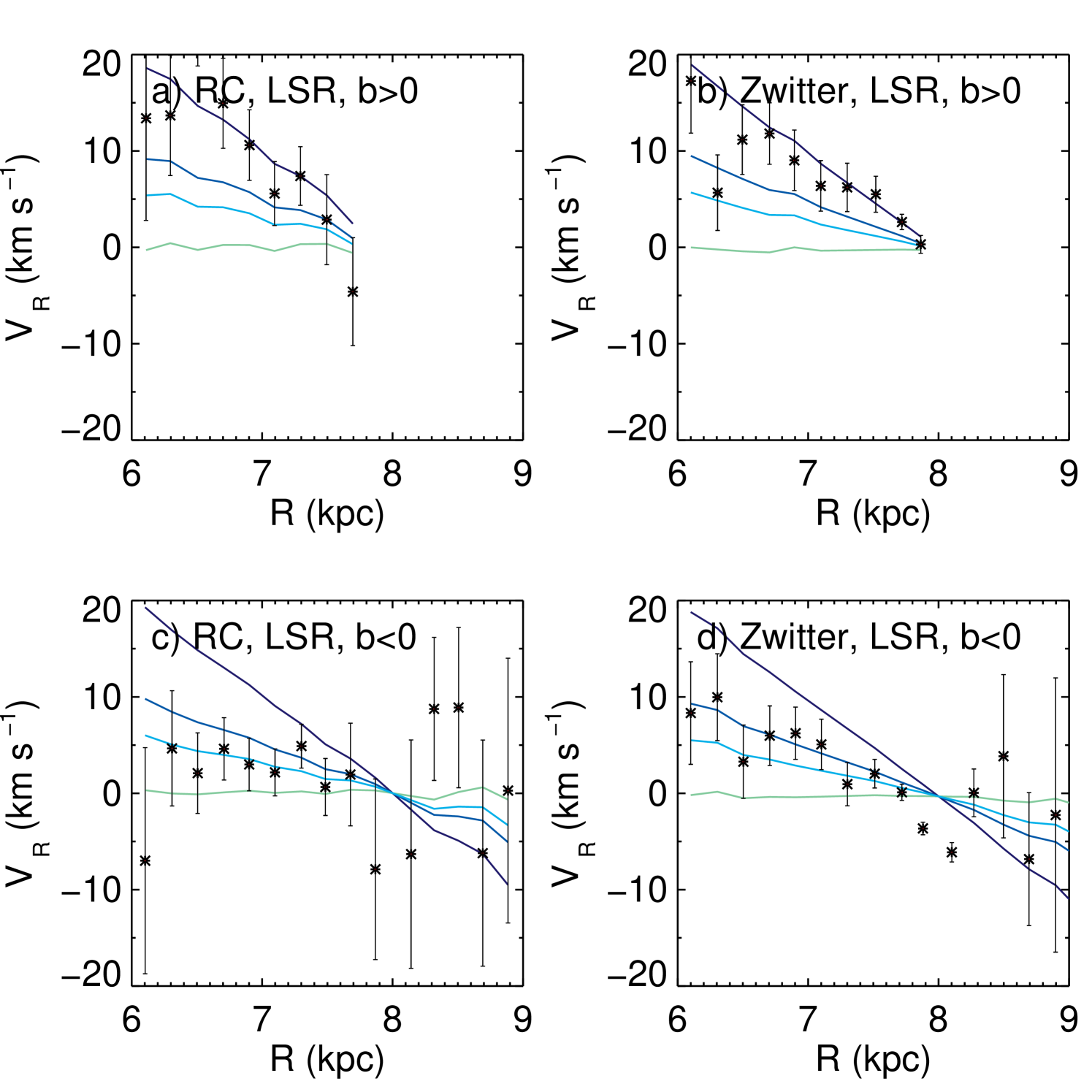
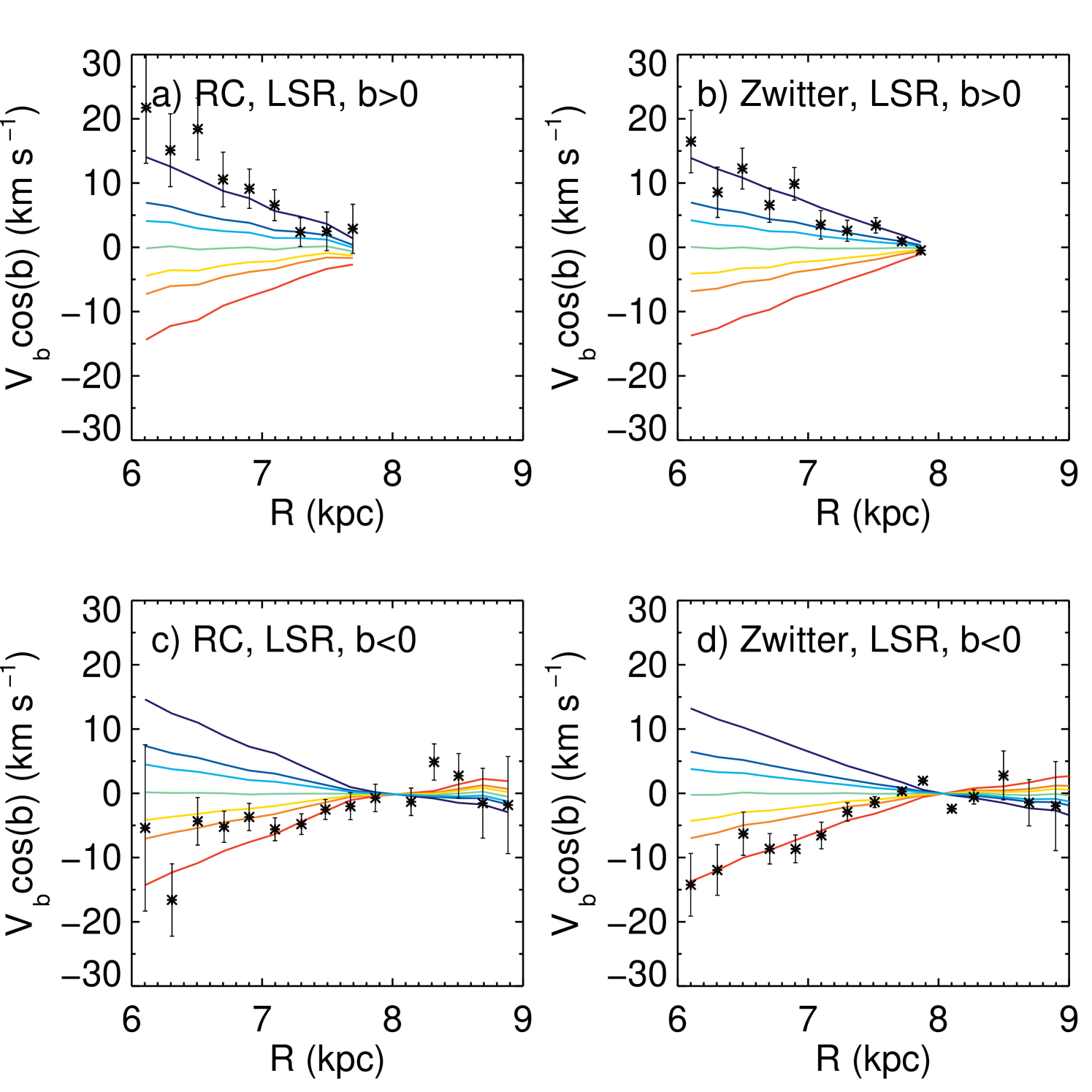
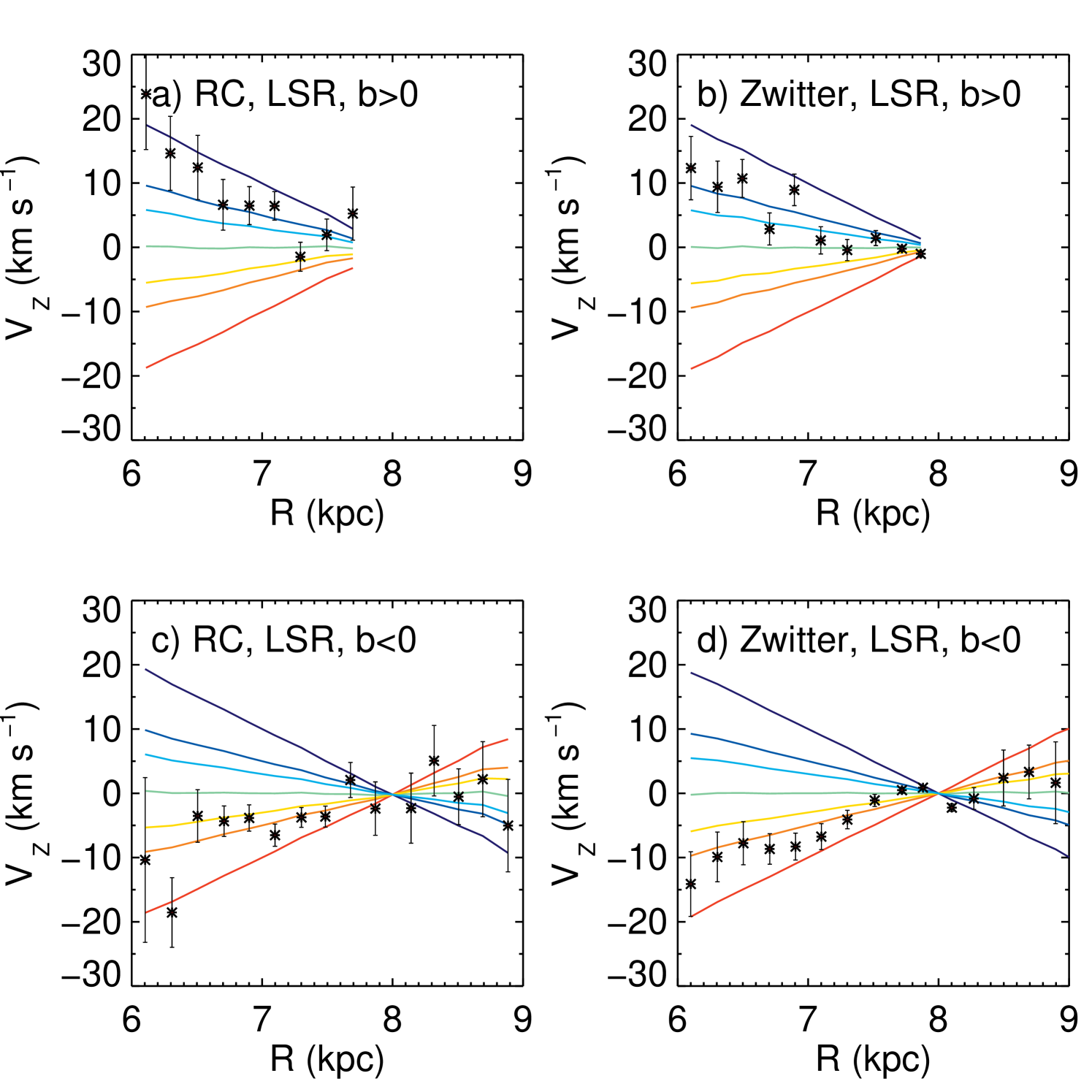
Figure 3 from S11 gives the projection onto the plane of the mean in bins wide as a function of , with the latter a proxy for in their Galactic co-ordinates, with . For and the values of the radial component, is essentially the same as the Cartesian value . As most stars in these narrow cones have , (and so ) is dominated by the term . In the Appendix we list the relevant equations which shows how this follows. S11b compared the mean velocities to those expected for a thin disk in circular rotation and adding a radial gradient of and (plus a thick disk lagging the LSR by ), finding that the results were consistent with a radial gradient of .
From Equations 1 and 7 in the Appendix, we see that if we are to consider the as representative of (and so ), technically it would be better to first subtract the solar motion from the line-of-sight velocity, to obtain . Otherwise the components above and below the plane will be shifted from each other, which can be problematic if the sample shifts from above-the-plane to below-the-plane, potentially producing spurious trends. This was omitted in the analysis of Figure 3 from S11, however, it did not affect the conclusions as the models were similarly shifted.
In Figure 16 we re-examine the trends in for the RC giants and stars with Zwitter distances, where we plot against rather than as this is easier to interpret and there is little difference between the two values. We plot the results with and without the LSR correction, with the curve being flattened in the latter with the removal of the component. We also plot the trends for a thin-disk as in S11, using 100 Monte Carlo realizations. We see here that not correcting for the solar motion does not affect the conclusions. Note that with the updated data sets the streaming motion is slightly less apparent in both the RC and Zwitter results than it was in S11: the model with is a better fit to the data. Also, the differences between the RC and Zwitter trends around the solar radius in Figure 16 is a result of the different geometric sampling of the two.
In Figure 17 we examine the results split into North and South components. In this we open up the criteria a bit to within of the centre and anti-centre direction to reduce the effects of Poisson noise and make the trends clearer. Here we see that that differences can be discerned between the North and South trends, however, they are opposite to that seen in the previous section; the gradient is in the North () is stronger though absent in the South ()) for . Plotting the corresponding results for in Figure 18, we find that the including the proper motion results shifts the overall values so that the northern trends are more in line with and the southern . Despite the disparity with the actual numbers, the cause of which is discussed below, both and the nonetheless exhibit differences between the north and south trends, opposite to those found in Section 6.2.
To understand the reversal of the trends note first that the selected sample cuts across a range of as we change so these plots combine the and trends seen previously. Second, the necessary restriction on means that we are sampling a very narrow beam and thus do not see the global patterns, but only those along that beam. In Figure 14 Quadrants 3 and 4 show the largest gradient, which we miss with the beams. Hence, these plots emphasize the 3D nature of the values in the solar neighbourhood: what you measure very much depends on where you look, be it north or south, and at different and values.
7.2
From Equation 6 in the Appendix we can see that can be used as a proxy for if . This condition is for the most part met in the low latitudes sampled along the and cones used above. So in Figure 19 we examine the trends above and below the plane for in these directions, with Figure 20 giving the corresponding trends in the total . Note that we use RC and Zwitter distances here to provide the abscissa, supplementing the proper motion data. We also plot both positive and negative trends in for a thin disk model as above, with values from .
Both Figures 19 and 20 show that the trends above and below the plane are markedly different, with the decreasing with R above the plane at a rate of according to the plot and , to the plot. Below the plane, there is a positive trend of in both plots. This positive trend in appears to stop just beyond the solar circle at . In contrast to above, this behaviour is consistent with what was found in Section 6.3.
Note that the differences between the observed magnitude of the trends in and , plus and can be explained by the fact that both and contain components of and . For small , and . The cross-terms mean that there is some ‘leakage’ of the trends into and trends into , which work to either diminish or enhance the observed trend in the single component. Nonetheless, the fact that there are differences between the north and south for the single components at all is further evidence of the 3D variations of the velocity values.
The and trends, as seen via the line-of-sight velocities and proper motions respectively, are unaffected by potential systematics in the distances: a change of the distance scale would not affect the fact that a trend is seen at all. This is particularly so for the differences observed between the northern and southern samples. Furthermore, both the SPM and UCAC3 proper motions give similar results as in Figures 19, with a stark negative trend above the plane and a positive trend below for the region . Thus, neither the distances nor the proper motions introduce large systematics into this method of detection.
8 Conclusion
Using RAVE red clump giants we have examined in detail the first moments of the velocity components in a large volume around the Sun. We find differences between the North and South in the streaming motion reported in Siebert et al. 2011 in Galactocentric radial velocity, . Above the plane, there is a large outward flow ( for ) with a shallow or non-existent gradient. Below the plane, there are lower values of outside the solar circle, down to at . This is associated with a much steeper gradient in , particularly in Quadrants 3 and 4, the largest gradient being for .
The behaviour of shows a surprising complexity suggestive of a wave of compression and rarefaction: there is a ridge of higher passing at an angle of to the plane, intersecting the plane at roughly the solar radius. Assuming the LSR to be zero, stars interior to the solar circle and above the plane are moving upwards, while those below the plane, downwards. Exterior to the solar circle, stars both above and below are moving on average towards the plane. Values of up to are observed. We confirm these differences by examining the transverse velocities along narrow cones towards- and away-from the Galactic centre.
Physically, the velocity field implies alternate rarefaction and compression, as in a sound wave. Thus our three-dimensional velocity field confirms the recent one-dimensional results of Widrow et al. 2012 in which North-South differences in the velocities of SDSS stars suggested vertical waves in the Galactic disk. Two likely causes of these waves are either a recently accreted satellite or the disk’s spiral arms. Further modelling will hopefully help decide between these two scenarios.
is much more regular than the other two components, showing the most qualitative agreement with the mock sample created with the Galaxia model for the Galaxy and the expected increase of with increasing and decreasing . The model gives a much flatter profile of with however than the data; at we measure values larger than Galaxia, falling to lower at . There is some hint of an increased lag in near the plane associated with spiral arm features. We present a simple parametric fit to the dependence on and .
We also trace the second moments of the velocities as a function of and , providing a simple parametric fit to these trends as well.
The red clump is increasingly being used as a standard candle for field stars, given its ease of identification and the relative insensitivity of the magnitude to age and metallicity. We modelled our selection of RC stars using Galaxia, showing a surprisingly high level of contamination by first-ascent giants despite a tight selection in the - plane. However, given that the majority of these giants have a similar magnitude to the red clump itself, the effect on the distances does not render them unusable. It means though that there is further complexity in the metallicity-age mixture of selected red clump stars: the population is by no means homogenous in age and abundance.
The assumption of a single magnitude for the RC and the proper motions are the largest sources of systematic error in our analysis. Indeed, a deeper study into proper motion differences is required to establish which of the catalogs is most trustworthy. Nevertheless, we have established that North-South differences do exist in and despite these problems. For a line-of-sight detection, which excludes the proper motions, shows gradients above and below the plane despite the pencil beams in this analysis pointing away from the area of the largest gradient in Quadrants 3 and 4. These results particularly illustrate the 3D nature of the velocity field. For , results using the three proper motion sources give the same rarefaction-compression behaviour, albeit with some variation in the details.
The 3D structure in and presents challenges to future modelling of the Galactic disk under the influence of the bar, spiral features and any other perturbations (be they temporally localised or not). It is not intrinsically clear indeed if the structure in the two are coupled or arise from different physical mechanisms.
Acknowledgments
Funding for RAVE has been provided by: the Australian Astronomical Observatory; the Leibniz-Institut fuer Astrophysik Potsdam (AIP); the Australian National University; the Australian Research Council; the French National Research Agency; the German Research Foundation (SPP 1177 and SFB 881); the European Research Council (ERC-StG 240271 Galactica); the Istituto Nazionale di Astrofisica at Padova; The Johns Hopkins University; the National Science Foundation of the USA (AST-0908326); the W. M. Keck foundation; the Macquarie University; the Netherlands Research School for Astronomy; the Natural Sciences and Engineering Research Council of Canada; the Slovenian Research Agency; the Swiss National Science Foundation; the Science & Technology Facilities Council of the UK; Opticon; Strasbourg Observatory; and the Universities of Groningen, Heidelberg and Sydney. The RAVE web site is at http://www.rave-survey.org.
We are grateful to the referee for a number of helpful suggestions which improved the paper.
References
- Abadi et al. (2003) Abadi, M. G., Navarro, J. F., Steinmetz, M., and Eke, V. R. 2003, ApJ, 597, 21.
- Alonso, Arribas & Martinez-Roger (1996) Alonso, A., Arribas, S., and Martinez-Roger, C. 1996, A&A, 313, 873
- Alves (2000) Alves, D. R. 2000, ApJ, 539, 732
- Antoja et al. (2009) Antoja, T., Valenzuela, O., Pichardo, B., Moreno, E., Figueras, F. and Fernández, D. 2009, ApJ, 700, 78
- Antoja et al. (2012) Antoja, T., Helmi, A., Famaey, B. et al. 2012, MNRAS, 426, 1
- Beers et al. (2000) Beers, T. C., Chiba, M., Yoshii, Y., Platais, I., Hanson, R. B., Fuchs, B., and Rossi, S. 2000, AJ, 119, 2866
- Bessell & Brett (1989) Bessell, M. S. and Brett, J. M. 1989, in Infrared Extinction and Standardization, ed. E. F. Milone, volume 341 of Lecture Notes in Physics, Berlin Springer Verlag, 61
- Binney & Tremaine (1998) Binney, J. and Tremain, S. 1998, Galactic Dynamics, Princeton Univ. Press, Princeton NJ
- Boeche et al. (2011) Boeche, C., Siebert, A., Wiliams M. et al. 2011, AJ, 142, 193
- Bond et al. (2010) Bond, N. A., Ivezić, Ž, Sesar, B. et al. 2010, ApJ, 716, 1
- Burnett et al. (2011) Burnett, B., Binney, J., Sharma, S.. et al. 2011, A&A, 532, 113
- Cannon et al. (1970) Cannon,R. D. 1970, MNRAS, 150, 111
- Carpenter (2003) Carpenter, J. 2003, Based on Carpenter 2001, ApJ 121, 2851
- Casetti et al. (2011) Casetti-Dinescu, D. I., Girard, T. M., Korchagin, V. I. and van Altena, W. F., ApJ, 728, 7
- Chakrabarty (2007) Chakrabarty, D. 2007, A&A, 467, 145
- De Silva et al. (2007) De Silva, G. M., Freeman, K. C., Bland-Hawthorn, J., Asplund, M., and Bessell, M. S. 2007, AJ, 133, 694
- De Simone, Wu & Tremaine (2004) De Simone, R., Wu, X. and Tremaine, 2004, MNRAS, 350, 627
- Dehnen (1998) Dehnen, W. 1998, AJ, 115, 2384
- Dehnen (1999) Dehnen, W. 1999, ApJL, 524, 35
- Englmaier, Pohl and Bissantz (2008) Englmaier,P., Pohl, M., and Bissantz, N., 2008, in Corsini, E. N., Debattista,V. P., eds. Memorie della Società Astronomica Italiana, Padova, Italy, p.199 (arXiv:0812.3491)
- Famaey et al. (2005) Famaey, B., Jorissen, A., Luri, X., Mayor, M., Udry, S., Dejonghe, H., and Turon, C. 2005, A&A, 430, 165
- Famaey et al. (2007) Famaey, B., Pont, F., Luri, X., Udry, S., Mayor, M. and Jorissen, A. 2007, A&A, 461, 957
- Girard et al. (2011) Girard, T. M., van Altena, W. F., Zacharias, N. et al. 2011, AJ, 142, 15
- Gilmore &Reid (1983) Gilmore, G. and Reid, N. 1983, MNRAS, 202,1025
- Groenewegen (2008) Groenewegen, M. A. T. 2008, A&A, 488, 935
- Grocholski & Sarajedini (2002) Grocholski, A. J. and Sarajedini, A. 2002, AJ, 123, 1603
- Gomez et al. (2012) Gómez, F. A., Minchev, I., Villalobos, Á., O’Shea, B. W. and Williams, M. E. K. 2012, MNRAS, 419, 2163
- Gómez et al. (2012) Gómez, F. A., Minchev, I., O’Shea, B. W., et al. 2012, MNRAS, 423, 3727
- Gomez et al. (2013) Gómez, F. A., Minchev, I., O’Shea, B. W., Beers, T. C., Bullock, J. S. and Purcell, C. W. 2012, MNRAS, 429, 159
- Guedes et al. (2011) Guedes, J. and Callegari, S. and Madau, P. and Mayer, L. 2011, ApJ, 742, 76
- Helmi et al. (1999) Helmi, A., White, S. D. M., de Zeeuw, P. T., and Zhao, H. 1999, Nature, 402, 53
- Humphreys et al. (2011) Humphreys, R. M., Beers, T. C., Cabanela, J. E., Grammer, S., Davidson, K., Lee, Y. S. and Larsen, J. A., 2011, AJ, 141, 131
- Ibata, Gilmore & Irwin (1994) Ibata, R. A., Gilmore, G., and Irwin, M. J. 1994, Nature, 370, 194
- Jurić et al. (2008) Jurić, M., Ivezić, Z., Brookes, A., et al. 2008, ApJ, 673, 864
- Ivezić et al. (2008) Bond, N. A., Ivezić, Ž., Sesar, B. et al. 2008, ApJ, 684, 287
- Kazantzidis et al. (2008) Kazantzidis, S., Bullock, J. S., Zentner, A. R., Kravtsov, A. V. and Moustakas, L. A. 2008, ApJ, 688, 254
- Kordopatis et al. (2011) Kordopatis, G., Recio-Blanco, A., de Laverny, P., et al. 2011, A&A, 535, A106
- Larsen & Humphreys (1996) Larsen, J. A. and Humphreys, R. M. 1996, ApJ, 468, L99
- Larsen, Humphreys & Cabenela (2008) Larsen, J. A., Humphreys, R. M. and Cabanela, J.E. 1996, ApJ, 468, L99
- Larsen, Cabenela & Humphreys (2011) Larsen, J. A. , Cabanela, J. E. and Humphreys, R. M. 2011, ApJ, 141, 130
- López-Corredoira et al. (2002) López-Corredoira, M., Cabrera-Lavers, A., Garzón, F. and Hammersley, P. L. 2002, A&A, 394, 883
- Majewski et al. (2003) Majewski, S. R., Skrutskie, M. F., Weinberg, M. D. and Ostheimer, J. C. 2003, AJ, 599, 182
- Matijevič et al. (2010) Matijevič, G., Zwitter, T., Munari, U. et al. 2010, AJ, 140, 184
- Matijevič et al. (2011) Matijevič, G., Zwitter, T., Bienaymé, O. et al. 2011, AJ, 141, 200
- Matijevič et al. (2012) Matijevič, G., Zwitter, T., Bienaymé, O. et al. 2012, ApJS, 200, 14
- Minchev et al. (2009) Minchev, I., Quillen, A. C., Williams, M., Freeman, K. C., Nordhaus, J., Siebert, A. and Bienaymé, O., 2009, MNRAS, 396, 56
- Minchev et al. (2010) Minchev, I., Boily, C., Siebert, A., & Bienayme, O. 2010, MNRAS, 407, 2122
- Momany et al. (2006) Momany, Y., Zaggia, S., Gilmore, G., Piotto, G., Carraro, G., Bedin, L. R. and de Angeli, F.. 2006, A&A, 451, 515
- Newberg et al. (2002) Newberg, H. J. and Yanny, B. and Rockosi, C. et al. 2002, ApJ, 569, 245
- Pasetto et al. (2012a) Pasetto, S., Grebel, E. K. and Zwitter, T. et al. 2012, A&A, 547, 70
- Pasetto et al. (2012b) Pasetto, S., Grebel, E. K. and Zwitter, T. et al. 2012, A&A, 547, 71
- Parker et al. (2003) Parker, J. E., Humphreys, R. M. and Larsen, J. A. 2003, AJ, 126, 1346
- Parker et al. (2004) Parker, J. E., Humphreys, R. M. and Beers, T. C. 2004, AJ, 127, 1567
- Penarrubia et al. (2005) Peñarrubia, J., Martínez-Delgado, D., Rix, H. W., et al. 2005, ApJ, 626, 128
- Pietrzyński, Gieren & Udalski (2003) Pietrzyński, G., Gieren, W., and Udalski, A. 2003, AJ, 125, 2494
- Pompéia et al. (2011) Pompéia, L., Masseron, T., Famaey, B., et al. 2011, MNRAS, 415, 1138
- Quillen & Minchev (2005) Quillen, A. C. and Minchev, I. 2005, AJ, 130, 576
- Quillen et al. (2011) Quillen, A. C., Dougherty, J., Bagley, M. B., Minchev, I., & Comparetta, J. 2011, MNRAS, 417, 762
- Raboud et al. (1998) Raboud, D., Grenon, M., Martinet, L., Fux, R., and Udry, S. 1998, A&A, 335, 61
- White & Rees (1978) White, S. D. M. and Rees, M. J. 1978, MNRAS, 183, 341
- Roeser et al. (2008) Röser, S., Schilbach, E. , Schwan, H., Kharchenko, N. V., Piskunov, A. E. and Scholz, R.-D. 2008, A&A, 488, 401
- Roeser et al. (2010) Roeser, S., Demleitner, M. and Schilbach, E. 2010, AJ, 139, 2440
- Russiel (2002) Russiel, D. 2002, A&A, 397, 133
- Salaris & Girardi (2002) Salaris, M. and Girardi, L. 2002, MNRAS, 337, 332
- Schlegel et al. (1998) Schlegel, D. J., Finkbeiner, D. P., and Davis, M. 1998, ApJ, 500, 525
- Schönrich, Binney & Dehnen (2010) Schönrich, R., Binney, J., and Dehnen, W. 2010, MNRAS, 403, 1829
- Schönrich, Binney & Asplund (2012) Schönrich, R., Binney, J., and Asplund, M. 2012, MNRAS, 420, 1281
- Schönrich (2012) Schönrich, R. 2012, MNRAS, 427, 274
- Sharma et al. (2011) Sharma, S., Bland-Hawthorn, J., Johnston, K. & Binney, J.J. 2011, ApJ, 730, 3
- Siebert et al. (2011) Siebert, A. and Famaey, B. and Minchev, I., et al. 2011, MNRAS, 412, 2026
- Siebert et al. (2011b) Siebert, A., Williams, M., Siviero, A., et al. 2011, AJ, 141, 187
- Siebert et al. (2012) Siebert, A., Famaey, B., Binney, J., et al. 2012, MNRAS, 425, 2335
- Skuljan, Cottrell & Hearnshaw (1997) Skuljan, J., Cottrell, P. L. and Hearnshaw, J. B., 1997, ESASP, 402, 525
- Steinmetz et al. (2006) Steinmetz, M., Zwitter, T., Siebert, A., et al. 2006, AJ, 132, 1645
- Tonry & Davis (1979) Tonry, J. and Davis, M. 1979, AJ, 84, 1511
- van Helshoecht & Groenewegen (2007) van Helshoecht, V. and Groenewegen, M. A. T. 2007, A&A, 463, 559
- van Leeuwen (2007) van Leeuwen, F. 2007, Hipparcos, the new reduction of the Raw Data, ASSL 350, Springer
- Vallenari et al. (2006) Vallenari, A., Pasetto, S., Bertelli, G., Chiosi, C., Spagna, A., and Lattanzi, M. 2006, A&A, 451, 125
- Williams et al. (2011) Williams, M.E.K., Steinmetz, M., Sharma, S. et al. 2011, ApJ, 728, 102
- Widrow et al. (2012) Widrow, L.M., Gardner, S., Yanny, B., Dodelson, S. and Chen, H. 2012, ApJL, 750, 41
- Yanny et al. (2003) Yanny, B. and Newberg, H. J. and Grebel, E. K. et al. 2003, ApJ, 588, 824
- Yasuda, Fukugita & Schneider (2007) Yasuda, N., Fukugita, M., and Schneider, D. P. 2007, AJ, 134, 698
- Zacharias et al. (2004) Zacharias, N., Urban, S. E., Zacharias, M. I., Wycoff, G. L., Hall, D. M., Monet, D. G. and Rafferty, T. J. 2004, AJ, 127, 3043
- Zacharias et al. (2010) Zacharias, N., Finch, C., Girard, T et al. 2004, AJ, 139, 2184
- Zwitter et al. (2008) Zwitter, T., Siebert, A., Munari, U., et al. 2008, AJ, 136, 421
- Zwitter et al. (2010) Zwitter, T., Matijevič, G. and Breddels et al. 2010, A&A, 522, 54
Appendix
The peculiar motion of the Sun is given in the Cartesian values . We define the line-of-sight velocity and proper motion vectors in co-ordinates corrected for reflex of the solar motion:
| (5) | |||
| (6) | |||
| (7) |
The reason we do the correction this way round (rather than simply in ) is because we wish to see how the line-of-sight velocities and proper motions are constituted. For example, the Sun is moving up towards the Galactic pole. To correct for this in the line-of-sight velocity when looking above and below the plane this contribution from is subtracted and added respectively. Hence, the solar motion must be corrected for before examining trends in , especially if averaging over positive and negative .
The components are given by
| (8) | |||
| (9) | |||
| (10) |
where is positive towards the Galactic centre. For small this reduces to
| (11) | |||
| (12) | |||
| (13) |
Similar results are obtained near , obviously with some sign changes. To convert to cylindrical co-ordinates we firstly define the Cartesian values corrected for the circular velocity at the solar radius;
| (14) | |||
| (15) | |||
| (16) |
where we use the nominal value in the majority of this paper. The cylindrical components are then
| (17) | |||
| (18) | |||
| (19) |
with . For the small (or ) discussed in Section 7 where , and for the solar neighbourhood where , these reduce to and and so these values are interchangeable in this regime.