The X-ray outburst of PG 1553+113: A precession effect of two jets in the supermassive black hole binary system
Abstract
Blazar PG 1553+113 is thought to be a host of supermassive black hole binary (SMBHB) system. A 2.2-year quasi-periodicity in the -ray light curve was detected, possibly result of jet precession. Motivated by the previous studies based on the -ray data, we analyzed the X-ray light curve and spectra observed during 2012–2020. The 2.2-year quasi-periodicity might be consistent with the main-flare recurrence in the X-ray light curve. When a weak rebrightening in the -ray was observed, a corresponding relatively strong brightening in the X-ray light curve can be identified. The “harder-when-brighter” tendency in both X-ray main and weak flares was shown, as well as a weak “softer-when-brighter” behavior for the quiescent state. We explore the possibility that the variability in the X-ray band can be interpreted with two-jet precession scenario. Using the relation between jets and accretion discs, we derive the primary black hole mass and mass of the secondary one , and their mass ratio .
1 Introduction
The class of active galactic nuclei (AGNs) with their jets pointed at the observer, is classified as blazars (Urry & Padovani, 1995). At the center of blazars, supermassive black holes (SMBHs) play the role of engine triggering the jet. Blazars emit radiation over a wide range of frequencies, from radio to -rays.
PG 1553+113 is a blazar with redshift (Tavani et al., 2018) and it most probably hosts a SMBHB (Caproni et al., 2017; Cavaliere et al., 2017; Sobacchi et al., 2017) resulting in the quasi-periodicity about in the -ray light curves (Ackermann et al., 2015; Yan et al., 2018; Sandrinelli et al., 2018; Covino et al., 2020). The mechanism of the quasi-periodicity in light curves of blazars is still under debates and the following scenarios were considered: the geometric origin such as jet precession (Abraham & Carrara, 1998; Abraham & Romero, 1999; Abraham, 2000; Britzen et al., 2018), lighthouse effect (Camenzind & Krockenberger, 1992), beaming effect (Villata et al., 1998) and helical structure of the jet (Zhou et al., 2018). However, the contribution from the disc should also be considered, such as the black hole-disc impaction (Lehto & Valtonen, 1996; Dey et al., 2018), which successfully predicted the 12-year optical quasi-periodic outburst in OJ 287 (Valtonen et al., 2008, 2016; Laine et al., 2020). Moreover, the disc instability could be one of the possibilities (Tanaka, 2013) as well.
The quasi-periodicity in the PG 1553+113 light curves is probably related to a jet precession in the SMBHB system (Caproni et al., 2017; Sobacchi et al., 2017). However, the -ray light curve shows weaker flares near the main ones that might indicate the signs of the twin jets in the system (Tavani et al., 2018; Cavaliere et al., 2019).
Recently, there have been many investigations of the quasi-periodicity for PG 1553+113 mainly based on the -ray light curves. In this work, we focus not only on the -ray band, but also X-ray. The differences between X-ray and -ray light curves are due to prominent flares in the X-ray light curve while weaker counterparts are detected in -ray. In addition, the interval of each X-ray flare is much shorter than the 2.2 year quasi-periodicity in the -ray light curve. Motivated by Tavani et al. (2018), we consider the two-jet structure in this SMBHB system. The motion of a jet ejected by one of two black holes results in the quasi-periodicity of the multi-wavelength light curves. While, the jet ejected by another black hole also contributes to the variation, and the phase of the two jets leads to a shorter interval of the flares. The model was employed to study the double-peak structure in the optical outburst of OJ 287 (Villata et al., 1998), and in this study, we apply this model to the case of PG 1553+113 and the results show that it is also a possible model.
This paper is organized as follows. In section 2, data reduction is introduced and the results are shown in section 3. We fit the X-ray light curve with the model and further discussion is in section 4. Conclusions are presented in section 5. The following cosmology parameters are used in this work: , , and .
2 Observation and Data Reduction
2.1 Fermi -ray data
The Large Area Telescope (Fermi-LAT), the primary instrument on the Fermi Gamma-ray Space Telescope (Fermi) mission, is an imaging, wide field-of-view, high-energy -ray telescope, covering the energy range from below 20 MeV to more than 300 GeV (Atwood et al., 2009). We collected -ray data of PG 1553+113 from the Fermi-LAT data website111https://fermi.gsfc.nasa.gov/cgi-bin/ssc/LAT/LATDataQuery.cgi obtained during 8 years from Jan. 1, 2012 to Jan. 1, 2020.
The data were analyzed with standard unbinned likelihood tutorials using the Fermi Science Tools Fermitools version 1.0.10. The photons event data were extracted by gtselect while selecting the source class events centered on the target from the region of interest (ROI) with the radius of . The good time intervals were selected with the gtmktime procedure. A counts map of ROI was created by gtbin and the exposure map was generated by gtltcube and gtexpmap.
We have adopted the current Galactic diffuse emission model (gll_iem_v07.fits) and the model for the extragalactic isotropic diffuse emission iso_P8R3_SOURCE_V2_v1.txt. The source model XML file was created with Python code make4FGLxml.py, and the diffuse source responses were created by gtdiffrsp. Finally, the gtlike procedure was run to obtain flux. The threshold of the test statistics (TS) value is set to be 10 in this work.
2.2 Swift XRT and UVOT data
2.2.1 X-ray data
The Swift X-Ray Telescope (XRT) is one of the instruments on the Neil Gehrels Swift observatory with a sensitive broad-band detector for X-ray from 0.3 to 10 keV (Burrows et al., 2005). The data from January 1, 2012 to January 1, 2020 were retrieved from the High Energy Astrophysics Science Archive Research Center (HEASARC) website222https://heasarc.gsfc.nasa.gov/db-perl/W3Browse/w3browse.pl and we followed standard threads333https://www.swift.ac.uk/analysis/xrt/index.php to analyse the data from level I.
All Swift data were reduced with the new released HEASoft 6.26.1. The xrtpipeline tool was run to reprocess the data. Centering on the target, for the windowed timing (WT) mode data, a source region file selected by a central circle with radius of 70 arcsec and a background region file was selected by an annular with an inner radius of 100 arcsec and outer radius of 150 arcsec. The pile-up effect was considered for the data collected in photon counting (PC) mode, and the source region was extracted by an annulus with inner and outer radius are 10 and 75 arcsec, respectively. The background region for PC mode was selected with the same method as the case of the WT. The corrected light curves and spectra were generated by xrtproducts with level II data from the PC mode and WT mode, respectively.
The source spectra were grouped by grppha with minimum 20 photons per bin for both PC and WT mode spectra. Besides, in the reduction of X-ray spectra, the redistribution matrix file swxwt0to2s6_20131212v015.rmf for WT mode and swxpc0to12s6_20130101v014.rmf for PC mode were used and the ancillary response files were created by xrtmkarf.
2.2.2 UV-optical data
UV/Optical Telescope (UVOT), covering wavelength range 170-600 nm, 7 filters (v, b, u, uvw1, uvm2, uvw2 and white), with field of view , is one of instruments on the Swift observatory (Roming et al., 2005). Following the recommended threads444https://www.swift.ac.uk/analysis/uvot/index.php, uvotsource in HEASoft 6.26.1 was run with a source circular region radius of 10 arcsec for v, b, u bands, but for uvw1, uvw2 and uvm2, we used a source region file with radius of 20 arcsec. The background region files were extracted in a region without any source nearing the source with the radius of 50 arcsec. We adopted the extinction mag, and the results of Raiteri et al. (2015) were applied here with 0.173, 0.229, 0.275, 0.394, 0.457, and 0.481 mag corresponding to the v, b, u, uvw1, uvm2 and uvw2 bands.
2.3 XMM-Newton data
XMM-Newton is an X-ray observatory, and its main instrument is the European Photon Imaging Camera (EPIC), consisting of two MOS detectors and a pn camera which operate in the 0.2–12.0 keV energy range. Totally, 24 sets of observations of PG 1553+113 obtained from 2001 to 2020 were employed and analysed with the software Science Analysis System (SAS version 18.0). We followed the recommended data analysis threads by XMM-Newton Science Operation Centre, cifbuild and odfingest procedures for the preparation, and then xmmextractor for the extractions of the light curves and spectra. The evselect was run when we extracted the light curves on 0.3–2.0 keV and 2.0–10.0 keV.
2.4 Radio data
The 40 m telescope at the Owens Valley Radio Observatory (OVRO), is monitoring more than 1800 blazars (Richards et al., 2011). We obtain the 15 GHz data covering from 2012 January to 2020 January from the public data archived website555http://www.astro.caltech.edu/ovroblazars/index.php?page=home.
3 Multi-wavelength light curves
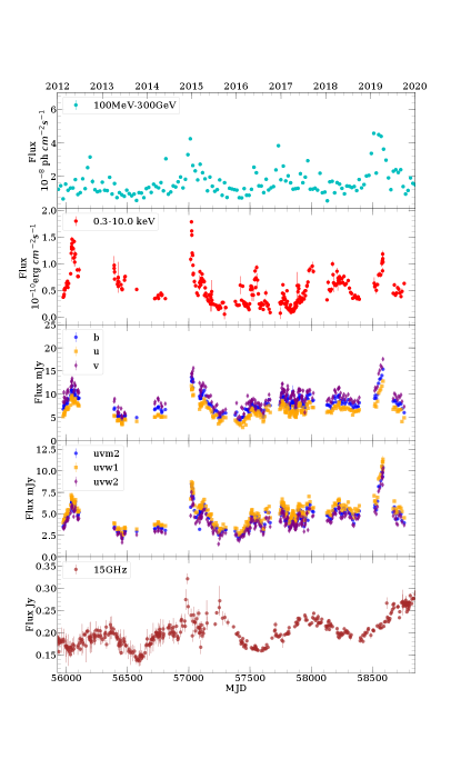
The multi-wavelength light curves during 2012 January – 2020 January of PG 1553+113, ranging from -ray to the radio, are shown in Figure 1. The light curve of -ray exhibits the quasi-periodic variations which were reported by Ackermann et al. (2015). Some weak flares can be seen near the main flares on the -ray light curve. Similar situations can also be seen in the X-ray and optical/UV bands.
When the main flare in the -ray light curves was observed, the prominent outbursts in both X-ray and optical/UV bands could be seen, and, in addition, similar to the case of the -ray, some distinct flares in X-ray and optical/UV bands were observed when the weak flares in -ray were recorded.
In the radio light curve, a quasi-periodic variation can also be seen, however, weak flares are not observed clearly.
4 Discussion
The quasi-periodic variation in the -ray light curve of PG 1553+113 was explained by the jet precession in the SMBHB (Caproni et al., 2017). One-jet model is appropriate for main flares, while the existence of the weak peaks on the light curve, possibly requires a two-jet model to explain this phenomenon (see e.g., Tavani et al. 2018, Cavaliere et al. 2019).
We attempted to fit the X-ray light curves with the single jet precession, but unfortunately, the obtained period is much shorter than that in the case of -ray when the same model was used for fitting. Moreover, similar behavior of the main and weak flares in the correlation between flux and spectral index may be the signature of two jets. Based on this possibility, in order to explore the origin of the X-ray outbursts, we propose the two-jet model for this case.
4.1 The two-jet precession model
In this model, a SMBHB system is considered and each black hole carries its own jet and the movement of the black holes on the orbit causes the quasi-periodic variation on the light curves (Villata et al., 1998; Tavani et al., 2018).
Motivated by the work of Villata et al. (1998), we obtain a function of the angle between the line of sight and the jet direction
| (1) | |||||
| (2) |
where the subscripts 1 and 2 correspond to the first and the second jet, respectively, and , are the angles between the line of sight and the jet direction, and are the angles between the line of sight and the orbital angular momentum/spin of the individual black hole (assuming that the spin parallel to the orbital angular momentum), and are the angles between the orbital angular momentum and the jet direction, is the orbital angular velocity and is the phase position.
The flux of the jet can be expressed as , where is the flux in the rest frame, and is the Doppler factor which can be written as , where is the bulk velocity and is the Lorentz factor. In addition, before fitting, we transform the flux into luminosity through , where is the luminosity distance. In our model, the observed luminosity can be obtained as
| (3) |
where and are the luminosity of jet 1 and jet 2, the subscript 1, 2 of refers to the Doppler factor of the two jets, and is the contribution from other sources such as the disc, corona, etc. For simplification, the precession of the disc, gravitational redshift, and intrinsic variety of accretion flow is not considered here, therefore, for convenience, we assume that is not a time-dependent physical quantity in our model.
4.2 Fitting results
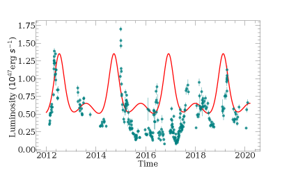
In the fitting, we only fixed the orbital angular velocities () of both black holes. To be consistent with the case of -ray, the period was frozen as . Additionally, was frozen as which is the minimum value in the light curve. Meanwhile, with assumption , other parameters in the model were freed. However, Villata et al. (1998) assumed the two jets share the same values of the parameters when they tried to explain the quasi-periodic double peak structure in the optical light curves of OJ 287. In our work, we do not set the parameters of the two jets (except for the orbital angular velocities and ) to be equal. The Markov Chain Monte Carlo (MCMC) emcee package (Foreman-Mackey et al., 2013) was used in the fitting and 500 walkers and 10000 steps were run666The chain was accessed by using the EnsembleSampler.get_chain in python package emcee. Within this method, we obtained the parameter values as a function of the step numbers in the chain. When the parameters do not change much, the chain can be considered stable. . We adopt the uniform prior as , , , , . The fitted result is shown in Figure 2. More details for the fitted parameters in our model are shown in Table 1.
The fitting is unsatisfactory, with a reduced chi-square of 348.41. However, we did not expect a perfect result based on the X-ray light curve, mainly because of the simple model and the lack of continuous observations for this object. Nevertheless, we had tried to free the period parameter in the fitting, but in the results, the fitted period of 2.8 years is inconsistent with the case of -ray (Ackermann et al., 2015). Tavani et al. (2018) showed the consistency between the R-band and X-ray light curves in the long-term observations. Additionally, Sandrinelli et al. (2018) and Tavani et al. (2018) reported a similar behavior in the long-term -ray and the R-band light curve. Therefore, we can assume that the -ray and X-ray light curves are correlated to some extent. Hence, in fitting, it is reasonable to fix the periodicity to 2.2 years from continuously monitoring -ray data (Caproni et al., 2017; Sandrinelli et al., 2018; Cavaliere et al., 2019).
As mentioned in the last subsection, we only consider the geometric effect in the system in this work. The profile of the X-ray light curve of PG 1553+113 is fairly complicated, while the fitted model in this work is rather simple and it can not describe all the data points in the X-ray. We have tried to improve the model to fit the X-ray light curve and some geometric effects were considered in the test. Although the statistical fitting result is slightly improved, the data sampling still plays an important role. The sparse sample can be fitted well by such complex models may not indicate the true nature of the system. To further investigate the detail of the variability, more high cadence observations are needed. The origin of the X-ray is very complex and there exist some other mechanisms that would modulate the variability. Based on the assumption that the quasi-periodic variation in the X-ray light curve is origin from the emission of the jets, we only explore the effect of the two jets’ precession. However, according to Sobacchi et al. (2017), the Lense-Thirring precession would modulate the oscillation of angle with the time scale from days to years and this may affect on the X-ray variability. Additionally, we did not consider the intrinsic variation of the jets, so our model can not mirror the activity in the jets. For these reasons, the predicted light curve may not fit the observed data very well.
Although the data points in the light curve can not be described well by the two-jet precession scenario, the main and weak flares can be explained well. In order to predict variability accurately, more aspects need to be taken into account. However, in this work, we mainly focus on the effect caused by the precession of two jets in the SMBHB system.
| Parameter | Value | Parameter | Value |
|---|---|---|---|
| 4.35 degree | 2011.40 | ||
| 1.66 degree | 2.64 degree | ||
| 7.67 | 11.96 | ||
| 176.59 degree |
Note. — We obtain the fitting results with the two-jet model through emcee. The subscripts 1 and 2 correspond to the parameter of the jet 1 and jet 2. is the reference time.
4.3 The mass estimation of each black hole
The mass of each black hole was not directly estimated in the previous investigations. We can only constrain the orders of magnitude of the two black holes masses through the fitting results. Following the relation between the power of jets and the luminosity of the discs, the mass of each black hole can be estimated. According to Ghisellini et al. (2014),
| (4) |
where is the radiative power of the jet, and is the disc luminosity. Assuming that X-ray originated from synchrotron emission, the radiative power of the jet can be written as
| (5) |
where is the bolometric luminosity of the jet which can be estimated following the method of Runnoe et al. (2012).
Substituting the fitting results from Table 1 into Equations (5) and (4), and assuming the accretion rate as 0.1 (following Ackermann et al., 2015), where is the Eddington accretion rate, we obtain the masses of the black holes launching jet 1 and jet 2 are and , respectively. The inferred mass ratio is that is in agreement with Tavani et al. (2018). The total mass of the SMBHB system is consistent with the results of Ackermann et al. (2015) and Cavaliere et al. (2019).
4.4 The X-ray properties evolution
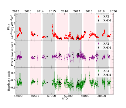
The X-ray energy spectra were analyzed with the redshift power-law model (zpowerlw) through xspec version 12.10.1f. The mean value of the power-law index is with the maximum and minimum value of and respectively, and the results can be seen on the middle panel of Figure 3. Centering at the peak time, we define the 80% of the interval between the two predicted time of minimum luminosity as the flare epoch. We can also define three states to describe the X-ray activity: quiescent, weak flares, and main flares, which corresponding to the different epochs in the results of the two-jet precession model.
To study the evolution of the X-ray flux of PG 1553+113, we analyzed the hardness ratio (HR) expressed as
| (6) |
where CR(2.0–10.0 keV) and CR(0.3–2.0 keV) are counts rate of the hard and soft X-ray, respectively. The evolution of HR is shown on the bottom panel of Figure 3. From 2012.0 to 2020.0, the average value of HR is with the maximum and minimum value are and respectively, which exhibits a very soft level in the stage.
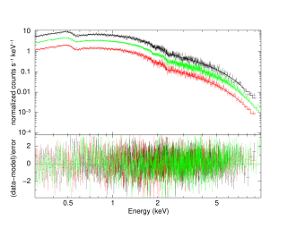
We analyse X-ray data acquired by the XMM-Newton Observatory. The main flare spectrum was obtained in September 6, 2001 (ID 0094380801), the weak flare was observed in July 24, 2013 (ID 0727780101), and the spectrum for a quiescent state with observation ID 0810830201 was obtained in August 27, 2019. The spectra were analysed with xspec, and final results are presented in Figure 4. The X-ray energy spectra exhibit different behavior at these epochs. Raiteri et al. (2015) compared the spectral energy distribution (SEDs) for three states, and from their results, the quiescent state SEDs showed the significant different behavior from the flare states in -ray, which may be the contribution of the jet’s activity.
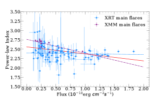
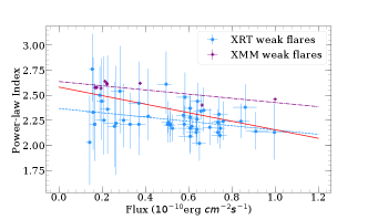
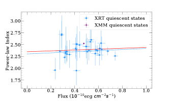
4.5 Flare spectral indices
The power-law index and hardness ratio stay at a relatively stable level most of the time. The best linear fit of the correlation between flux and the power-law index are shown in Figure 5, and the results reveal a slightly “harder-when-brighter” feature during the main and weak flares while for the quiescent state, the slightly “softer-when-brighter” tendency can be seen. We explore the correlation between the index and flux with Spearman test. The analysis is processed by the python package scipy.stats.spearmanr. During main flares, the correlation coefficients () for all cases with p-value . For the case of weak flares, and the p-value (the result from XMM-Newton shows the p-value of 0.675). The result of quiescent state reveals with p-value . It should be noted that in the quiescent state, we obtain only one data point from XMM-Newton, hence the correlation test for this instrument can not be applied. More details for the linear fitting and Spearman test are shown on Table 2.
When we fit all the data together, the slop is very different from the separated fitting results. We note that this behavior is related to the distribution of data points. 8 XMM data points for weak flares locate on the low flux and the power-law index . And for the case of XRT, few points locate on such interval. Therefore, the XMM data points decrease the slope when we fit the data from two instruments together.
The similar evolution of the spectral index for both main and weak flares suggest the same radiation mechanism, which may be related to the jets. The different behavior of the quiescent states and flares may be the contribution of the precession of jets. When the jet pointing to the observer, the “harder-when-brighter” tendency in the flares states can be seen, and in the quiescent state, with the fraction of the contribution from the disc increase, the spectra tend to be “softer-when-brighter” (Wang & Jiang, 2020).
| Epoch | Instrument | P-Value | Slope | Intercept | |
|---|---|---|---|---|---|
| Main flares | XRT | -0.296 | 0.003 | ||
| Main flares | XMM | -0.846 | 0.001 | ||
| Main flares | All | -0.406 | |||
| Weak flares | XRT | -0.308 | 0.033 | ||
| Weak flares | XMM | -0.152 | 0.675 | ||
| Weak flares | All | -0.415 | 0.001 | ||
| Quiescent state | XRT | 0.107 | 0.567 | ||
| Quiescent state | XMM | - | - | - | - |
| Quiescent state | All | 0.105 | 0.566 |
Note. — The Spearman-rank test correlation coefficient, p-value, slope, intercept, respectively. The slope and intercept are obtained from the linear fitting. We compare the results of two instruments for each epoch. Then, the data of Swift and XMM-Newton are combined together in the analysis and the results are shown on the rows labeled with “All”.
4.6 Some possible origins for X-ray light curves variation
In the previous subsections, we argue that the X-ray variation is dominated by the precession of jets, however, the other potential contributions may be considered. We discuss the lighthouse effect, general relativity effect, disc instability, and Lense-Thirring precession below. But the timescale of the variation from these effects is inconsistent with the 2.2-year quasi-periodicity, however, we can not exclude out the modulation of these effects on the long and short timescale variability of PG 1553+113.
4.6.1 The lighthouse effect
With the magnetic field of the disc, the plasma bubbles may be injected into the jet and would be forced to move along it. As the result, the rotation of these bubbles around the jet would induce the variability of the light curves (Camenzind & Krockenberger, 1992). In this scenario, the variation of the light curves is determined by the viewing angle between the line of sight and the velocity direction of the bubbles and the angle should be time-dependent and is related to the spin of the black hole. The lighthouse effect can explain the intraday variability of 3C 273 and BL Lacertae well. However, the variability timescale of this effect is shorter compared to the quasi-periodicity of 2.2-year in PG 1553+113.
4.6.2 General relativity effect on the jet
When a blob is produced and propagate from disc to jet, its motion would be affected by the magnetic field, the radiation field, and the gravitational field which may induce the variation of the light curves (Abramowicz et al., 1990; Mohan & Mangalam, 2015). According to this scenario, the production of a blob is located in the vicinity of the black hole, as a result, some general relativity (GR) effects such as the gravitational redshift, gravitational lensing and the time delay should be taken into account. The helical orbit of the blobs cause the quasi-periodic variation of the light curves, and the results of Mohan & Mangalam (2015) suggest that its time scale ranges from few days to tens of days.
4.6.3 Disc instability
The whole SMBHB system may be surrounded by a huge disc so that the two black holes are embedded in it, and the periodic leakage of the gas into the cavity around the SMBHB may occur (Tanaka, 2013). As a result, the fluctuation of flux which is produced by the periodic accretion can be observed. In this scenario, the variation time scale is related to the orbital period, however, the X-ray emission should be very soft and its light curve would decline as a power-law just similar to the case of tidal disruption events (). According to the fitting results, the emission of PG 1553+113 should be dominated by the jets, and the contribution of the disc is weaker at least by an order of magnitude. Hence we argue that the effect of the instability of the disc may be inconspicuous for PG 1553+113.
4.6.4 Lense-Thirring precession
The Lense-Thirring precession of the disc would induce the quasi-periodic oscillations (QPO) in the Kerr space time (Aschenbach, 2004; Johannsen & Psaltis, 2011). For the case of PG 1553+113, the time scale of QPO due to Lense-Thirring precession is much longer than the orbital period in SMBHB system (Sobacchi et al., 2017). As a consequence, the effect from the Lense-Thirring precession only contributes to the long time scale period of this system.
5 Conclusion
Blazar PG 1553+113 is a SMBHB system candidate showing quasi-periodic variability across the electromagnetic spectrum. The physical origin of this variability is still not well-understood. We study the flux and spectral variability of PG 1553+113 on long-term timescales using Swift and XMM-Newton X-ray data collected for the period 2012–2020. During this period, the X-ray light curve of PG 1553+113 exhibits several main and weak flares. The main X-ray flares and some weak flares are consistent with the corresponding flares observed on the -ray band. A “harder-when-brighter” behavior is observed in the X-ray for both main and weak flares, while a “softer-when-brighter” behavior in quiescent states.
The observed quasi-periodic variation in the -ray light curves could be explained with one-jet model, however the origin of weak X-ray flares would remain unclear. In this study, we apply a two-jet model and show that the contribution from another jet and the accretion disc should be considered to explain the X-ray variability. Based on our fitting results for the X-ray light curve and the correlation between the disc and the jet (Ghisellini et al., 2014), we obtain the mass of the primary black hole is , the secondary one , and the mass ratio that is in line with previous studies. Although we can not obtain the exact values of the parameters, the order of magnitude of the total mass and the mass ratio are consistent with the previous works. In order to research the more detail of the variability, more high cadence observations are needed.
Blazar PG 1553+113 is not the first object with possible double-jet structure signatures. For example, Qian et al. (2019) proposed a double-jet structure scenario for 3C 279 and suggested that there may be a SMBHB ejecting two precessing relativistic jets. At variance with their method, we focused on X-ray bands. This may be a indirect tool to search such SMBHB systems with two jets in the future.
In the extreme mass ratio black hole binary systems, the accretion disc may not form around the secondary black hole within the gravity of the primary one, such as OJ 287 (Lehto & Valtonen, 1996). However, in mildly mass ratio SMBHB systems, it is possible that each black hole may have its own disc (Farris et al., 2014; Bowen et al., 2017; Ryan & MacFadyen, 2017) and two-jet signature can be detected. Probably, our approach is valid in the case of the SMBHB systems with a mild mass ratio and we can detect such types of black hole systems in the future.
In complex environment of blazars, a pure geometric model is one of the tools to study the X-ray light curves. A simple model should not be expected to complete the explanation perfectly. Some intrinsic variation in the jets and discs should be considered in further research.
References
- Abraham & Carrara (1998) Abraham, Z. & Carrara, E. A. 1998, ApJ, 496, 172
- Abraham & Romero (1999) Abraham, Z. & Romero, G. E. 1999, A&A, 344, 61
- Abraham (2000) Abraham, Z., 2000, A&A, 355, 915
- Abramowicz et al. (1990) Abramowicz, M. A., Ellis, G. F. R., & Lanza, A. 1990, ApJ, 361, 470
- Ackermann et al. (2015) Ackermann, M., Ajello, M., Albert, A., et al. 2015, ApJ, 813, L41
- Aschenbach (2004) Aschenbach, B. 2004, A&A, 425, 1075
- Astropy Collaboration et al. (2013) Astropy Collaboration, Robitaille, T. P., Tollerud, E. J., et al. 2013, A&A, 558, A33
- Astropy Collaboration et al. (2018) Astropy Collaboration, Price-Whelan, A. M., Sipőcz, B. M., et al. 2018, AJ, 156, 123
- Atwood et al. (2009) Atwood, W. B., Abdo, A. A., Ackermann, M., et al. 2009, ApJ, 697, 1071
- Bowen et al. (2017) Bowen, D. B., Campanelli, M., Krolik, J. H., et al. 2017, ApJ, 838, 42
- Britzen et al. (2018) Britzen, S., Fendit, C., Witzel, G., et al. 2018, MNRAS, 478, 3199
- Burrows et al. (2005) Burrows, D. N., Hill, J. E., Nousek, J. A., et al. 2005, Space Sci. Rev., 120, 165
- Camenzind & Krockenberger (1992) Camenzind, M., & Krockenberger, M. 1992, A&A, 255, 59
- Caproni et al. (2017) Caproni, A., Abraham, Z., Motter, J. C., et al. 2017, ApJ, 851, L39
- Cavaliere et al. (2017) Cavaliere, A., Tavani, M., & Vittorini, V. 2017, ApJ, 836, 220
- Cavaliere et al. (2019) Cavaliere, A., Tavani, M., Munar-Adrover, P., et al. 2019, ApJ, 875, L22
- Covino et al. (2020) Covino, S., Landoni, M., Sandrinelli, A., et al. 2020, ApJ, 895, 122
- Dey et al. (2018) Dey, L., Valtonen, M. J., Gopakumar, A., et al. 2018, ApJ, 866, 11
- Farris et al. (2014) Farris, B. D., Duffell, P., MacFadyen, A. I., et al. 2014, ApJ, 783, 134
- Foreman-Mackey et al. (2013) Foreman-Mackey, D., Hogg, D. W., Lang, D., et al. 2013, PASP, 125, 306
- Ghisellini et al. (2014) Ghisellini, G., Tavecchio, F., Maraschi, L., et al. 2014, Nature, 515, 376
- Hunter (2007) Hunter, J. D. 2007, Computing in Science and Engineering, 9, 90
- Johannsen & Psaltis (2011) Johannsen, T., & Psaltis, D. 2011, ApJ, 726, 11
- Katz (1997) Katz, J. I., 1997, ApJ, 478, 527
- Laine et al. (2020) Laine, S., Dey, L., Valtonen, M., et al. 2020, ApJ, 894, L1
- Lehto & Valtonen (1996) Lehto, H. J., & Valtnoen, M. J., 1996, ApJ, 460, 207
- Mohan & Mangalam (2015) Mohan, P., & Mangalam, A. 2015, ApJ, 805, 91
- Qian et al. (2019) Qian, S. J., Britzen, S., Krichbaum, T. P., et al. 2019, A&A, 621, A11.
- Raiteri et al. (2015) Raiteri, C. M., Stamerra, A., Villata, M., et al. 2015, MNRAS, 454, 353
- Richards et al. (2011) Richards, J. L., Max-Moerbeck, W., Pavlidou, V., et al. 2011, ApJS, 194, 29
- Roming et al. (2005) Roming, P. W. A., Kennedy, T. E., Mason, K. O., et al. 2005, Space Sci. Rev., 120, 95
- Runnoe et al. (2012) Runnoe, J. C., Brotherton, M. S., & Shang, Z. 2012, MNRAS, 422, 478
- Ryan & MacFadyen (2017) Ryan, G. & MacFadyen, A. 2017, ApJ, 835, 199
- Sandrinelli et al. (2018) Sandrinelli, A., Covino, S., Treves, A., et al. 2018, A&A, 615, A118
- Sobacchi et al. (2017) Sobacchi, E., Sormani, M. C., & Stamerra, A. 2017, MNRAS, 465, 161
- Tanaka (2013) Tanaka, T. L. 2013, MNRAS, 434, 2275
- Tavani et al. (2018) Tavani, M., Cavaliere, A., Munar-Adrover, P., et al. 2018, ApJ, 854, 11
- Urry & Padovani (1995) Urry, C. M., & Padovani, P. 1995, PASP, 107, 803
- Valtonen et al. (2008) Valtonen, M. J., Lehto, H. J., Nilsson, K., et al. 2008, Nature, 452, 851
- Valtonen et al. (2016) Valtonen, M. J., Zola, S., Ciprini, S., et al. 2016, ApJ, 819, L37
- Villata et al. (1998) Villata, M., Raiteri, C. M., Sillanpaa, A., et al. 1998, MNRAS, 293, L13
- Virtanen et al. (2020) Virtanen, P., Gommers, R., Oliphant, T. E., et al. 2020, Nature Methods, 17, 261.
- Wang & Jiang (2020) Wang, Y.-F. & Jiang, Y.-G. 2020, ApJ, 902, 41.
- Yan et al. (2018) Yan, D., Zhou, J., Zhang, P., et al. 2018, ApJ, 867, 53
- Zhou et al. (2018) Zhou, J., Wang, Z., Chen, L., et al. 2018, Nature Communications, 9, 4599