Theoretical Approaches to Liquid Helium

Liquid Helium was first liquefied by Kammerlingh Onnes in 1908 (Kamerlingh Onnes, 1908) and, since then, it has been one of the most studied quantum systems. Two of its isotopes are stable, ⁴He and ³He. In naturally produced Helium, the fraction of ³He is extremely small, 1 part in 10⁶, and is produced from radioactive decay of tritium. Both isotopes remain in liquid state even in the limit of zero temperature, manifesting in this way their intrinsic quantum nature. Contrarily to classical theory, that predicts that any material becomes solid in that limit, quantum mechanics explain this fail of the classical approach by considering the zero-point kinetic energy. The combination of the light mass of Helium atoms and their weak attraction produces the unique opportunity of observing the most paradigmatic quantum liquid. ⁴He and ³He have different masses but the most crucial difference between both isotopes affects their behavior as quantum many-body systems: ⁴He is composed by an even number of spin $1/2$ particles and thus, it is a boson, whereas ³He has an odd number of constituents and behaves as a fermion. As we will discuss in this article, the different quantum statistics of the two Helium isotopes produces dramatic differences between them.

In ⁴He, the specific heat shows a large excess at a temperature of $2.17$ K, signaling the emergence of a phase transition, first observed by Keesom and Clusius (Keesom and Clusius, 1932). The specific heat shows a shape similar to the $\lambda$ Greek letter and is now universally known as the $\lambda$ phase transition, with a critical temperature $T_{c}=2.17$ K. This second-order transition separates two liquids with different properties and were termed liquid He I and liquid He II for $T>T_{c}$ and $T<T_{c}$, respectively. In 1937, P. Kapitza (Kapitza, 1938), from one side, and J. F. Allen and A. D. Misener (Allen and Misener, 1938), on the other, published back to back papers announcing the discovery of superfluid ⁴He in the Helium II phase. For an insightful historical analysis of the role played by the two independent teams on that discovery, we recommend the paper by Balibar (Balibar, 2007). Below $T_{\lambda}$, ⁴He flows with vanishingly small viscosity producing a set of surprising effects such as the fountain effect, absence of boiling due to the large thermal conductivity, second sound, etc. (Wilks, 1967).

In the early theoretical approaches to understand the extraordinary behavior of liquid Helium around the $\lambda$ point, four names appear above many others: Laszlo Tisza, Lev Landau, Fritz London and Nikolai Bogoliubov. Tisza and Landau worked in a quantum hydrodynamic approach with the main idea of Helium as a liquid composed by two independent liquids (velocity fields). This is the basis of the two-fluid model first introduced by Tisza (Tisza, 1938) and then completed by Landau (Landau, 1941). The two-fluid model assumes that the total density is the sum of two partial densities: the normal and the superfluid. Below $T_{\lambda}$, the superfluid component dominates, thus explaining the superfluid properties of Helium II. Increasing the temperature, at $T\geq T_{\lambda}$, the superfluid density turns to be zero and the total density equals the normal one.

Landau (Landau, 1941) introduced the concept of quasiparticle to postulate the shape of the excitation spectrum. Instead of single-particle excitations, the system presents collective modes that at low momenta are termed phonons, in resemblance with the excitation spectrum of a crystal. At low momenta, the excitations are linear with the momenta, the slope being the speed of sound. At larger momenta, Landau defined another type of collective excitations which were named rotons, since where initially related to the presence of quantized vortices. Landau predicted that below a certain velocity, termed critical velocity, the system cannot be excited and thus liquid Helium flows without friction. Combining phonons and rotons, Landau (Landau, 1947) was able to draw the excitation spectrum of Helium before any measure of it was made.

The hydrodynamic theory by Tisza and Landau did not take into account the quantum statistics of ⁴He because they believed that this feature was not relevant to understand the superfluidity and the $\lambda$ phase transition. On the contrary, London (London, 1938) argued that a Bose gas experiences a second-order phase transition that can explain, at least qualitatively, the $\lambda$ transition in ⁴He. Applying the critical temperature derived in the Bose-Einstein statistics,

$$k_{B}T_{\text{BEC}}=\frac{2\pi\hbar^{2}}{m}\,\left(\frac{n}{g_{3/2}(1)}\right)^{2/3}\ ,$$

(1)

with $g_{3/2}(1)\simeq 2.612$ and $n$ the density, to the case of Helium London obtained $3.1$ K, not so far from $T_{\lambda}$. Landau always ignored London approach to the problem (Balibar, 2007) because with his hydrodynamic theory he was able to account for many experimental facts. However, we know now that the quantum statistics of ⁴He is crucial to understand superfluid ⁴He. When samples of ³He were produced, we learned that ³He, which is a fermion, do not show the $\lambda$ phase transition.

Bogoliubov, in 1947 (Bogoliubov, 1947), was the first to connect the elementary excitation spectrum with a Bose-Einstein gas with repulsive but small interatomic interaction. He proved that the lowest-energy excitations are collective modes (phonons) that at low momenta are proportional to the speed of sound, in agreement with Landau theory. The Bogoliubov excitation spectrum (Pitaevskii and Stringari, 2016)

$$\varepsilon(p)=\left[\frac{gn}{m}p^{2}+\left(\frac{p^{2}}{2m}\right)^{2}\right]^{1/2}\ ,$$

(2)

with $g$ the interaction strength, predicts a critical velocity which is always equal to the speed of sound. Bogoliubov theory was again qualitatively correct but Helium is not a rarefied gas but a liquid with strong interparticle interactions.

We discuss first liquid ⁴He, ³He was obtained later in time due to its complex experimental production. As we commented in the previous Section, Bogoliubov (Bogoliubov, 1947) introduced field theoretical models in the theoretical description of liquid ⁴He, but his approach was only applicable to dilute Bose gases and this is far form the real properties of Helium. This is specially evident from the explicit assumption in Bogoliubov analysis that all the particles of the system are in the Bose-Einstein condensate, whereas in ⁴He only  7% of them are really in this state due to the unavoidable role played by atomic correlations. In subsequent work, Beliaev (Beliaev, 1958) introduced Green functions $G_{\alpha,\beta}(q,\omega)$ in the formalism, deriving a general equation for them at zero temperature. The quantum field theory for a Bose fluid was reanalyzed by Hugenholtz and Pines (Hugenholtz and Pines, 1959) by the introduction of the chemical potential $\mu$ to guarantee the number conservation of the theory. Importantly, they removed the constraint of a full condensate, approaching better the characteristics of liquid Helium. An important result of this approach was the calculation of the energy of a Bose gas incorporating the first corrections to the Hartree-Fock energy

$$\frac{E}{N}=4\pi na^{3}\left[1+\frac{128}{15\sqrt{\pi}}\sqrt{na^{3}}+\frac{8(4\pi-3\sqrt{3})}{3}na^{3}\ln(na^{3})+\ldots\right]\ ,$$

(3)

the energy per particle $E/N$ being in units of $\hbar^{2}/(2ma^{2})$. Hugenholtz and Pines (Hugenholtz and Pines, 1959) proved that, beyond the expansion terms in Eq.(3), additional contributions will depend on the specific shape of the interatomic potential and not only on the $s$-wave scattering length $a$. The coefficient of the $(na^{3})^{3/2}$ term was first calculated by Lee, Huang and Yang (Lee, Huang and Yang, 1957), while the coefficient of the last term was first obtained by Wu (Wu, 1959). Both of them were originally derived for hard spheres, but it was shown that the same expansion is valid for any repulsive potential with scattering length $a$ (Hugenholtz and Pines, 1959). Equation (3) has been very useful in the study of dilute Bose gases, composed by alkali atoms, due to their extreme diluteness (Pitaevskii and Stringari, 2016). However, liquid Helium is a strongly interacting quantum many-body system in which any expansion in terms of the gas parameter $na^{3}$ is completely useless.

The first theoretical approach based on the wave function of the $N$-body quantum system was made by Feynman (Feynman, 1953). This work opened a new way to deal with the properties of Helium based on a microscopic approach. Starting from general arguments, that included the symmetry of the ⁴He atoms and their hard-core interactions at short distances, Feynman argued that the lowest-energy excitations have a collective behavior since single-particle ones have always higher energy. Based on these considerations, he wrote the wave function of the excited state of the $N$-body fluid as

$$\Psi(\bm{r}_{1},\ldots,\bm{r}_{N})=\prod_{i=1}^{N}f(\bm{r}_{i})\ \Phi(\bm{r}_{1},\ldots,\bm{r}_{N})\ ,$$

(4)

with $\Phi(\bm{r}_{1},\ldots,\bm{r}_{N})$ the ground-state wave function. Equation (4) is a variational approach to the problem and thus the energy of the excitation is an upper bound to the exact energy. He obtained the lowest excitation energy

$$\hbar\omega_{\text{F}}(q)=\frac{\hbar^{2}q^{2}/2m}{S(q)}\ ,$$

(5)

with $S(\bm{q})=1/N\langle\rho^{\dagger}(\bm{q})\rho(\bm{q})\rangle$ the static structure factor, $\rho(\bm{q})=\sum_{i}\exp(-i\bm{q}\cdot\bm{r}_{i})$ being the density fluctuation operator. When $\bm{q}\to 0$, $S(q)=\hbar q/(2mc)$, with $c$ the speed of sound. In this way, Feynman recovers the phonon relation previously found by Landau and Bogoliubov, $\hbar\omega=cq$, that is, a linear behavior. At large momenta, the static structure factor tends to 1 and so one recovers the excitation energy of a free particle $\hbar^{2}q^{2}/2m$, quadratic with $q$. At intermediate $q$ values, $S(q)$ shows a peak related to the mean interparticle distance and thus the excitation energy (5) shows a local minimum that we can identify with the roton. Qualitatively, the Feynman spectrum is correct up to momenta not much larger than the one of the roton but the roton energy is nearly two times larger than the experimental one. The minimum energy (5) is obtained with a function $f(r)=\exp(i\bm{q}\cdot\bm{r})$, so the total wave function (4) is given by

$$\Psi(\bm{r}_{1},\ldots,\bm{r}_{N})=\prod_{i=1}^{N}e^{i\bm{q}\cdot\bm{r}_{i}}\ \Phi(\bm{r}_{1},\ldots,\bm{r}_{N})=\rho^{\dagger}(\bm{q})\Phi(\bm{r}_{1},\ldots,\bm{r}_{N})\ ,$$

(6)

that emerges as the creation of a collective mode of momentum $\bm{q}$ acting on the ground-state, that is not changed by the excitation.

Feynman and Cohen (Feynman and Cohen, 1956) improved the initial theory by introducing in the wave function two-body correlations. Their idea is that when one particle moves in the fluid its neighbors feel the movement or, in other words, the movement of each particle depends on its local environment. They termed these correlations as backflow correlations. Explicitly, the wave function of the collective excitation turns to

$$\Psi(\bm{r}_{1},\ldots,\bm{r}_{N})=\prod_{i=1}^{N}\left[e^{i\bm{q}\cdot\bm{r}_{i}}\sum_{j\neq i}e^{ig(\bm{r}_{i}-\bm{r}_{j})}\right]\Phi(\bm{r}_{1},\ldots,\bm{r}_{N})\ .$$

(7)

The function $g(r)$ in Eq. (7) couples the movement of the excited particle $i$ with the neighboring ones. In Ref. (Feynman and Cohen, 1956), it is taken as a dipolar term, $g(r)=\alpha\bm{q}\cdot\bm{r}/r^{3}$ and the imaginary exponential containing $g(r)$ is linearized to make the calculation of the energy simpler. With this correction, the difference between the Feynman roton energy (5) and the experimental one is reduced in a factor $\sim 2$ but still there is a significant difference.

To reproduce as better as possible the elementary excitation spectrum of liquid ⁴He is not the only goal of a microscopic theory. It is fundamental to have an accurate description of the ground state of the system. The most fruitful approach to account for the equation of state of liquid ⁴He has been the variational theory since standard perturbative approaches are not applicable due to the hard-core of the He-He interaction at short distances. The Hamiltonian of the $N$-particle system is

$$H=-\frac{\hbar^{2}}{2m}\sum_{i=1}^{N}\bm{\nabla}_{i}^{2}+\sum_{i<j}^{N}V(r_{ij})\ ,$$

(8)

with $V(r)$ the pair interatomic potential. One can add to Eq. (8) three-body potentials, whose analytic form is not well known. However, its contribution to the energy seems to be not relevant and the results can even worsen (Boronat and Casulleras, 1994). In the description of the bulk phases, one always assumes the thermodynamic limit: $N\to\infty$, $\Omega\to\infty$, and the density $\rho=N/\Omega$ is finite. For a trial wave function $\Psi$, not orthogonal to the ground state, the Ritz’s variational principle of quantum mechanics states that

$$E=\frac{\langle\Psi|H|\Psi\rangle}{\langle\Psi|\Psi\rangle}\geq E_{0}\ ,$$

(9)

with $E_{0}$ the ground-state energy of the system. The wave function $\Psi$ must be symmetric under the interchange of particles and approaches zero when $r_{ij}\to 0$. Also, when a set of particles is significantly far way from the rest of the system the total wave function factorizes, i.e., the cluster property is fulfilled. The first model wave function that comes to mind is a symmetrized product of single-particle wave functions which, for a bulk phase, are plane waves. However, this model clearly violates both crucial properties. Bijl (Bijl, 1940) and Jastrow (Jastrow, 1955) proposed a model to account with the restrictions imposed by a strongly correlated fluid,

$$\Psi(\bm{r}_{1},\ldots,\bm{r}_{N})=\prod_{i=1}^{N}g(r_{i})\,\prod_{i<j}^{N}f(r_{ij})\ ,$$

(10)

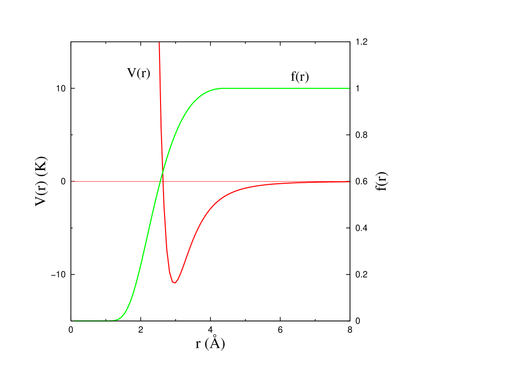
with $f(r)$ a two-body correlation factor and $g(r)$ a one-body function that, in the bulk phase, is simply 1 (ground-state). The function $f(r)$ plays an essential role in the study of Helium and satisfies two main properties: it becomes zero, approaching the hard-core of the potential, and one at large distance, according to the cluster property. In Fig.1, we show the characteristic shape of the potential and the two-body correlation factor.

The energy per particle for a Bijl-Jastrow wave function is readily obtained as

$$\frac{E}{N}=\frac{1}{2}\rho\int d\bm{r}\left[V(r)-\frac{\hbar^{2}}{2m}\bm{\nabla}^{2}\ln f(r)\right]\ ,$$

(11)

with $g(r)$ the two-body radial distribution function

$$g(r_{12})=\frac{N(N-1)}{\rho^{2}}\frac{\int d\bm{r}_{3}\ldots d\bm{r}_{N}|\Psi(\bm{r}_{1},\ldots,\bm{r}_{N})|^{2}}{\int d\bm{r}_{1}\ldots d\bm{r}_{N}|\Psi(\bm{r}_{1},\ldots,\bm{r}_{N})|^{2}}\ ,$$

(12)

which is proportional to the probability of finding two particles at distance $\bm{r}$. Accessing to the function $g(r)$ allows for the calculation of the energy of the system and further properties. However, as Eq. (12) shows, its estimation is very difficult due to the multidimensional integrals that need to be carried out. A fruitful approach in the study of liquid Helium has been the hyppernetted chain theory (HNC) based on the summation of the series in terms of the function $h(r)=f^{2}(r)-1$ in which $g(r)$ can be expressed. This function $h(r)$ is different from zero only at short distances and allows for a cluster expansion. $g(r)$ is given exactly by

$$g(r)=f^{2}(r)\,\exp(N(r)+E(r))\ ,$$

(13)

where $N(r)$ and $E(r)$ are functions summing up specific terms of the series, known as nodal and elementary diagrams, respectively. Nodal diagrams can be calculated by solving the HNC integral equation

$$N(r_{12})=\rho\int d\bm{r}_{3}[g(r_{13})-1][g(r_{32})-N(r_{32})-1]\ .$$

(14)

On the contrary, elementary diagrams cannot be summed up and, thus, only approximated in some way (Usmani, Friedman and Pandharipande, 1982; Fabrocini and Rosati, 1982; Clements et al., 1993). Therefore, Eq. (13) cannot be evaluated in an exact and closed form using this theory.

The variational upper bound to the exact energy depends on the trial wave function. One can guess an analytic model for it, with a set of variational parameters to be optimized. Otherwise, one can approach the optimization via a functional derivative, normally written in terms of the two-body distribution function $g(r)$,

$$\frac{\delta E[g(r)]}{\delta g(r)}=0\ ,$$

(15)

with $E[g(r)]$ the energy of the system. This can be written only in terms of $g(r)$ by using Eq. (13),

$$E[g(r)]=\frac{\rho}{2}\int d\bm{r}g(r)V(r)+\frac{\hbar^{2}\rho}{2m}\int d\bm{r}\left[\left(\bm{\nabla}\sqrt{g(r)}\right)^{2}+\frac{1}{4}g(r)\bm{\nabla}^{2}E(r)\right]-\frac{\hbar^{2}}{8m}\frac{1}{2\pi^{3}\rho}\int d\bm{k}k^{2}\frac{(S(k)-1)^{3}}{S(k)}\ .$$

(16)

Imposing the minimization condition (15), one arrives to the Euler-Lagrange differential equation for the optimal correlation (Lantto, Jackson and Siemens, 1977; Kallio and Smith, 1977)

$$-\frac{\hbar^{2}}{m}\bm{\nabla}^{2}\sqrt{g(r)}+(V(r)+W(r))\sqrt{g(r)}=0\ .$$

(17)

This equation needs to be solved iteratively (Jackson, Lande and Lantto, 1979) because the potential $W(r)$ depends on the correlation function. Neglecting the contribution of the elementary diagrams, this induced potential is better written in reciprocal space as

$$\tilde{W}(q)=-\frac{\hbar^{2}q^{2}}{4m}\frac{(S(q)-1)(2S(q)+1)}{S(q)^{2}}\ ,$$

(18)

with $S(q)$ the static structure factor,

$$S(q)=\frac{1}{N}\langle\rho_{\bm{q}}\rho_{-\bm{q}}\rangle=1+\rho\int d\bm{r}e^{i\bm{q}\cdot\bm{r}}(g(r)-1)\ .$$

(19)

At zero temperature, the function $S(q)$ satisfies $S(0)=0$ and shows the phononic behavior at small $q$

$$\lim_{q\to 0}S(q)=\frac{\hbar q}{2mc}\ ,$$

(20)

with $c$ the speed of sound. This behavior at small $q$ produces a long-range behavior of the two-body correlation factor (Feenberg, 1969)

$$\lim_{r\to\infty}f(r)=1-\frac{mc}{2\pi^{2}\hbar\rho r^{2}}\ .$$

(21)

Remarkably, the optimal $f(r)$ obtained from the Euler-Lagrange equation (17) satisfies the phonon behavior (21) (Castillejo et al., 1979), even if the speed of sound that derives form that differs from the experimental one.

At zero temperature, the superfluid fraction of ⁴He is one but the occupation of the zero-momentum state, that is the Bose-Einstein condensate, is significantly smaller than one due to the relevance of correlations. Microscopically, the condensate fraction $n_{0}$, and the momentum distribution in general, can be calculated through the one-body density matrix

$$\rho(r_{11^{\prime}})=\Omega\,\frac{\int d\bm{r}_{2}\ldots d\bm{r}_{N}\Psi(\bm{r}_{1},\ldots,\bm{r}_{N})\Psi(\bm{r}_{1^{\prime}},\ldots,\bm{r}_{N})}{\int d\bm{r}_{1}\ldots d\bm{r}_{N}|\Psi(\bm{r}_{1},\ldots,\bm{r}_{N})|^{2}}\ ,$$

(22)

normalized as $\rho(0)=1$. Fourier transforming $\rho(r)$ one gets the momentum distribution

$$n(q)=n_{0}\delta(q)+\rho\int d\bm{r}(\rho(r)-n_{0})e^{i\bm{q}\cdot\bm{r}}\ ,$$

(23)

with $n_{0}=\lim_{r\to\infty}\rho(r)$ the condensate fraction. The momentum distribution (23) can be measured using deep inelastic neutron scattering at large momentum transfer. The condensate fraction is quite small $n_{0}\sim 0.07$ and its estimation, from the dynamic structure factor $S(\bm{q},\omega)$, requires from an accurate analysis of final state effects (Glyde, 1994). A variational estimation of the one-body density matrix and the condensate fraction can be made using a HNC cluster expansion similar to the one developed for $g(r)$ (Fantoni, 1978).

With the best Jastrow factor, the upper bound to the energy provided by the variational calculation is still $~15$% above the exact quantum Monte Carlo results (see next Section) for the same interatomic potential and at densities close to the equilibrium point. An important advance on the improvement of the variational energy was the introduction of three-body correlations in the trial wave function,

$$\Psi_{\text{JT}}(\bm{r}_{1},\ldots,\bm{r}_{N})=\prod_{i<j}^{N}f(r_{ij})\,\prod_{i<j<k}^{N}f_{3}(r_{ij},r_{ik},r_{jk})\ ,$$

(24)

which corrects the description of correlation effects at short and medium interparticle distances. The relevance of these correlations in the study of liquid Helium derives from its relatively large density, which drives this liquid into the realm of one of the most correlated quantum systems in Nature. The origin of the function $f_{3}$, and its specific functional form, can be derived in different ways: introducing a momentum dependence in the two-body correlation factor (Pandharipande, 1978) or by searching the first correction to the Jastrow factor by linearizing the imaginary-time Schrödinger equation (Boronat, 2002). It adopts the form

$$f_{3}(r_{ij},r_{ik},r_{jk})=\exp\left(-\frac{1}{2}\,q(r_{ij},r_{ik},r_{jk})\right)\ ,$$

(25)

where

$$q(r_{ij},r_{ik},r_{jk})=\sum_{l}\sum_{\text{cyc}}\xi_{l}(r_{ij})\xi_{l}(r_{ik})P_{l}(\hat{r_{ij}}\cdot\hat{r_{ik}})\ ,$$

(26)

with $l$ the angular momentum and $P_{l}$ the Legendre polynomial. The most important, and most used contribution, corresponds to $l=1$. The pair function $\xi(r)$ in Eq. (26) is assumed to be a short-range correlation factor

$$\xi(r)=\sqrt{\lambda}\,\exp\left[-\left(\frac{r-r_{t}}{r_{\omega}}\right)^{2}\right]\ ,$$

(27)

with $\lambda$, $r_{t}$, and $r_{\omega}$ variational parameters to be optimized. The HNC equations can be generalized to allow for the inclusion of three-body correlations in the diagrammatic expansions (Usmani, Fantoni and Pandharipande, 1982). The energies obtained so far reduces in a $\sim 70$% the difference between the Jastrow upper bound and the exact values, pointing to its importance for a right microscopic description of liquid ⁴He.

The theoretical description of liquid Helium is not complete without understanding the dynamics of the system. The dynamic structure function $S(\bm{q},\hbar\omega)$ contains the maximum information about it and is experimentally accessible by inelastic scattering through

$$\frac{\partial^{2}\sigma}{\partial\Omega\,\partial\hbar\omega}=b^{2}\left(\frac{q_{1}}{q_{0}}\right)S(\bm{q},\hbar\omega)\ ,$$

(28)

with the left part being the double differential cross section. In Eq. (28), $b$ is the scattering length of the nucleus, and $\bm{q}_{0}$ and $\bm{q}_{1}$ are the initial and final momentum of the neutron. The momentum and energy transferred to the liquid are $\bm{q}=\bm{q}_{1}-\bm{q}_{0}$ and $\hbar\omega$, respectively. At zero temperature, and for a $N$ particle system,

$$S(\bm{q},\hbar\omega)=\frac{1}{N}\sum_{n}|\langle\Psi_{n}|\rho(\bm{q})|\Psi_{0}\rangle|^{2}\delta(\hbar\omega-(E_{n}-E_{0}))\ ,$$

(29)

where the sum is extended to all the excited states and $\rho(\bm{q})$ is the density fluctuation operator. To calculate the dynamic response one invokes linear response theory, where the change in the density under the action of an external tiny time-dependent potential is

$$\delta\rho(\bm{r},t)=\int d\bm{r}^{\prime}dt^{\prime}\chi(\bm{r},\bm{r}^{\prime},t-t^{\prime})\,\delta V_{\text{ext}}(\bm{r}^{\prime},t^{\prime})\ ,$$

(30)

with $\chi$ the density-density response function. The dynamic response can be obtained from the imaginary part of the Fourier transform of $\chi$,

$$S(\bm{q},\hbar\omega)=-\frac{1}{N\pi}\Im\left[\int d\bm{r}d\bm{r}^{\prime}e^{i\bm{q}\cdot(\bm{r}-\bm{r}^{\prime})}\chi(\bm{r},\bm{r}^{\prime},\hbar\omega)\right]\ ,$$

(31)

and the evolution in time of $\delta\rho(\bm{r},t)$ from the least-action principle $\delta S=0$. The calculation of the dynamic response of liquid Helium has been the object of intense work for many years. Regular perturbation theory does not work because of the hard-core of the He-He interaction and then it is necessary to work out the theory using correlated basis functions (CBF). From pioneering work by Feenberg and Jackson (Jackson and Feenberg, 1962) and Lee and Lee (Lee and Lee, 1975), the major progress has been achieved by dynamic many-body theory developed by Krotscheck and Campbell (Campbell and Krotscheck, 2009; Campbell, Krotscheck and Lichtenegger, 2015). Recently, a comparison between very accurate experimental data, on the dynamic response and the excitation spectrum, and theoretical results obtained with dynamic many-body theory has shown an impressive agreement (Beauvois et al., 2018).

Until here, we have focused our discussion on the studies of bosonic liquid ⁴He. But, Helium offers another stable isotope, ³He, which is a fermion. At very low temperatures, it remains in a liquid state that becomes superfluid at $\sim 2$ mK. In the following, we refer to normal non-superfluid ³He since superfluid ³He is a very different subject which would require a completely different scope. The variational wave function incorporates the Fermi statistics in the well-known Jastrow-Slater form

$$\Psi(\bm{r}_{1},\ldots,\bm{r}_{N})=\prod_{i<j}^{N}f(r_{ij})\,\Phi(\bm{r}_{1},\ldots,\bm{r}_{N})\ ,$$

(32)

with $\Phi$ an antisymmetric wave function, usually taken as the product of Slater determinants $\Phi=D_{\uparrow}D_{\downarrow}$ since the interaction is spin independent. Variational theory, based on cluster expansion and summation of proper diagrams, to calculate the pair distribution function $g(r)$ is now more involved than in Bose fluids. The extension of HNC theory is known as Fermi-hypperneted chain (FHNC) and the convergence of the series summation was proved in the seventies of the past century (Fantoni and Rosati, 1975; Krotscheck and Ristig, 1975). This theory was reviewed in depth by Rosati (Rosati, 1981) and a modern update was carried out by Krotscheck (Krotscheck, 2000). As in the case of ⁴He, the inclusion in the trial wave function (32) of triplet correlations reduces significantly the difference with quantum Monte Carlo estimations. Even with the introduction of three body factors into the variational model, the Jastrow-Slater model uses Slater determinants with free single-particle orbitals. A relevant improvement of the variational model is achieved by modifying these orbitals to include, in an approximate way, the effect of correlations on them. This is usually made with backflow correlations, where the orbitals are $\exp(i\bm{k}\cdot\tilde{\bm{r}_{i}})$, with

$$\tilde{\bm{r}_{i}}=\bm{r}_{i}+\lambda\sum_{j\neq i}\eta(r_{ij})\bm{r}_{ij}\ ,$$

(33)

$\eta(r)$ being a short-ranged function as a Gaussian (Manousakis et al., 1983). The calculation of excited states of ³He has also been possible by using CBF theory with increasing complexity due to Fermi statistics (Fabrocini and Rosati, 1988). The high accuracy of CBF theory has been recently proved in a comparison between its predictions and very accurate experimental data on films of ³He (Godfrin et al., 2012).

Working with the two isotopes of Helium, it is also possible to have stable mixtures of ³He and ⁴He, that is a Fermi-Bose mixture. In the limit of zero temperature, the mixture is stable up to a maximum ³He concentration of $~6.5$% (Ebner and Edwards, 1970). This isotopic mixture was first studied neglecting the Fermi character of ³He atoms showing that the isotopic Bose-Bose mixture is not stable at any finite concentration (Chakraborty, 1982). To get realistic results and finite solubilities it is mandatory to consider ³He atoms as fermions. The HNC/FHNC equations were generalized to the mixture by Fabrocini and Polls (Fabrocini and Polls, 1982) and then extended to study the momentum distribution of the mixture (Boronat, Polls and Fabrocini, 1997). The limiting case of a single impurity, known also as polaron, was also studied using HNC/CBF formalism both for the ³He impurity in bulk ⁴He (Boronat, Fabrocini and Polls, 1989) (Bose polaron) and for the ⁴He impurity in ³He (Arias de Saavedra et al., 1994) (Fermi polaron).

Variational methods discussed in the previous Section have been tremendously effective in the description of liquid Helium, with special significance on the accuracy achieved in the calculations of the dynamic response. However, the application of the variational principle guarantees upper bounds to the ground-state energies and it is difficult to know what remains between the bounds and exact values. Quantum Monte Carlo methods exploit the power of stochastic simulations to go beyond the bounds of the variational theories and obtain exact estimations within some statistical noise.

We first discuss the $T=0$ ground state with projection methods. The two methods that have been used in the study of liquid ⁴He are Green’s function Monte Carlo (GFMC) and diffusion Monte Carlo (DMC). GFMC is the most accurate method because it has not any time-step dependence but its implementation is involved. Instead, DMC is a simpler method but with time-step dependence. Nowadays, DMC has become the most used tool.

The DMC method solves the Schrödinger equation, written in imaginary time,

$$-\frac{\partial\Psi(\bm{R},t)}{\partial t}=(H-E)\,\Psi(\bm{R},t)\ ,$$

(34)

with $\bm{R}\equiv(\bm{r}_{1},\ldots,\bm{r}_{N})$ a $3N$-dimensional vector (walker) and $t$ is the imaginary time. As it is usual in quantum mechanics, the time-dependent wave function of the system $\Psi(\bm{R},t)$ can be expanded in terms of a complete set of eigenfunctions $\phi_{i}(\bm{R})$ of the Hamiltonian

$$\Psi(\bm{R},t)=\sum_{n}c_{n}\,\exp\left[\,-(E_{i}-E)t\,\right]\,\phi_{i}(\bm{R})\ ,$$

(35)

$E_{i}$ being the eigenvalue associated to $\phi_{i}(\bm{R})$. The asymptotic solution of Eq. (34) for any value $E$ close to the energy of the ground state, and for long times ($t\rightarrow\infty$), gives $\phi_{0}(\bm{R})$, provided that there is a nonzero overlap between $\Psi(\bm{R},t=0)$ and the ground-state wave function $\phi_{0}(\bm{R})$.

A direct Monte Carlo implementation of Eq. (34) is hardly able to work efficiently, especially in liquid Helium where the interatomic potential contains a hard core. To reduce the variance, one uses importance sampling, consisting in rewriting the Schrödinger equation in terms of the wave function

$$f(\bm{R},t)\equiv\psi(\bm{R})\,\Psi(\bm{R},t)\ ,$$

(36)

where $\psi(\bm{R})$ is a time-independent trial wave function that describes approximately the ground state of the system at the variational level. Then, Eq. (34) turns out to be

$$-\frac{\partial f(\bm{R},t)}{\partial t}=-D\,\bm{\nabla}^{2}_{\bm{R}}f(\bm{R},t)+D\,\bm{\nabla}_{\bm{R}}\left(\bm{F}(\bm{R})\,f(\bm{R},t)\,\right)+\left(E_{L}(\bm{R})-E\right)\,f(\bm{R},t)\ ,$$

(37)

with $D=\hbar^{2}/(2m)$, $E_{L}(\bm{R})=\psi(\bm{R})^{-1}H\psi(\bm{R})$ is the local energy, and

$$\bm{F}(\bm{R})=2\,\psi(\bm{R})^{-1}\bm{\nabla}_{\bm{R}}\psi(\bm{R})$$

(38)

is called drift or quantum force. $\bm{F}(\bm{R})$ acts as an external force which guides the diffusion process, involved by the first term in Eq. (37), to regions where $\psi(\bm{R})$ is large.

The r.h.s. of Eq. (37) may be written as the action of three operators $A_{i}$ acting on the wave function $f({\bf R},t)$

$$-\frac{\partial f(\bm{R},t)}{\partial t}=(A_{1}+A_{2}+A_{3})\,f(\bm{R},t)\equiv A\,f(\bm{R},t)\ .$$

(39)

The Schrödinger equation (39) is written in a integral form by introducing the Green function $G(\bm{R}^{\prime},\bm{R},t)$, which gives the transition probability from an initial state $\bm{R}$ to a final one $\bm{R}^{\prime}$ during a time $t$

$$f(\bm{R}^{\prime},t+\Delta t)=\int G(\bm{R}^{\prime},\bm{R},\Delta t)\,f(\bm{R},t)\,d\bm{R}\ .$$

(40)

The DMC method relies on reasonable approximations of $G(\bm{R}^{\prime},\bm{R},\Delta t)$ for small values of the time-step $\Delta t$. Considering such a short-time approximation, Eq. (40) is then iterated repeatedly until to reach the asymptotic regime $f(\bm{R},t\rightarrow\infty)$, a limit in which one is effectively sampling the ground state.

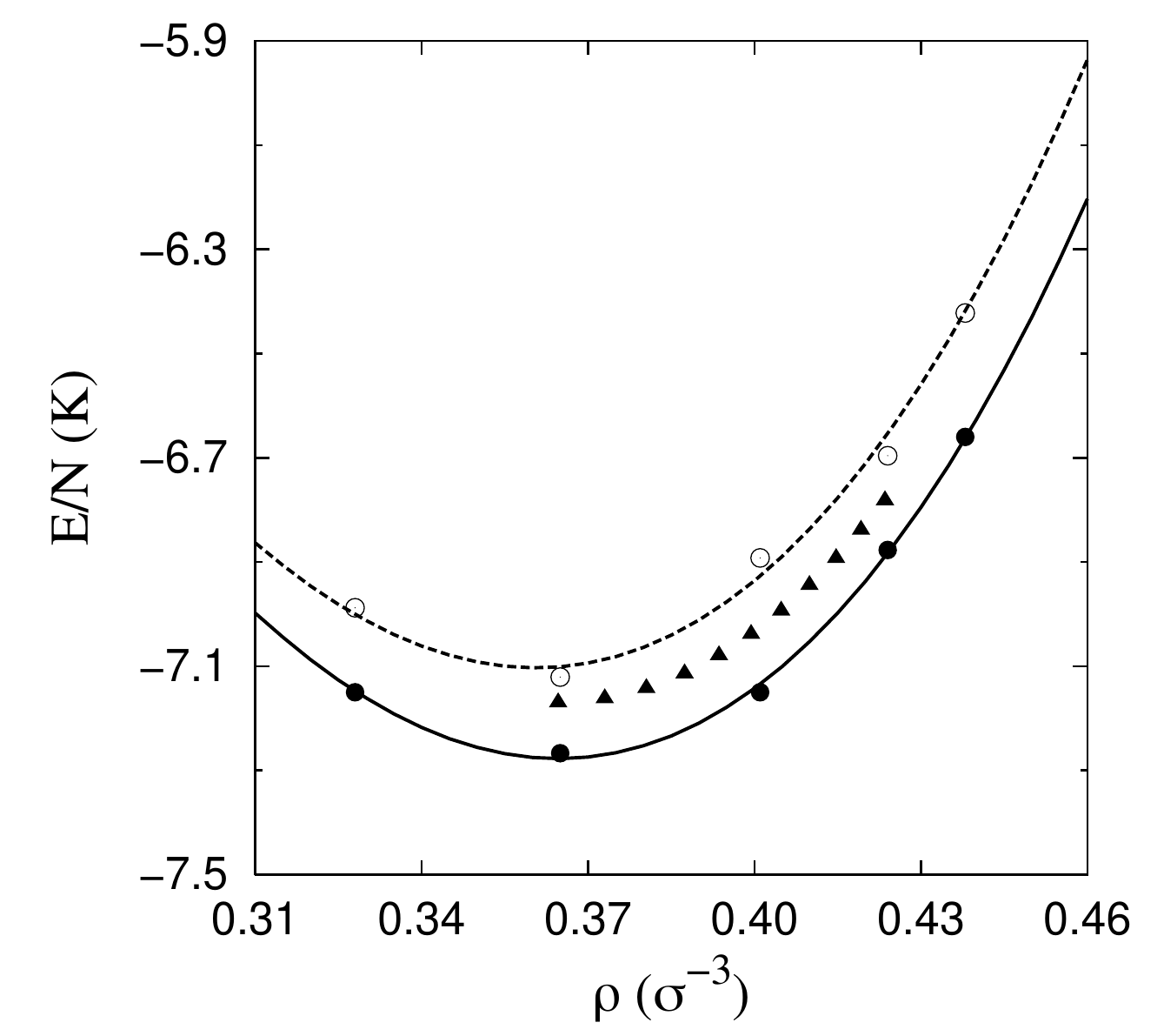
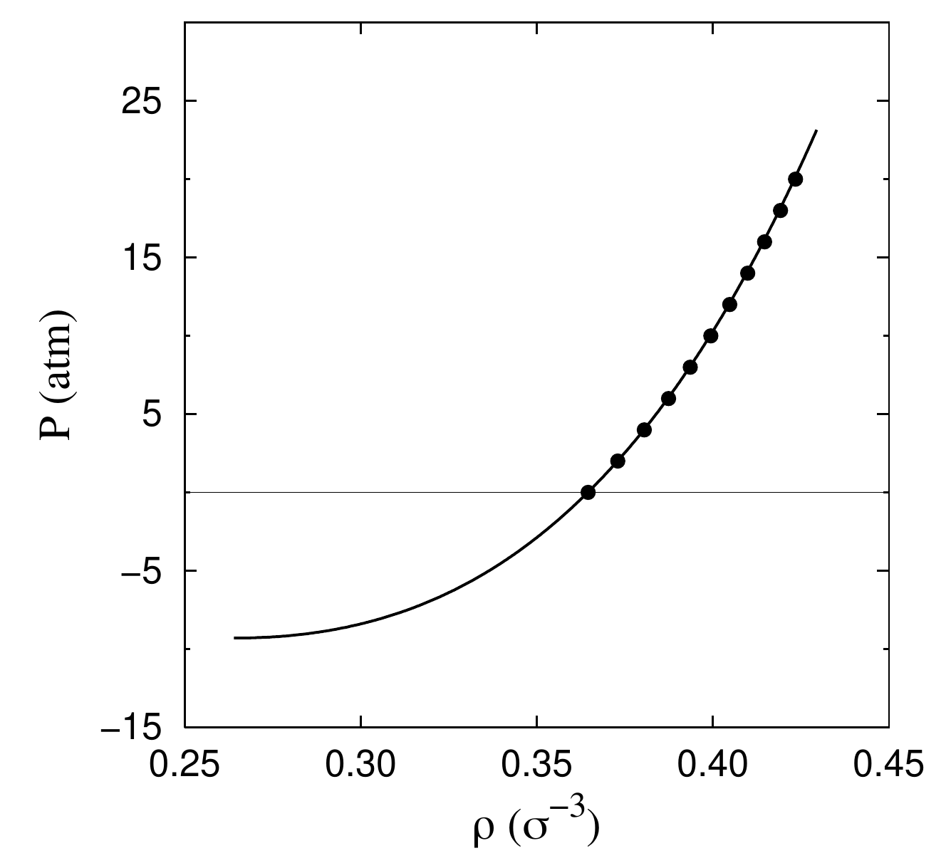
As it is shown in Fig. 2, the accuracy achieved by the DMC method to reproduce the experimental equation of state is impressive (Boronat and Casulleras, 1994). The dependence of the energy with the density is well reproduced, in spite of a nearly constant shift that it is related to the interatomic potential used in the simulations. We observe that the shift is practically constant looking at the dependence of the pressure with the density, as shown in Fig. 2.

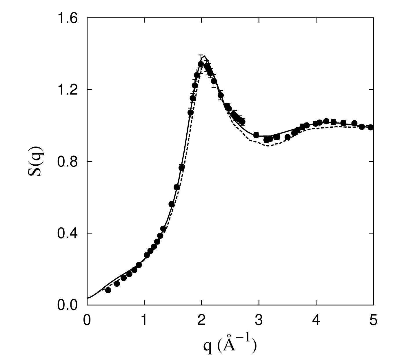
Quantum Monte Carlo methods are able to estimate other properties than the energy. However, direct estimations of operators which do not commute with the Hamiltonian are biased by the trial wave function used for importance sampling. To eliminate this bias it is necessary to work with pure estimators (Casulleras and Boronat, 1995), based on the forward-walking method (Liu, Kalos and Chester, 1974). In Fig. 3, we show DMC results for the static structure factor $S(q)$, calculated with pure estimators, in comparison with experimental data obtained from X-rays (Wirth and Hallock, 1987) and neutron scattering (Svensson et al., 1980). As one can see, the agreement between theory and experiment is excellent.

The study of the Fermi isotope ³He using Monte Carlo is much more involved due to the famous sign problem. In fact, the Monte Carlo interpretation of the imaginary-time Schrödinger equation requires that $f({\bf R},t)=\psi({\bf R})\Psi({\bf R},t)$ be a density, i.e., $\psi\,\Psi\geq 0$ in all the domain. This boundary condition can be satisfied if $\psi$ and $\Psi$ change sign together and thus share the same nodes. This approximation, known as fixed-node (FN) method, (Reynolds et al., 1982) has been extensively used in the ground-state calculations of Fermi quantum liquids. It can be proved that, due to that nodal constraint, the fixed-node energies are variational upper bounds to the exact eigenvalues for a given symmetry (Reynolds et al., 1982). Therefore, the FN results depend significantly on the quality of the trial wave function. The best upper bounds have been achieved by introducing backflow correlations, which move the nodal surface according to the interparticle interactions. Recently, an iterative backflow scheme has shown accurate results for the ³He equation of state (Taddei et al., 2015), in spite of being not so good as the ones obtained in ⁴He, where the calculation is not affected by the sign problem.

The thermal properties of liquid ⁴He have also been deeply studied using the path integral Monte Carlo (PIMC) method. As it is well known, the knowledge of the quantum partition function at finite temperature

$$Z=\text{Tr}\,e^{-\beta\hat{H}}$$

(41)

allows for a full microscopic description of the properties of a given system, with $\beta=1/T$ and $\hat{H}=\hat{K}+\hat{V}$ the Hamiltonian. The non-commutativity of the quantum operators, kinetic $\hat{K}$ and potential $\hat{V}$ energies, makes impractical a direct calculation of the partition function $Z$ (41). Instead, all practical implementations intended for Monte Carlo estimations of $Z$ rely on approximations that use as a starting point the convolution property

$$e^{-\beta(\hat{K}+\hat{V})}=\left(e^{-\varepsilon(\hat{K}+\hat{V})}\right)^{M}\ ,$$

(42)

with $\varepsilon=\beta/M$, where each one of the terms in the r.h.s. corresponds to a higher temperature $MT$. In the most simple approximation, known as primitive action (PA), the kinetic and potential contributions factorize

$$e^{-\varepsilon(\hat{K}+\hat{V})}\simeq e^{-\varepsilon\hat{K}}\,e^{-\varepsilon\hat{V}}\ ,$$

(43)

the convergence to the exact result being warranted by the Trotter formula (Trotter, 1959)

$$e^{-\beta(\hat{K}+\hat{V})}=\lim_{M\to\infty}\left(e^{-\varepsilon\hat{K}}\,e^{-\varepsilon\hat{V}}\right)^{M}\ .$$

(44)

The primitive action is a particular case of a more general expansion in which one can decompose the action, that is

$$e^{-\varepsilon(\hat{K}+\hat{V})}\simeq\prod_{i=1}^{n}e^{-t_{i}\varepsilon\hat{K}}\,e^{-v_{i}\varepsilon\hat{V}}\ ,$$

(45)

with $\{t_{i},v_{i}\}$ parameters to be determined. A particular implementation of this expansion put forward by Chin (Chin, 2004) has proved to be a full fourth-order approximation that even can behave as sixth order by tuning properly its free parameters (Sakkos, Casulleras and Boronat, 2009). Alternatively, one can use the pair-action approximation, in which the total action is built as product of pair actions that are obtained either exactly or with some approximations (Ceperley, 1995). Considering distinguishable particles, the quantum partition function $Z$ (41) can be obtained through a multidimensional integral of the $M$ terms (beads) in which it is decomposed,

$$Z=\int d\bm{R}_{1}\ldots d\bm{R}_{M}\ \prod_{\alpha=1}^{M}\rho(\bm{R}_{\alpha},\bm{R}_{\alpha+1})\ ,$$

(46)

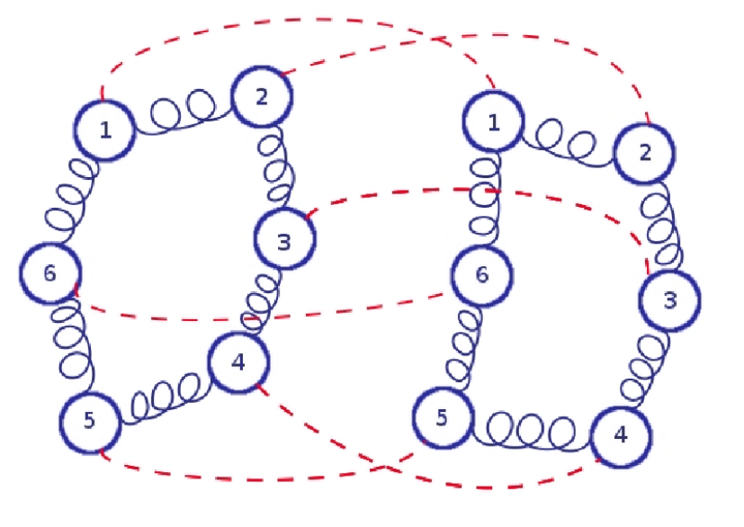
with $\bm{R}\equiv\{\bm{r}_{1},\ldots,\bm{r}_{N}\}$ and $\bm{R}_{M+1}=\bm{R}_{1}$. The PIMC method is then mapped to classical closed polymers composed by beads harmonically coupled by the kinetic action (Fig. 4).

To ensure the Bose symmetry of ⁴He it is necessary to symmetrize the quantum partition function (41). This requires of an additional sampling in the permutation space. The first applications of PIMC to liquid ⁴He were made by proposing permutations between pairs, triplets, and more particles (Ceperley, 1995). However, this method becomes inefficient when the total number of particles in the simulation increases. A significant better performance has been achieved with the introduction of the worm algorithm, first proposed in lattice systems (Prokof’ev, Svistunov and Tupitsyn, 1998), and then extended to continuum fluids (Boninsegni, Prokof’ev and Svistunov, 2006).

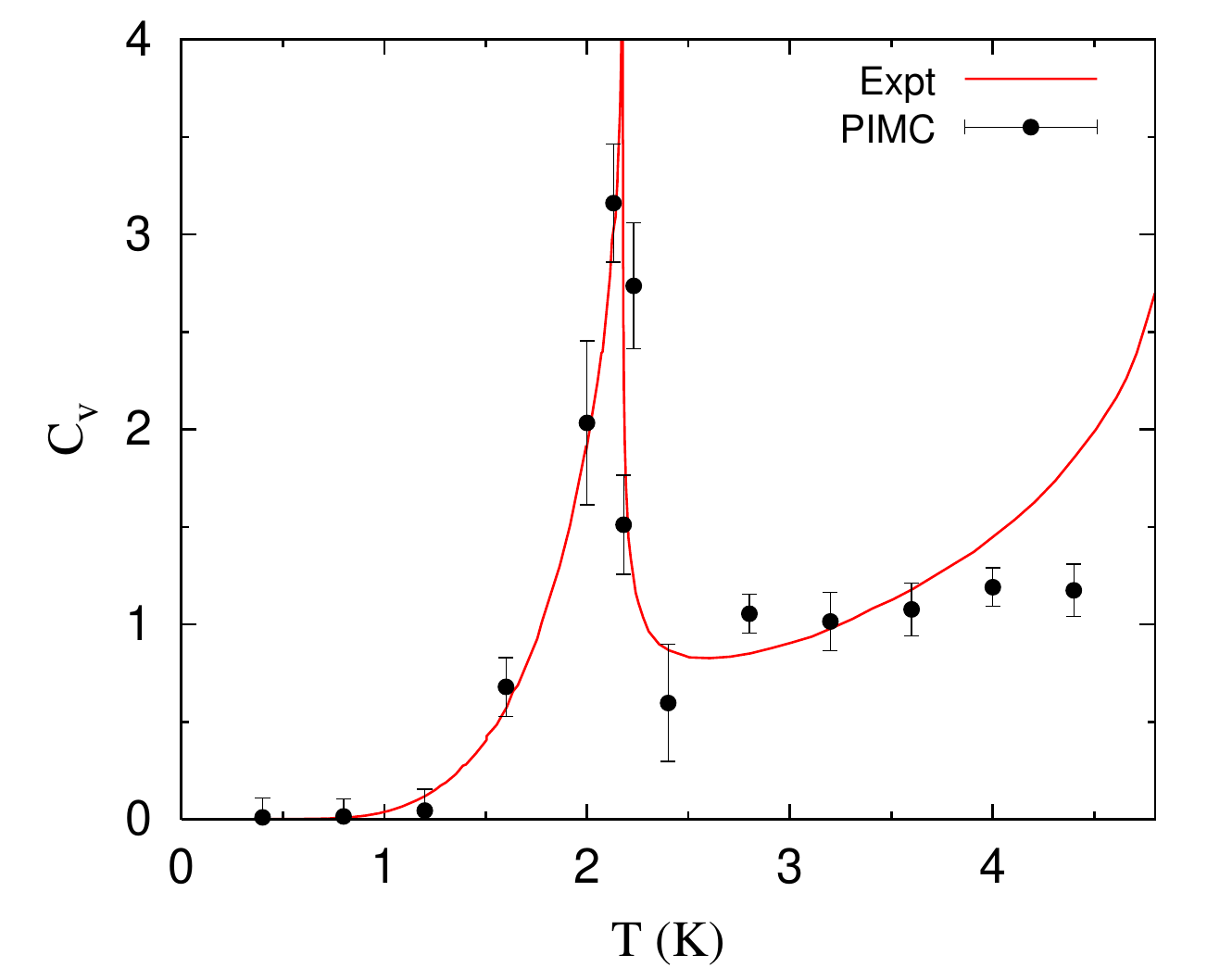
One of the more impressive successes of PIMC was the characterization of the normal-to-superfluid $\lambda$ phase transition at a critical temperature $T_{\lambda}=2.17$ K. In Fig. 5, we compare PIMC results of the specific heat as a function of $T$ with experimental data. The estimation of the specific heat is numerically involved but its singularity at $T_{\lambda}$ is well reproduced.

We have reported in this article some of the main theoretical approaches used in the study of liquid Helium. After an Introduction on the physical properties of liquid Helium, we have discussed the early theoretical approaches used in its study. In the third Section, we have discussed on the application of the variational theory and correlated basis function as a best approach for its microscopic understanding. In the fourth Section, we have introduced the main quantum Monte Carlo methods used in the study of liquid Helium.

This subject has been running for many years and it is impossible in practice to include all the immense work developed. Liquid Helium has been a continuous benchmark for quantum many-body theories and has been the workhorse for improving theories at all levels. This continued effort has produced a set of very accurate theoretical tools which have dramatically reproduced many experimental data. Liquid Helium is a really very strongly correlated quantum fluid where any simple perturbative scheme cannot be used. Remarkably, variational theory has proved to be the most efficient tool to deal with its microscopic description. Finally, it is also noticeable how progress in the development of quantum Monte Carlo methods has grown stimulated for the incredible amount of experimental data that we have at hands.

We acknowledge financial support from Ministerio de Ciencia e Innovación MCIN/AEI/10.13039/501100011033 (Spain) under Grant PID2020-113565GB-C21.

References

- (1)
- Allen and Misener (1938) Allen, J. F. and A. D. Misener. 1938. “Flow of liquid Helium II.” Nature 141:75.
- Arias de Saavedra et al. (1994) Arias de Saavedra, F., J. Boronat, A. Polls and A. Fabrocini. 1994. “Effective mass of one 4He atom in liquid 3He.” Phys. Rev. B 50:4248.
- Aziz, McCourt and Wong (1987) Aziz, R. A., F. R. W. McCourt and C. C. K. Wong. 1987. “A new determination of the ground state interatomic potential for He2.” Mol. Phys. 61:1487.
- Aziz et al. (1979) Aziz, R. A., V. P. S. Nain, J. S. Carley, W. L. Taylor and G. T. McConville. 1979. “An accurate intermolecular potential for Helium.” J. Chem. Phys. 70:4330.
- Balibar (2007) Balibar, S. 2007. “The discovery of superfluidity.” J. Low Temp. Phys. 146:441.
- Beauvois et al. (2018) Beauvois, K., J. Dawidowski, B. Fåk, H. Godfrin, E. Krotscheck, J. Ollivier and A. Sultan. 2018. “Microscopic dynamics of superfluid 4He: A comprehensive study by inelastic neutron scattering.” Phys. Rev. B 97:184520.
- Beliaev (1958) Beliaev, S. T. 1958. “Energy-spectrum of a non-ideal Bose gas.” Sov. Phys. JEPT 7:289.
- Bijl (1940) Bijl, A. 1940. Physica 7:869.
- Bogoliubov (1947) Bogoliubov, N. N. 1947. J. Phys. USSR 11:23.
- Boninsegni, Prokof’ev and Svistunov (2006) Boninsegni, M., N. V. Prokof’ev and B. V. Svistunov. 2006. “Worm algorithm and diagrammatic Monte Carlo: A new approach to continuous-space path integral Monte Carlo simulations.” Phys. Rev. E 74:036701.
- Boronat (2002) Boronat, J. 2002. Monte Carlo simulations at zero temperature: Helium in one, two, and three dimensions. In Microscopic Approaches to Quantum Liquids in Confined Geometries, ed. Eckhard Krotscheck and Jesús Navarro. Singapore: World Scientific pp. 21–90.
- Boronat, Fabrocini and Polls (1989) Boronat, J., A. Fabrocini and A. Polls. 1989. “Variational calculation of the binding energy of one 3He impurity in liquid 4He.” J. Low Temp. Phys. 74:347.
- Boronat, Polls and Fabrocini (1997) Boronat, J., A. Polls and A. Fabrocini. 1997. “Momentum distributions in 3He-4He mixtures.” Phys. Rev. B 56:11854.
- Boronat and Casulleras (1994) Boronat, J. and J. Casulleras. 1994. “Monte Carlo analysis of an interatomic potential for He.” Phy. Rev. B 49:8920.
- Campbell and Krotscheck (2009) Campbell, C. E. and E. Krotscheck. 2009. “Dynamic many-body theory: Pair fluctuations in bulk 4He.” Phys. Rev. B 80:174501.
- Campbell, Krotscheck and Lichtenegger (2015) Campbell, C. E., E. Krotscheck and T. Lichtenegger. 2015. “Dynamic many-body theory: Multiparticle fluctuations and the dynamic structure of 4He.” Phys. Rev. B 91:184510.
- Castillejo et al. (1979) Castillejo, L., A. D. Jackson, B. K. Jennings and R. A. Smith. 1979. “Optimal and nearly optimal distribution functions for 4He.” Phys. Rev. B 20:3631.
- Casulleras and Boronat (1995) Casulleras, J. and J. Boronat. 1995. “Unbiased estimators in quantum Monte Carlo methods: Application to liquid 4He.” Phys. Rev. B 52:3654.
- Ceperley (1995) Ceperley, D. M. 1995. “Path integrals in the theory of condensed Helium.” Rev. Mod. Phys. 67:279.
- Chakraborty (1982) Chakraborty, Tapash. 1982. “Variational theory of binary boson mixture at K.” Phys. Rev. B 25:3177.
- Chin (2004) Chin, S. A. 2004. “Quantum statistical calculations and symplectic corrector algorithms.” Phys. Rev. E 69:046118.
- Clements et al. (1993) Clements, B. E., J. L. Epstein, E. Krotscheck and M. Saarela. 1993. “Structure of boson quantum films.” Phys. Rev. B 48:7450.
- De Bruyn Ouboter and Yang (1987) De Bruyn Ouboter, R. and C. N. Yang. 1987. “The thermodynamic properties of liquid 3He-4He mixtures between 0 and 20 atm in hte limit of absolute zero temperature.” Physica B 44:127.
- Ebner and Edwards (1970) Ebner, C. and D. O. Edwards. 1970. “The low temperature thermodynamic properties of superfluid solutions of 3He in 4He.” Phys. Rep. 2:77.
- Fabrocini and Polls (1982) Fabrocini, A. and A. Polls. 1982. “Variational study of 3He-4He mixture.” Phys. Rev. B 25:4533.
- Fabrocini and Rosati (1982) Fabrocini, A. and S. Rosati. 1982. “The method of interpolating integral equations for quantum fluids.—II.” Nuovo Cimento D 1:615.
- Fabrocini and Rosati (1988) Fabrocini, A. and S. Rosati. 1988. Correlated basis function theory for fermion systems. In First International Course on Condensed Matter. Singapore: Ed. D. Prosperi et al.,World Scientific pp. 89–150.
- Fantoni (1978) Fantoni, S. 1978. Nuovo Cimento A 44:191.
- Fantoni and Rosati (1975) Fantoni, S. and S. Rosati. 1975. “The hypernetted-chain approximation for a fermion system.” Nuovo Cimento A 25:593.
- Feenberg (1969) Feenberg, E. 1969. Theory of Quantum Fluids. Academic Press, New York.
- Feynman (1953) Feynman, R. P. 1953. “Atomic theory of the transition in Helium.” Phys. Rev. 91:1291.
- Feynman and Cohen (1956) Feynman, R. P. and M. Cohen. 1956. “Energy spectrum of the excitations in liquid Helium.” Phys. Rev. 102:1189.
- Glyde (1994) Glyde, Henry R. 1994. Excitations in liquid and solid Helium. Clarendon Press, Oxford.
- Godfrin et al. (2012) Godfrin, H., M. Meschke, H. J. Lauter, A. Sultan, H. Böhm, E. Krotscheck and M. Panholzer. 2012. “Observation of a roton collective mode in a two-dimensional Fermi liquid.” Nature 483:576.
- Hugenholtz and Pines (1959) Hugenholtz, N. and D. Pines. 1959. “Ground-State energy and excitation spectrum of a system of interacting bosons.” Phys. Rev. 116:489.
- Jackson, Lande and Lantto (1979) Jackson, A. D., A. Lande and L. J. Lantto. 1979. “Euler-Lagrange equations and hypernetted chain calculations of boson matter.” Nucl. Phys. A 317:70.
- Jackson and Feenberg (1962) Jackson, H. W. and E. Feenberg. 1962. “Energy Spectrum of Elementary Excitations in Helium II.” Rev. Mod. Phys. 34:686.
- Jastrow (1955) Jastrow, R. 1955. “Many-Body problem with strong forces.” Phy. Rev. 98:1479.
- Kallio and Smith (1977) Kallio, A. and R. A. Smith. 1977. “How simple can HNC be – and still be right?” Phys. Lett. B 68:315.
- Kamerlingh Onnes (1908) Kamerlingh Onnes, H. 1908. Proc. Sect. Sci. K. ned. Akad. Wet. 11:168.
- Kapitza (1938) Kapitza, P. 1938. “Viscosity of liquid Helium below the lambda point.” Nature 141:74.
- Keesom and Clusius (1932) Keesom, W. H. and K. Clusius. 1932. Proc. Sect. Sci. K. ned. Akad. Wet. 35:307.
- Krotscheck (2000) Krotscheck, E. 2000. “Fermi-Hypernetted chain theory for liquid 3He: a reassessment.” J. Low Temp. Phys. 119:103.
- Krotscheck and Ristig (1975) Krotscheck, E. and M. L. Ristig. 1975. “Long-range Jastrow correlations.” Nucl. Phys. A 242:389.
- Landau (1941) Landau, L. D. 1941. “Theory of the superfluidity of Helium II.” Phys. Rev. 60:356.
- Landau (1947) Landau, L. D. 1947. J. Phys. USSR 11:91.
- Lantto, Jackson and Siemens (1977) Lantto, L. J., A. D. Jackson and P. J. Siemens. 1977. “HNC variational calculations of boson matter.” Phys. Lett. B 68:311.
- Lee and Lee (1975) Lee, D. K. and F. J. Lee. 1975. “Brillouin-Wigner perturbation procedure for elementary excitations in liquid 4He.” Phys. Rev. B 11:4318.
- Lee, Huang and Yang (1957) Lee, T. D., K. Huang and C. N. Yang. 1957. “Eigenvalues and eigenfunctions of a Bose system of hard spheres and its low-temperature properties.” Phys. Rev. 106:1135.
- Liu, Kalos and Chester (1974) Liu, K. S., M. H. Kalos and G. V. Chester. 1974. “Quantum hard spheres in a channel.” Phys. Rev. A 10:303.
- London (1938) London, F. 1938. “The -Phenomenon of Liquid Helium and the Bose-Einstein Degeneracy.” Nature 141:643.
- Manousakis et al. (1983) Manousakis, E., S. Fantoni, V.R. Pandharipande and Q.N. Usmani. 1983. “Microscopic calculations for normal and polarized liquid 3He.” Phys. Rev. B 28:3770.
- Pandharipande (1978) Pandharipande, V. R. 1978. “Three-body correlations in the variational wave function of liquid 4He.” Phys. Rev. B 18:218.
- Pitaevskii and Stringari (2016) Pitaevskii, L. and S. Stringari. 2016. Bose-Einstein Condensation and Superfluidity. Oxford University Press, Oxford.
- Prokof’ev, Svistunov and Tupitsyn (1998) Prokof’ev, N. V., B. V. Svistunov and I. S. Tupitsyn. 1998. “Worm algorithm in quantum Monte Carlo simulations.” Phys. Lett. A 238:253.
- Reynolds et al. (1982) Reynolds, P. J., D. M. Ceperley, B. J. Alder and W. A. Lester Jr. 1982. “Fixed node quantum Monte Carlo for molecules.” J. Chem. Phys. 77:5593.
- Rosati (1981) Rosati, S. 1981. FHNC variational theory for strongly interacting Fermi systems. In From Nuclei to Particles, Proceedings of the International School of Physics Enrico Fermi, Course LXXIX. Amsterdam: Ed. A. Molinari, North Holland pp. 73–112.
- Sakkos, Casulleras and Boronat (2009) Sakkos, K., J. Casulleras and J. Boronat. 2009. “High order Chin actions in path integral Monte Carlo.” J. Chem. Phys. 130:204109.
- Svensson et al. (1980) Svensson, E. C., V. F. Sears, A. D. B. Woods and P. Martel. 1980. “Neutron-diffraction study of the static structure factor and pair correlations in liquid 4He.” Phys. Rev. B 21:3638.
- Taddei et al. (2015) Taddei, M., M. Ruggeri, S. Moroni and M. Holzmann. 2015. “Iterative backflow renormalization procedure for many-body ground-state wave functions of strongly interacting normal Fermi liquids.” Phys. Rev. B 91:115106.
- Tisza (1938) Tisza, L. 1938. “Transport phenomena in Helium II.” Nature 141:913.
- Trotter (1959) Trotter, H. F. 1959. “On the product of semi-groups of operators.” Proc. Am. Math. Soc. 10:545.
- Usmani, Friedman and Pandharipande (1982) Usmani, Q. N., B. Friedman and V. R. Pandharipande. 1982. “Scaling approximation for the elementary diagrams in hypernetted-chain calculations.” Phy. Rev. B 25:4502.
- Usmani, Fantoni and Pandharipande (1982) Usmani, Q. N., S. Fantoni and V. R. Pandharipande. 1982. “Three-body correlations in liquid 4He.” Phys. Rev. B 26:6123.
- Wilks (1967) Wilks, J. 1967. Liquid and solid Helium. Clarendon Press, Oxford.
- Wirth and Hallock (1987) Wirth, F. H. and R. B. Hallock. 1987. “X-ray determinations of the liquid-structure factor and pair-correlation function of 4He.” Phys. Rev. B 35:89.
- Wu (1959) Wu, T. T. 1959. “Ground state of a Bose system of hard spheres.” Phys. Rev. 115:1390.