Theory and Techniques for Synthesizing a Family of Graph Algorithms

The basic steps in guided program synthesis are:

1. 1.

   Start with a logical specification of the problem to be solved. A specification is a quadruple $\langle D,R,o,c\rangle$ where $D$ is an input type, $R$ an output or result type, $o:D\times R$ is a predicate relating correct or feasible outputs to inputs, and $c:D\times R\rightarrow Int$ is a cost function on solutions. An example specification is in Eg. 1 (This specification is explained in more detail below)

2. 2.

   Pick an algorithm class from a library of algorithm classes (Global Search, Local Search, Divide and Conquer, Fixpoint Iteration, etc). An algorithm class comprises a program schema containing operators to be instantiated and an axiomatic theory of those operators (see [10] for details). A schema is analogous to a template in Java/C++ , with the difference that both the template and template arguments are formally constrained.

3. 3.

   Instantiate the operators of the program schema using information about the problem domain and in accordance with the axioms of the class theory. To ensure correctness, this step can be carried out with mechanical assistance. The result is an efficient algorithm for solving the given problem.

4. 4.

   Apply low-level program transforms such as finite differencing, context-dependent simplification, and partial evaluation, followed by code generation. Many of these are automatically applied by Specware [2], a formal program development environment.

The result of Step 4 is an efficient program for solving the problem which is guaranteed correct by construction. The power of the approach stems from the fact that the common structure of many algorithms is contained in one reusable program schema and associated theory. Of course the program schema needs to be carefully designed, but that is done once by the library designer. The focus of this paper is the Global Search class, and specifically on how to methodically carry out Step 3 for a wide variety of problems. Details of the other algorithm classes and steps are available elsewhere [8, 16, 14].

Before delving into a program schema for Global Search, it helps to understand the structures over which the program schema operates. In [16], a search space is represented by a descriptor of some type $\widehat{R}$, which is an abstraction of the result type $R$. The initial or starting space is denoted $\bot$. There are also two predicates split$:D\times\widehat{R}\times\widehat{R}$, written $\pitchfork$, and extract$:\widehat{R}\times R$, written $\chi$. Split defines when a space is a subspace of another space, and extract captures when a solution is extractable from a space. We say a solution $z$ is contained in a space $y$ (written $z\in y$) if it can be extracted after a finite number of splits. A feasible space is one that contains feasible solutions. We often write $\pitchfork(x,y,y^{\prime})$ as $y\pitchfork_{x}y^{\prime}$ for readability, and even drop the subscript when there is no confusion. Global Search theory (GS-theory) [16] axiomatically characterizes the relation between the predicates $\bot$, $\pitchfork$ and $\chi$, as well as ensuring that the associated program schema computes a result that satisfies the specification. In the sequel, the symbols $\widehat{R},\bot,\pitchfork,\chi,\oplus$ are all assumed to be drawn from GS-theory. A theory for a given problem is created by instantiating these terms, as shown in the next example.

As mentioned in the introduction, a dominance relation provides a way of comparing two subspaces in order to show that one will always contain at least as good a solution as the other. (Goodness in this case is measured by some cost function on solutions). The first space is said to dominate ($\vartriangleright$) the second, which can then be eliminated from the search. Letting $c^{*}$ denote the cost of an optimal solution in a space, this can be formalized as (all free variables are assumed to be universally quantified):

$$y\vartriangleright y^{\prime}\Rightarrow c^{*}(x,y)\leq c^{*}(x,y^{\prime})$$

(2.1)

Another way of expressing the consequent of (2.1) is

$$\forall z^{\prime}\in y^{\prime}\cdot\,o(x,z^{\prime})\Rightarrow\exists z\in y\cdot\,o(x,z)\wedge c(x,z)\leq c(x,z^{\prime})$$

(2.2)

To derive dominance relations, it is often useful to first derive a semi-congruence relation [16]. A semi-congruence between two partial solutions $y$ and $y^{\prime}$, written $y\rightsquigarrow y^{\prime}$, ensures that any way of extending $y^{\prime}$ into a feasible solution can also be used to extend $y$ into a feasible solution. Like $\pitchfork$, $\rightsquigarrow$ is a ternary relation over $D\times\widehat{R}\times\widehat{R}$ but as we have done with $\pitchfork$ and many other such relations in this work, we drop the input argument when there is no confusion and write it as a binary relation for readability. Before defining semi-congruence, we introduce two concepts. One is the idea of useability of a space. A space $y$ is is useable, written $o^{*}(x,y)$, if $\exists z.\,\chi(y,z)\wedge o(x,z)$, meaning a feasible solution can be extracted from the space. The second is the notion of incorporating sufficient information into a space to make it useable. This is defined by an operator $\oplus:\widehat{R}\times t\rightarrow\widehat{R}$ that takes a space and some additional information of type $t$ and returns a more defined space. The type $t$ depends on $\widehat{R}$. For example if $\widehat{R}$ is the type of lists, then $t$ might also be the same type. Now the formal definition of semi-congruence is:

$$y\rightsquigarrow y^{\prime}\Rightarrow o^{*}(x,y^{\prime}\oplus e)\Rightarrow o^{*}(x,y\oplus e)$$

That is, $y\rightsquigarrow y^{\prime}$ is a sufficient condition for ensuring that if $y^{\prime}$ can be extended into a feasible solution than so can $y$ with the same extension. If $c$ is compositional (that is, $c(s\oplus t)=c(s)+c(t)$) then it can be shown [10] that if $y\rightsquigarrow y^{\prime}$ and $y$ is cheaper than $y^{\prime},$ then $y$ dominates $y^{\prime}$ (written $y\vartriangleright y^{\prime}$). Formally:

$$y\rightsquigarrow y^{\prime}\wedge c(x,y)\leq c(x,y^{\prime})\Rightarrow y\vartriangleright y^{\prime}$$

(2.3)

The axioms given above extend GS-theory [16].

The remaining sections cover the original contributions of this paper.

A program theory for EBFS defines a recursive function which given a space $y$, computes a non-trivial subset $F_{x}(y)$ of the optimal solutions contained in $y$, where

$$F_{x}(y)=opt_{c}\{z\mid z\in y\wedge o(x,z)\}$$

$opt_{c}$ is a subset of its argument that is the optimal set of solutions (w.r.t. the cost function $c$), defined as follows:

$$opt_{c}S=\{z\mid z\in S\wedge(\forall z^{\prime}\in S\,\cdot\,c(z)\leq c(z^{\prime}))\}$$

Also let $undom(y)$ be $undom_{l(y)+1}\cap\{yy\mid y\pitchfork yy\}$ where $l(y)$ is the level of $y$ in the tree. The following proposition defines a recurrence for computing the feasible solutions in a space:

Finally he following theorem defines a recurrence that can be used to compute $FO_{x}(y)$:

The theorem states that if the feasible solutions immediately extractable from a space $y$ are combined with the solutions obtained from $GO_{x}$ of each undominated subspace $yy$, and the optimal ones of those retained, the result is a subset of $FO_{x}(y)$. The next theorem demonstrate non-triviality³³3Non-triviality is similar but not identical to completeness. Completeness requires that every optimal solution is found by the recurrence, which we do not guarantee. of the recurrence by showing that if a feasible solution exists in a space, then one will be found.

From the characteristic recurrence we can straightforwardly derive a simple recursive function bfs to compute a non-trivial subset of $F_{x}$ for a given $y$, shown in Alg. 1

The final program schema that is included in the Specware library is the result of incorporating a number of other features of GS such as necessary filters, bounds tests, and propagation, which are not shown here. Details of these and other techniques are in [16].

A greedy algorithm [3] is one which repeatedly makes a locally optimal choice. For some classes of problems this leads to a globally optimum choice. We can get a characterization of optimally greedy algorithms within EBFS by restricting the size of $undom_{l}$ for any $l$ to 1. If $undom_{l}\neq\emptyset$ then the singleton member $y^{*}$ of $undom_{l}$ is called the greedy choice. In other work [13] we show how to derive greedy algorithms for a variety of problems including Activity Selection, One machine scheduling, Professor Midas’ Traveling Problem, Binary Search.

Previously in Eg. 8 we derived a dominance relation for the (undirected) single pair shortest path problem. To solve the problem of finding all shortest paths from a given start node to every other node in the graph it is convenient to consider the output as a set of edges that form what is called a path tree, a subgraph of the input graph which forms a spanning tree rooted at the start node. The desired output is a path tree in which every path from the root is the shortest. The specification of Single Pair Shortest Path in Fig. 2.1 is revised as shown in Fig. 5.1

The revised instantiation of Global Search theory is shown in Fig. 5.2

In what follows, the extends operator $\oplus$ is shown by simple concatenation. The goal is to show that there is at most one undominated child following a split of a partial solution $\alpha$. Let $\alpha e$ and $\alpha e^{\prime}$ be two children following a split of $\alpha$, that is the graphs $\alpha$ with edge $e$ added and that with $e^{\prime}$ added. Without loss of generality (w.l.o.g.) assume neither $e$ nor $e^{\prime}$ are already contained in $\alpha$ and both connect to $\alpha$. Let $z^{\prime}=\alpha e^{\prime}\omega^{\prime}$ be a feasible solution derived from $\alpha e^{\prime}$. The task is to construct a feasible solution $z$ from $\alpha e$ and discover the conditions under which it is cheaper than $z^{\prime}$. We will use the definition of general dominance (2.2), repeated here for convenience:

$$\forall z^{\prime}\in y^{\prime}\cdot\,o(x,z^{\prime})\Rightarrow\exists z\in y\cdot\,o(x,z)\wedge c(x,z)\leq c(x,z^{\prime})$$

Establishing $o(\alpha e\omega)$ requires connected$(\alpha e\omega)$ and acyclic$(\alpha e\omega)$.

In guided program synthesis, it is often useful to write down laws [17] that will be needed during the derivation. Some of the most useful laws are distributive laws and monotonicity laws. For example the following distributive law applies to $ayclic$ :

$$\mathit{acyclic}(\alpha\beta)=\mathit{acyclic}(\alpha)\wedge\mathit{acyclic}(\beta)\wedge\mathit{ac}(\alpha,\beta)$$

where $ac$ defines what happens at the “boundary” of $\alpha$ and $\beta$:

$$\mathit{ac}(\alpha,\beta)=\forall m,n\cdot\,\exists p\in\alpha^{*}\cdot\,path?(p,m,n)\Rightarrow\neg\exists q\in\beta^{*}\cdot\,path?(q,m,n)$$

requiring that if $p$ is a path in $\alpha$ ($\alpha^{*}$ is a regular expression denoting all possible sequences of edges in $\alpha$) connecting $m$ and $n$ then there should be no path between $m$ and $n$ in $\beta$. Examples of monotonicity laws are $acyclic(\alpha\beta)\Rightarrow acyclic(\alpha)$ and $connected(\alpha)\wedge connected(\beta)\wedge nodes(\alpha)\cap nodes(\beta)\neq\emptyset\Rightarrow connected(\alpha\beta$). By using the laws constructively, automated tools such as KIDS [17] can often suggest instantiations for terms. For instance, after being told $connected(\alpha e^{\prime}\omega^{\prime})$, the tool could apply the monotonicity law for $connected$ to suggest $connected(\alpha ee^{\prime}\omega^{\prime})$, that is to try $\omega=e^{\prime}\omega^{\prime}$. With this binding for $\omega$ we can attempt to establish $acyclic(\alpha e\omega)$, by expanding its definition. One of the terms is $\ldots ac($$e,\alpha e^{\prime}\omega^{\prime})\ldots$ which fails because $conn(\alpha e^{\prime}\omega^{\prime})$ implies $path?(\alpha e^{\prime}\omega^{\prime},e.a,e.b)$ so adding edge $e$ creates a cycle. The witness to the failure is some path $\pi^{\prime}=e_{j}\ldots e_{k}$ where $e_{j}.a=e.a\wedge e_{k}.b=e.b$. One possibility is that $e_{j}=e_{k}=e$, that is $\omega^{\prime}$ contains $e$. If so, let $\omega^{\prime}=e\psi^{\prime}$ for some $\psi^{\prime}$. Then $z^{\prime}=\alpha e^{\prime}\omega^{\prime}=\alpha e^{\prime}e\psi^{\prime}=\alpha ee^{\prime}\psi^{\prime}$. Let $\omega=e^{\prime}\psi^{\prime}$ and now $z=z^{\prime}$. Otherwise, w.l.o.g assume that $e$ connects with $\alpha$ at $e.a$, and therefore so does $e_{j}$, so the case $e_{j}.b=e.b$ is not very interesting. The only option then is to remove edge $e_{k}$ from $\omega^{\prime}$ . Let $\omega^{\prime}=e_{k}\psi^{\prime}$ and so $\omega$ is $e^{\prime}\psi^{\prime}$. Now the requirement becomes

$$acyclic(\alpha e)\wedge acyclic(e^{\prime}\psi^{\prime})\wedge ac(\alpha e,e^{\prime}\psi^{\prime})$$

$acyclic(e^{\prime}\psi^{\prime})$ follows from $acyclic(\alpha e^{\prime}\psi^{\prime})$ by monotonicity and $ac(\alpha e,e^{\prime}\psi^{\prime})$ follows from $acyclic(\alpha e^{\prime}\psi^{\prime})$ and the fact that $e$ was chosen above to remove the cycle in $\alpha ee^{\prime}\omega^{\prime}$ . This demonstrates $o(\alpha e\omega)$ provided $acyclic(\alpha e)$ where $\omega$ is constructed as above.

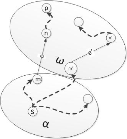
Finally, to establish general dominance it is necessary to show that $z$ costs no more than $z^{\prime}$. Note that the cost of a solution is the sum of individual path costs starting from $x.s$. Let $m$ denote $e.a$ and $n$ denote $e.b$ (and analogously for $e^{\prime}$). Now consider a path to a node $p$ in $z^{\prime}$. If the path to $p$ does not contain edge $e_{k}$ ie. pass through $n$ then the same path holds in $z$. Otherwise let $\beta^{\prime}e^{\prime}_{i}\gamma^{\prime}e"\delta$ be a path to $p$ in $z^{\prime}$ where $e"$ is the edge $e_{k}$ above (see Fig. 5.3).

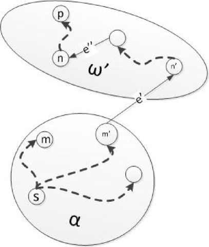
$\beta^{\prime}$ is a path from $x.s$ in $\alpha$ and $e^{\prime}_{i}$ is some edge that leads out of $\alpha$ on the path to $p$. Then the corresponding path in $z$ is $\beta e\delta$ (see Fig. 5.4).

$$\begin{array}[]{l}c(\alpha e\omega,\beta e\delta)\leq c(\alpha e^{\prime}\omega^{\prime},\beta^{\prime}e{}_{i}\gamma^{\prime}e"\delta)\\ =\{\mbox{expand defns}\}\\ c(z,\beta e)+c(z,\delta)\leq c(z^{\prime},\beta^{\prime}e_{i})+c(z^{\prime},e")+c(z,\delta)\\ =\{\mbox{+ve edge weights, triangle inequality}\}\\ c(z,\beta e)\leq c(z^{\prime},\beta^{\prime}e{}_{i})\end{array}$$

As there were no restrictions on $e^{\prime}$ above, let $e_{i}$ be the witness for $e^{\prime}$ and this establishes

That is, provided the path $\beta e$ is shorter than $\beta^{\prime}e^{\prime}$, there cannot be a shorter path via $e^{\prime}$ to $n$. As cost is the sum of the path costs, it follows that $c(x,\alpha e\omega)\leq c(\alpha e^{\prime}\omega^{\prime})$. The dominance condition is then $\alpha e\vartriangleright\alpha e^{\prime}\Leftarrow acyclic(\alpha e)\wedge c(z,\beta e)\leq c(z^{\prime},\beta^{\prime}e^{\prime})$ . Finally, as it is not known at the time of the split which $e^{\prime}$ will lie on the path to $e.b$, to be conservative, let $e$ be that edge whose endpoint $e.b$ is the closest to the start node. This is therefore the greedy choice. Iincorporating finite differencing to incrementally maintain the distances to the nodes, using the dominance relation derived earlier for Single Pair Shortest Path to eliminate the longer paths to a node, and data structure refinement results in an algorithm similar to Dijkstra’s algorithm for MSTs.

The specification of MST is very similar to that of Shortest Path, with the difference that there is no longer a distinguished node $s$, the input graph must be connected, and the cost of a solution is simply the sum of the weights of the edges in the tree

The instantiation of the simple GS operators is as for SP. Again, any edge that is added must not create a cycle or it cannot lead to a feasible solution. We will describe the algorithm construction process informally so as to expose the connection with the Shortest Path algorithm more clearly. However the derivations shown here can also be similarly formalized.

There are now two ways to satisfy the acyclicity requirement. One is by choosing an edge connecting a node in $\alpha$ to one outside of $\alpha$. Another is to choose an edge that connects two nodes within $\alpha$, being careful not to create cycles. The two options are examined next,

Option 1: Let $z^{\prime}=\alpha e^{\prime}\omega^{\prime}$ be a feasible solution derived from $\alpha e^{\prime}$. If $\omega^{\prime}$ includes $e$ then let $\omega$ in a feasible solution $z=\alpha e\omega$ simply be $\omega^{\prime}-\{e\}\cup\{e^{\prime}\}$ and then $z=z^{\prime}$. Otherwise, if $\omega$’ does not contain $e$ there must be some other path connecting $\alpha$ with $e.t$. W.l.o.g. assume that path is via $e^{\prime}$. If $\alpha e^{\prime}\omega^{\prime}$ is feasible, then it is a tree, so $\omega$’ is also a tree. Therefore it is not difficult to show that $z=\alpha e\omega^{\prime}$ is also a spanning tree. Now to show dominance, derive conditions under which $z$ is cheaper than $z^{\prime}$:

$$\begin{array}[]{l}c(x,\alpha e\omega^{\prime})\leq c(x,\alpha e^{\prime}\omega^{\prime})\\ =\{\mbox{defn of }c\}\\ \sum_{edge\in\alpha e\omega^{\prime}}edge.w\leq\sum_{edge\in\alpha e^{\prime}\omega^{\prime}}edge.w\\ =\\ e.w\leq e^{\prime}.w\end{array}$$

Finally, as it is not known at the time of the split which $e^{\prime}$ will lie on the path to $e.t$, to be conservative, let $e$ be that edge with the least weight connecting $\alpha$ with an external node . This is therefore the greedy choice. The result is an algorithm that is similar to Prim’s algorithm for MSTs.

Option 2: The difference with Option 1 is in how $e$ is chosen in order to ensure acyclicity. For a feasible solution, $\alpha$ must not contain any cycles. Therefore it consists of a collection of acyclic connected components, ie trees. Any new edge cannot connect nodes within a component without introducing a cycle. Therefore it must connect two component trees. Connecting two trees by a single edge results in a new tree. As in Option 1, let $z^{\prime}=\alpha e^{\prime}\omega^{\prime}$ be a feasible solution derived from $\alpha e^{\prime}$. If $\omega^{\prime}$ includes $e$ then let $\omega$ in a feasible solution $z=\alpha e\omega$ simply be $\omega^{\prime}-\{e\}\cup\{e^{\prime}\}$ and then $z=z^{\prime}$. Otherwise, if $\omega$’ does not contain $e$ there must be some other edge used to connect the two trees that $e$ would have connected. W.l.o.g. assume that edge is $e^{\prime}$. If $\alpha e^{\prime}\omega^{\prime}$ is feasible, then it is a tree, so $\omega$’ is also a tree. Therefore it is not difficult to show that $z=\alpha e\omega^{\prime}$ is also a spanning tree. The derivation of a cost comparison relation is identical to Option 1, and once again the greedy choice is the edge $e$ that connects two trees and is of least weight. The result of this option is an algorithm that is similar to Kruskal’s algorithm.

In conclusion, we observe that far from being completely different algorithms, Dijkstra’s algorithm, Prim’s algorithm and Kruskal’s algorithm differ only in very small number of (albeit important) ways. In contrast, many textbook descriptions of the algorithms introduce the algorithms out of the blue, followed by separate proofs of correctness. We have shown how a systematic procedure can derive different algorithms, with relatively minor changes to the derivations.

References

- [1]
- [2] Specware. Http://www.specware.org.
- [3] T. Cormen, C. Leiserson, R. Rivest & C. Stein (2001): Introduction to Algorithms, 2nd edition. MIT Press.
- [4] R Dechter (2003): Constraint Processing. Morgan Kauffman.
- [5] S. Gulwani, S. Jha, A. Tiwari & R. Venkatesan (2011): Synthesis of loop-free programs. In: PLDI, pp. 62–73, 10.1145/2F1993498.1993506.
- [6] T. Ibaraki (1977): The Power of Dominance Relations in Branch-and-Bound Algorithms. J. ACM 24(2), pp. 264–279, 10.1145/2F322003.322010.
- [7] S. Itzhaky, S. Gulwani, N. Immerman & M. Sagiv (2010): A simple inductive synthesis methodology and its applications. In: OOPSLA, pp. 36–46, 10.1145/2F1869459.1869463.
- [8] C. Kreitz (1998): Program Synthesis. In W. Bibel & P. Schmitt, editors: Automated Deduction – A Basis for Applications, chapter III.2.5, III, Kluwer, pp. 105–134.
- [9] K. R. M. Leino (2010): Dafny: an automatic program verifier for functional correctness. In: Proc. 16th intl. conf. on Logic for Prog., AI, & Reasoning, LPAR, pp. 348–370, 10.1007/2F978-3-642-17511-4_20.
- [10] S. Nedunuri (2012): Theory and Techniques for Synthesizing Efficient Breadth-First Search Algorithms. Ph.D. thesis, Univ. of Texas at Austin.
- [11] S. Nedunuri & W.R. Cook (2009): Synthesis of Fast Programs for Maximum Segment Sum Problems. In: Intl. Conf. on Generative Prog. and Component Engineering (GPCE), 10.1145/2F1621607.1621626.
- [12] S. Nedunuri, D. R. Smith & W. R. Cook (2010): A Class of Greedy Algorithms and Its Relation to Greedoids. Intl. Colloq. on Theoretical Aspects of Computing (ICTAC), 10.1007/2F978-3-642-14808-8_24.
- [13] S. Nedunuri, D. R. Smith & W. R. Cook (2012): Theory and Techniques for a Class of Efficient Breadth-First Search Algorithms. In: Intl. Symp. on Formal Methods (FM).
- [14] D. Pavlovic, P. Pepper & D. R. Smith (2010): Formal Derivation of Concurrent Garbage Collectors. In: Math. of Program Constr. (MPC), 10.1007/2F978-3-642-13321-3_20.
- [15] Y. Pu, R. Bodík & S. Srivastava (2011): Synthesis of first-order dynamic programming algorithms. In: OOPSLA, pp. 83–98, 10.1145/2F2048066.2048076.
- [16] D. R. Smith (1988): Structure and Design of Global Search Algorithms. Tech. Rep. Kes.U.87.12, Kestrel Institute.
- [17] D. R. Smith (1990): KIDS: A Semi-Automatic Program Development System. IEEE Trans. on Soft. Eng., Spec. Issue on Formal Methods 16(9), pp. 1024–1043, 10.1109/2F32.58788.
- [18] D. R. Smith (2010): Global Search Theory Revisited. Unpublished.
- [19] D. R. Smith, E. A. Parra & S. J. Westfold (1995): Synthesis of high-performance transportation schedulers. Technical Report, Kestrel Institute.
- [20] D. R. Smith & S. Westfold (2008): Synthesis of Propositional Satisfiability Solvers. Final Proj. Report, Kestrel Institute.
- [21] A. Solar-Lezama, L. Tancau, R. Bodik, S. Seshia & V. Saraswat (2006): Combinatorial sketching for finite programs. In: Proc. of the 12th intl. conf. on architectural support for prog. lang. and operating systems (ASPLOS), pp. 404–415, 10.1145/2F1168857.1168907.
- [22] S. Srivastava, S. Gulwani & J. S. Foster (2010): From program verification to program synthesis. In: POPL, pp. 313–326, 10.1.1.148.395.
- [23] M. Vechev & E. Yahav (2008): Deriving linearizable fine-grained concurrent objects. PLDI ’08, pp. 125–135, 10.1145/2F1375581.1375598.