Also at ]Moscow Institute of Physics and Technology, Institutsky lane 9, Dolgoprudny, Moscow region, 141700, Russia.
Theory of quasi-simple dispersive shock waves and number of solitons evolved from a nonlinear pulse
Abstract
The theory of motion of edges of dispersive shock waves generated after wave breaking of simple waves is developed. It is shown that this motion obeys Hamiltonian mechanics complemented by a Hopf-like equation for evolution of the background flow that interacts with edge wave packets or edge solitons. A conjecture about existence of a certain symmetry between equations for the small-amplitude and soliton edges is formulated. In case of localized simple wave pulses propagating through a quiescent medium this theory provided a new approach to derivation of an asymptotic formula for the number of solitons produced eventually from such a pulse.
pacs:
47.35.Jk, 47.35.Fg, 02.30.IkIn quite general situations, a localized intensive nonlinear wave pulse splits during its evolution into two pulses propagating in opposite directions. Such individual pulses with unidirectional propagation are called simple waves and they can be described by evolution of a single variable. Simple waves break with formation of dispersive shock waves (DSWs) that can be represented as modulated nonlinear periodic waves whose evolution is governed in Gurevich-Pitaevskii approach by the Whitham modulation equations. We call such type of DSWs quasi-simple shocks and show that in this case the motion of the small-amplitude DSW edge is governed by the Hamilton equations with the dispersion law for linear waves playing the role of the Hamiltonian. The Hamilton equations have an integral which plays the role of the limiting modulation parameter in the Whitham system at this edge. On the basis of old Stokes’ observation about expression of soliton’s speed in terms of the dispersion law of linear waves and other similar findings, we formulate a conjecture about relationship between limiting equations for the two edges. This theory leads to derivation of an asymptotic formula for the number of solitons produced from an initially localized simple wave pulse. The developed theory is applicable to a quite wide class of nonlinear wave equations which is not limited to completely integrable equations.
I Introduction
As is known, if a nonlinear wave system supports soliton-like propagation, then an intensive enough initial pulse evolves eventually into a certain number of solitons and some amount of linear radiation which is negligibly small for large . Therefore, possibility of prediction of this number for a given initial pulse is very important for the theoretical description of behavior of nonlinear pulses in many experimental situations. If the nonlinear wave equation is completely integrable, then this problem can be solved in principle by considering the associated with this equation linear spectral problem: is equal to the number of discrete eigenvalues for given initial data, whereas the eigenvalues , , determine the parameters of solitons emerging from the pulse at asymptotically large time (see Ref. ggkm-67, ). For large the quasi-classical method can be applied to the spectral problem which provides approximate values for and simple asymptotic expression for (see Ref. karpman-67, ). However, such a general method does not exist for non completely integrable equations. Nevertheless, some particular results can be obtained if we confine ourselves to the initial pulses of a simple-wave type and trace in some detail a gradual process of solitons formation from an initially smooth pulse. In fact, this restriction is not very strong since in hydrodynamic approximation with neglected dispersion effects any typical localized pulse splits during its evolution into two pulses propagating in opposite directions. If this splitting takes place at the stage of evolution before the wave breaking moment then the above condition is fulfilled due to the natural wave dynamics. We will consider in what follows the simple-wave initial pulses only.
In dispersive nonlinear systems, wave breaking leads to formation of a dispersive shock wave (DSW), that is a region of strong nonlinear oscillations. As was shown in Ref. gp-73, , such a region can be presented as a modulated periodic solution of the wave equation under consideration and then the Whitham modulation equations, Ref. whitham, , can be applied to description of its evolution. In Gurevich-Pitaevskii approach, a DSW degenerates at one its edge to a sequence of solitons and at another edge to a linear wave packet with vanishing amplitude. Each edge propagates along the corresponding parts of the hydrodynamic simple-wave solution of dispersionless approximation. Generally speaking, even evolution of initially simple-wave pulses can lead to formation of quite complicated wave structures with several DSWs, rarefaction waves and plateau regions, if the system is not genuinely nonlinear, that is if its characteristic velocities can vanish at some values of wave amplitude, or the initial pulse profile has several local extrema or inflection points. However, if we confine ourselves to a simple-wave type of initial conditions with a single local extremum of the amplitude for genuinely nonlinear systems, then a single DSW evolves after wave breaking moment. Situation simplifies even more, if the pulse propagates into a quiescent medium. As was noticed in Ref. gkm-89, for the completely integrable Korteweg-de Vries (KdV) equation, in this case the DSW is described by only two varying parameters and it was called quasi-simple by analogy with hydrodynamical simple waves with a single varying parameter. The shall generalize the notion of quasi-simple DSWs to all situations with wave-breaking of initially simple wave smooth pulses. If such a DSW propagates through a quiescent medium, then this subclass of quasi-simple DSWs admits more complete investigations and even in this restricted formulation, the problem of description of DSW formation is applicable to a huge number of realistic experimental situations. In this paper we shall consider genuinely nonlinear physical systems and simple-wave type of initial conditions for pulses propagating into a quiescent medium.
II Formulation of the problem
Here we define in more explicit terms the class of physical wave systems to which our approach can be applied. We consider some nonlinear dispersive system and assume that in the so-called dispersionless limit, when the higher order derivatives of physical variables are neglected, the resulting equations can be written in a hydrodynamics-like form
| (1) |
where plays the role of “density”, is the “flow velocity” and has the meaning of the “local sound velocity” which is related with according to the “equation of state” according to the relationship . It is known that in many physical situations nonlinear wave equations can be written in this form (see, e.g., Refs. sg-69, ; gke-90, ). The system (1) has a standard for compressible fluid dynamics form and can be cast to a diagonal Riemann form (see, e.g., Ref. LL-6, )
| (2) |
where
| (3) |
the Riemann velocities
| (4) |
are expressed in terms of by means of solving Eqs. (3) with respect to and and substitution of the result into Eqs. (4).
In simple waves, one of the Riemann invariants is constant and for definiteness we assume that this is . Besides that, we consider here pulses propagating into a uniform quiescent medium with constant density and zero flow velocity , that is everywhere and outside the pulse. For such waves, the system (2) reduces to the first equation only with , . Instead of , we can choose for our convenience as a physical variable some other function and change the reference frame by the replacement . Then the function obeys the equation
| (5) |
where and for . As was conjectured by Gurevich and Meshcherkin in Ref. gm-84, , the constant Riemann invariant preserves the same value at both edges of the DSW in spite of its fast oscillations within the DSW region. In systems described by completely integrable equations, this condition is fulfilled by the Gurevich-Pitaevskii construction of the solution of Whitham’s equations, and Gurevich and Meshcherkin generalized this property to non-completely integrable situations.
The full system of wave equations, which includes higher order derivatives of and , can be linearized with respect to small deviations , from their “background” values which can be considered locally as constant. Then the linear wave solutions yield two branches
| (6) |
of the dispersion law. Again we put here and take the branch for which the phase velocity converges to in the limit . This means that we consider linear waves for which their long wavelength limit is consistent with linearization of Eq. (5): dispersionless evolution coincides locally with unidirectional propagation of long wavelength linear waves. As a result, we arrive at the dispersion law
| (7) |
with its dispersionless limit
| (8) |
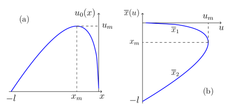
For definiteness, we will consider physical systems with and negative dispersion () which support “bright” soliton solutions in the form of humps of the variable propagating along the background with . We assume that the initial distribution is a smooth function and belongs to the simple-wave type of unidirectional propagation. Its dispersionless evolution according to Eq. (5) leads to steepening of the front so that the wave breaks at some moment of time. To simplify the notation, we take as a wave-breaking moment and choose a localized form of the initial pulse with for and outside this interval. The initial profile has a single maximum at some point (see Fig. 1(a)).
After wave breaking moment a DSW appears and in the Gurevich-Pitaevskii approach the wave number of the locally periodic modulated wave is considered in Whitham approximation as one of the modulation variables, so that presents “a density of waves” within the DSW. Hence the number of waves spanned by DSW is equal to
| (9) |
where we assume that and denote the coordinates of the small-amplitude and soliton edges, correspondingly. Evolution of obeys the number of waves conservation law (Ref. whitham, )
| (10) |
where is the frequency of the periodic travelling wave solution, is its phase velocity. The coordinate corresponds to the position of the leading soliton whose motion along a smooth background does not change . On the contrary, at the small-amplitude edge the wave number is not equal to zero and here we have a flux of waves into the DSW region.
Our starting point is an important remark made by Gurevich and Pitaevskii in Ref. gp-87, that since the small-amplitude edge of the DSW propagates with the group velocity
| (11) |
of the wave at this edge, where is the wave frequency of a linear wave propagating along the background with the amplitude , differs from the phase velocity
| (12) |
of a linear wave, then the length of DSW increases at this edge by in the time interval , so that the number of waves inside DSW increases with time as
| (13) |
Up to the sign, this expression can be regarded as a Doppler-shifted frequency representing the flux of waves into the DSW region. If we integrate the above formula upon time from the wave breaking moment to , then we get the following formula for the number of solitons (see Ref. kamch-20b, )
| (14) |
All the parameters in the integrand are to be calculated at the small-amplitude edge of the DSW at the moment of its evolution.
In Whitham’s approximation, a typical wavelength inside a DSW is much smaller than the size of the whole DSW and this corresponds to the quasi-classical approximation of wave propagation. At the small-amplitude edge the wave is linear and the well-known Hamilton’s optico-mechanical analogy (see, e.g., Ref. lanczos, ) can be applied to propagation of the wave packet moving along the path of the small-amplitude edge. According to this analogy, the motion of this edge can be interpreted as a motion of a classical particle with momentum and Hamiltonian . Then the integrand in (14) is interpreted as a Lagrangian of this classical particle and the integral is equal to the action produced by such a particle during its motion:
| (15) |
Thus, our task is to develop the Hamilton theory of propagation of the small-amplitude edge, extend it to the soliton edge, and to calculate asymptotic number of solitons with the use of Eq. (14).
III General theory
Now we take into account that the dependence of the Hamiltonian on the coordinate of the particle is carried on via the dependence of the background simple wave along which the small-amplitude short wavelength perturbation of DSW propagates at this edge. Evolution of , on the contrary to the short wavelength propagation of the wave packet perturbation, is determined by the dispersionless hydrodynamic approximation of simple-wave type, so that obeys the equation (5). This Hopf equation for the simple-wave evolution can be easily solved for a given initial distribution (see, e.g., Ref. Whitham-74, ),
| (16) |
where is the function inverse to the initial distribution . If we consider initial pulses in the form of a localized hump (see Fig. 1(a)) then the inverse function consists of two branches and (see Fig. 1(b)) and Eq. (16) determines in an implicit form the dependence for each branch.
The specific dependence of the Hamiltonian on and via the solution (16) of Eq. (5) leads to important consequences. In particular, the Hamilton equations
| (17) |
together with Eq. (5) give at once
and their ratio yields the equation
| (18) |
obtained by El in Ref. el-05, . Here the right-hand side depends only on and , so its solution gives
| (19) |
where is the integration constant. The value corresponds to the initial moment of DSW formation when it shrinks to a point in the Gurevich-Pitaevskii approach, that is the small-amplitude edge merges here with the soliton edge where . This determines the boundary condition
| (20) |
for Eq. (18) and specifies the value of the integration constant along the small-amplitude edge path. After such a specification, the wave number depends solely on . As a result, if we consider the evolution of the pulse with a step-like initial condition , then the solution gives us the value of the wave number at the small-amplitude edge propagating along the constant background and, hence, the velocity of its propagation. This approach suggested by El, Ref. el-05, , permitted one to solve a number of interesting problems with step-like initial conditions, Refs. el-05, ; egs-06, ; egkkk-07, ; ep-11, ; lh-13, ; hoefer-14, ; ckp-16, ; hek-17, ; ams-18, .
The solution (19) satisfying the initial condition (20) describes the motion of the wave packet (its ray) at the small-amplitude DSW edge. Apparently, the Hamilton equations (17) have more general character and describe the motion of wave packets along the background with arbitrary initial conditions. Since along each ray found in this way we have , then the variable
| (21) |
defined implicitly by Eq. (19) must satisfy the equation . Combining this equation with Eq. (5), we arrive at the system
| (22) |
with characteristic velocities equal to the limiting Whitham velocities at the small-amplitude edge. Thus, Eqs. (22) comprise continuation of the Whitham equations on a smooth part of the pulse and at the small-amplitude edge of the DSW the variable can be regarded as a Riemann invariant of the Whitham equations in this limit. Obviously, the system (22) has a very general nature and it often arises in description of the problem of interaction of linear wave packets with mean flow (see, e.g. Ref. ceh-19, and references within). It is worth noticing that in our approach the expression (21) is obtained by means of solving Eq. (18) rather then by diagonalization of Eqs. (5) and (10) although both methods are equivalent, of course.
Evidently, a similar reduction of the Whitham equations must exist at the soliton edge of DSW and the question is how to find the Riemann invariant which corresponds to the characteristic velocity equal to the speed of the leading soliton in DSW. A hint to answering this question can be found in an old remark of Stokes fist published in §252 of the book Ref. lamb, and later reproduced in the form of the letter to Lamb in Ref. stokes, . Stokes noticed that propagation of the small amplitude soliton’s tails (“outskirts” according to his terminology) is governed by the same linearized equations that are used for description of propagation of linear travelling waves, so that the expression for the linear wave is replaced by the expression for the tail at . This means that if we make the replacement in the dispersion law for linear waves and define
| (23) |
then the soliton velocity is given by
| (24) |
where has the physical meaning of the inverse half-width of soliton. This remark turned out to be very useful both in concrete studies of nonlinear wave propagation (see, e.g., Refs. ai-77, ; dkn-03, ) and in the theory of DSWs for non-completely-integrable equations (see Refs. el-05, ; egs-06, ; egkkk-07, ; ep-11, ; lh-13, ; hoefer-14, ; ckp-16, ; hek-17, ; ams-18, ).
We assume that the same replacement transforms Eq. (21) into the Riemann invariant
| (25) |
for the reduction
| (26) |
of the Whitham equations at the soliton edge of DSW. Our assumption is confirmed by checking its validity for the completely integrable equations with known Whitham equations in the Riemann diagonal form (see Appendix A). It is easy to check that this transformation casts the Hamilton equations (17) to the form
| (27) |
and again these equations together with the first Eq. (26) yield
| (28) |
Under certain assumptions, this equation was derived by El, Ref. el-05, , from the number of waves conservation law (10).
By construction, the invariant is constant along trajectories defined as solutions of Eqs. (27), so these trajectories can be regarded as paths of solitons with fixed values of . However, changes along the path of the soliton edge determined by the solution of the equation
| (29) |
Apparently, this leading soliton path should be an envelope of paths of solitons with fixed values of . In a sense, at each moment of time the leading soliton is represented by an instant location of some soliton having invariant when it touches the curve representing the path of the soliton edge of DSW. In fact, this mechanism of edge formation as envelopes functions applies to the general form of DSW appearing after wave breaking including its small-amplitude edge. In such general situations the Whitham system does not reduce to one (for step-like initial conditions) or two (for quasi-simple DSWs propagating into the quiescent medium) equations and we do not know beforehand the value of the corresponding edge Riemann invariant or . This qualitative picture of DSW evolution agrees with known particular solutions of Whitham equations for the KdV case which describe evolution of shocks after wave breaking of quadratic and cubic initial profiles (see Appendix B).
So far an initial distribution was assumed to be quite arbitrary. Now we turn to the case of localized initial pulse shown in Fig. 1(a), so that it evolves into solitons. To estimate the integral in Eq. (14) and to find , we need to trace the variation of with time at the small-amplitude edge for the general form of the initial simple-wave pulse. This can be achieved by means of the following reasoning (see Refs. kamch-19, ; kamch-20, ). The small-amplitude edge propagates with the group velocity (11), that is during the time interval it moves to the distance . Since this path lies on the surface of the dispersionless solution, the relation must be compatible with Eq. (16) representing this surface. For a parametric representation and of the small-amplitude path, the differentiation of (16) with respect to and elimination of yields the equation
| (30) |
This linear differential equation can be easily solved with the initial condition at what gives us the dependence of time on for the period of evolution when the small-amplitude edge propagates along the first branch of the dispersionless solution corresponding to . After the moment when reaches the time , we have to solve Eq. (30) with the initial condition at and this gives us the dependence corresponding to propagation of the small-amplitude edge along the second branch of the dispersionless solution. As a result, we obtain the function for the total process of the pulse evolution and this function together with the already known functions and permit us to calculate the number of solitons with the use of Eq. (14). In concrete situations such a calculation can often be done without much difficulty and we shall illustrate the method by a simple example in the next section.
IV Example
We consider here formation of solitons from a pulse whose evolution is governed by the generalized KdV equation
| (31) |
which under certain conditions for , , has periodic and soliton solutions (see Ref. el-05, ). Linearization of this equation yields the dispersion law of linear waves
| (32) |
so that Eq. (18) reduces to
and its solution with the boundary condition Eq. (20) has the form (see Ref. el-05, )
| (33) |
Consequently, the group velocity at the small-amplitude edge propagating along background with the amplitude is equal to . Then Eq. (30) becomes
| (34) |
and for two branches shown in Fig. 1(b) its solution reads (see Ref. kamch-19, )
| (35) |
Substitution of these expressions into Eq. (14) leads after simple transformations to the formula
| (36) |
Here the double integral reduces to the ordinary one by means of evident integration by parts with account of , so that we get the final expression
| (37) |
Remembering the formula (33) for the wave number, we obtain
| (38) |
The expression Eq. (38) agrees with asymptotic formulas for the number of solitons known for completely integrable equations and similar calculations for some other non-completely integrable equations lead to the final expressions which can also written in the form (38) what indicates its generality. The general proof of this expression was suggested in Refs. egkkk-07, ; egs-08, on the basis of extension of the notion of the DSW wave number beyond the DSW region. In the next Section we present modification of this proof which clarifies some its important points.
V Formula for the number of solitons
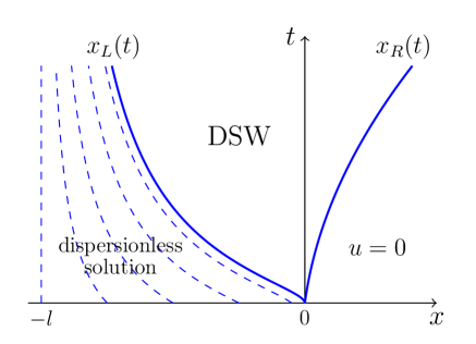
The pulse evolved from the initial distribution depicted in Fig. 1 consists in the Gurevich-Pitaevskii approximation from three parts: on the right of the soliton edge we have the quiescent medium with , the DSW is located between the two edges , and on the left of the small-amplitude edge we have the dispersionless solution (see Fig. 2). The smooth evolution of the pulse outside DSW obeys Eq. (5) whose solution is given in implicit form by Eqs. (16) for two branches and . Linear wave packets can propagate along this smooth background and paths of these packets are given by solutions of the Hamilton equations (17) for certain choice of initial conditions. We know that at the small-amplitude edge the limiting Riemann invariant of the Whitham equations can be defined and its value here is equal to . This equality can be regarded as an expression of the Gurevich-Meshcherkin assumption (see Ref. gm-84, ) that in quasi-simple DSWs the value of preserved dispersionless Riemann invariant is transferred through a DSW. This means that we can define an additional Riemann invariant in the smooth region as an extension of one of the limiting Riemann invariants of Whitham equations to the whole dispersionless region. Thus, in the dispersionless region we have and, consequently, after substitution of this value into Eq. (19), we obtain the extension of the function to the smooth region which yields distribution of wave numbers as an extension of DSW’s wave number at the small-amplitude edge to the whole smooth region (see Fig. 2). One can say that this is a specific property of the Whitham approximation: although the amplitude of oscillations is equal here zero in this approximation, the notion of the wavelength of waves, entering into the DSW region, still has physical meaning. Obviously, for since here and . Solutions of the equation
| (39) |
with the initial condition , , give us a family of rays along which wave packets propagate when they are radiated from points with the carrying wave numbers ; they are shown by dashed lines in Fig. 2. In particular, the ray radiated from the wave breaking point gives us the path of the small-amplitude edge of the DSW. We denote this path as .
Now we define the number of waves corresponding to the defined above distribution :
| (40) |
It complements the number of waves entered into the DSW region up to the moment of time (see Eq. (9)). The number changes with time according to Eq. (13), so let us calculate the derivative of with respect to :
We can substitute Eq. (39) with into the first term. Then, by definition the function satisfies the number of waves conservation law (10) and this statement can easily be checked with the help of Eqs. (5) and (18), so in the second term the integrand can be replaced by , and after integration we get
| (41) |
This is equal to Eq. (13) with opposite sign, that is . At last, since in the limit we have , and for we have , and , we arrive at the final formula for the number of solitons
| (42) |
where the function is the solution of Eq. (18) with the boundary condition Eq. (20). The presented here proof of Eq. (42) provides an explicit construction of the function for wave numbers in the smooth region of the pulse introduced earlier in Refs. egkkk-07, ; egs-08, . The formula (42) was confirmed by numerical solutions of nonlinear wave equations and it agrees very well with the results of recent experiments presented in Ref. maiden-20, .
Under some additional assumptions, the asymptotic distribution of solitons parameters was obtained in Ref. egs-08, .
VI Conclusion
The notion of quasi-simple DSWs was first introduced in Ref. gkm-89, for the KdV equation case as the shocks with only two Riemann invariants changing along them. In this paper, we generalized this notion to nonlinear wave situations with wave breaking of simple waves, so that, according to Gurevich-Meshcherkin conjecture, one dispersionless Riemann invariant has the same value at both edges of the DSW under consideration. This definition is not limited to the class of completely integrable equations and is applicable to any nonlinear wave equations admitting propagation of solitons. As follows from the Gurevich-Pitaevskii remark made in Ref. gp-87, on the number of waves entering into the DSW region in a unit of time, propagation of the high-frequency wave packet at the small-amplitude edge of DSW satisfies the Hamilton equations with the linear dispersion law playing the role of the Hamiltonian, Ref. kamch-20b, . This system of Hamilton equations is coupled with the Hopf equation for evolution of the background field what results in the diagonal form of the Whitham equations at the DSW edges.
Long ago G. G. Stokes remarked in Refs. stokes, ; lamb, that the expression for soliton’s velocity can be obtained from the dispersion law for linear waves because the tails of a soliton obey the same linearized equations as the small-amplitude travelling waves. We generalize here this observation to the symmetry relationships between equations at the small-amplitude and soliton edges:
| (43) | |||||
| (44) | |||||
| (45) | |||||
| (46) | |||||
| (47) | |||||
| (48) |
is the wave number at the small-amplitude edge, is in the soliton’s inverse half-width at the soliton edge, and at both edges the background field obeys the same equation
| (49) |
Equations (48) and (49) comprise the limiting Whitham equations at the DSW edges for the Riemann invariants or , respectively.
Generally speaking, paths of small-amplitude and soliton edges of DSW are represented by envelopes of characteristics of Whitham equations and their finding is not an easy task in non-completely-integrable case. Important exceptions are the situations with initial step-like distributions when velocities of both edges can be found (see Ref. el-05, ) and a quasi-simple DSW propagating into a quiescent medium when the path of one its edge can be calculated and the asymptotic velocity of the other edge can be found in the case of localized pulses (see Refs. kamch-19, ; kamch-20, ).
In case of localized quasi-simple DSW propagating into a quiescent medium and evolving into a train of solitons, the asymptotic formula for their number can be derived with the use of Gurevich-Pitaevskii theorem on the number of oscillations entering into the DSW region. The resulting formulas agree with the expression derived in Refs. egkkk-07, ; egs-08, .
At last, although we considered here a concrete problem of evolution of quasi-simple DSWs, some results can be applied to other problems of interaction of linear modulated waves with mean flow; see, e.g., Ref. ceh-19, .
To sum up, the presented in this paper theory unifies the previously obtained result into a consistent approach applicable to a wide class of quasi-simple DSWs.
Acknowledgements.
I am grateful to G. A. El, N. Pavloff and L. P. Pitaevskii for useful discussions. This study was funded by RFBR, project number 20-01-00063.Appendix A Limiting Whitham equations: KdV equation case
We shall consider the KdV equation
| (50) |
for which the Whitham system modulation equations can be written in diagonal form with Riemann invariants . Near the small-amplitude edge a DSW is approximated by the small-amplitude solution (see, e.g., Ref. kamch-20b, )
| (51) |
where the Riemann invariants obey the limiting Whitham equations
| (52) |
As follows from Eq. (51), the background field and the wave number are expressed in terms of by the formulas
| (53) |
Hence, we get and Eqs. (54) take the form
| (54) |
which coincides with the system Eqs. (22) with account of the dispersion law
| (55) |
of linear waves for a linearized Eq. (50).
Now, at the opposite edge of DSW the leading soliton has the form
| (56) |
and the Whitham equations reduce to
| (57) |
We get expressions for the background field and the inverse half-width of soliton from Eq. (56),
| (58) |
so and Eqs, (57) take the form
| (59) |
coinciding with Eqs. (26) with account of
| (60) |
Similar symmetry between equations for the DSW’s edges can be proved for other completely integrable equations.
Appendix B Paths of DSW edges as envelopes
First we consider situation with wave breaking of a parabolic pulse with which belongs to the quasi-simple type. In the KdV equation theory, at the soliton edge with the Whitham system Eqs. (57) reduces to
| (61) |
and its global solution becomes (see Ref. gkm-89, ; kamch-20b, )
| (62) |
These are the characteristic curves near the soliton edge and for their envelope the differentiation of Eq. (62) with respect to gives the relation . Then and the path of the soliton edge is given by
| (63) |
in agreement with the known result (see Ref. gkm-89, ; kamch-20b, ).
Now we turn to a more complicated situation with the generic Gurevich-Pitaevskii problem on wave breaking of a cubic initial profile with . In this case all three Riemann invariants are changing within the DSW and the global solution of Whitham equations was found in Ref. potemin, (see also Ref. kamch-20b, ). At the small-amplitude edge it reduces to
It was shown that at this edge we have , , so the above equation becomes
| (64) |
and along envelope of these curves we get . Then the group velocity is equal to and integration of yields for the small-amplitude path the formula
| (65) |
in agreement with Refs. potemin, ; kamch-20b, .
In a similar way at the soliton edge the global solution gives
and it was shown that here , , hence this equation becomes
| (66) |
Along envelopes of these curves we get , , so integration of yields
| (67) |
again in agreement with Refs. potemin, ; kamch-20b, .
These examples demonstrate essential difference between step-like initial conditions, simple wave pulse propagating into a quiescent medium, and the general simple wave initial pulse.
References
- (1) S. C. Gardner, J. M. Greene, M. D. Kruskal, R. M. Miura, Phys. Rev. Lett., 19, 1095 (1967).
- (2) V. I. Karpman, Phys. Lett. A, 25, 708 (1967).
- (3) A. V. Gurevich and L. P. Pitaevskii, Zh. Eksp. Teor. Fiz., 65, 590 (1973) [Sov. Phys.-JETP, 38, 291 (1974)].
- (4) G. B. Whitham, Proc. Roy. Soc. London, A 283, 238 (1965).
- (5) A. V. Gurevich, A. L. Krylov, and N. G. Mazur, Zh. Eksp. Teor. Fiz., 95, 1674 (1989) [Sov. Phys. JETP, 68, 966 (1989)].
- (6) C. H. Su, C. S. Gardner, J. Math. Phys., 10, 536 (1969).
- (7) A. V. Gurevich, A. L. Krylov, G. A. El, Zh. Eksp. Teor. Fiz., 98, 1605 (1990) [Sov. Phys. JETP, 71, 899 (1990)].
- (8) L. D. Landau and E. M. Lifshitz, Fluid Mechanics, Pergamon, Oxford (1987).
- (9) A. V. Gurevich, A. P. Meshcherkin, Zh. Eksp. Teor. Fiz., 87, 1277 (1984) [Sov. Phys. JETP, 60, 732 (1984)].
- (10) A. V. Gurevich and L. P. Pitaevskii, Zh. Eksp. Teor. Fiz., 93, 871 (1987) [Sov. Phys.-JETP, 93, 871 (1987)].
- (11) A. M. Kamchatnov, “Gurevich-Pitaevskii problem and its development”, Phys. Usp., accepted; DOI: 10.3367/UFNe.2020.08.038815.
- (12) C. Lanczos, The Variational Principles of Mechanics, (University of Toronto Press, Toronto, 1962).
- (13) G. B. Whitham, Linear and Nonlinear Waves, (Wiley Interscience, New York, 1974).
- (14) G. A. El, Chaos, 15, 037103 (2005).
- (15) G. A. El, R. H. J. Grimshaw, N. F. Smyth, Phys. Fluids, 18, 027104 (2006).
- (16) G. A. El, A. Gammal, E. G. Khamis, R. A. Kraenkel, A. M. Kamchatnov, Phys. Rev. A 76, 053813 (2007).
- (17) J. G. Esler, J. D. Pearce, J. Fluid Mech., 667, 555 (2011).
- (18) N. K. Lowman, M. A. Hoefer, J. Fluid Mech., 718, 524 (2013).
- (19) M. A. Hoefer, J. Nonlinear Sci., 24, 525 (2014).
- (20) T. Congy, A. M. Kamchatnov, N. Pavloff, SciPost Phys. 1, 006 (2016).
- (21) M. A. Hoefer, G. A. El, A. M. Kamchatnov, SIAM J. Appl. Math., 77, 1352 (2017).
- (22) X. An, T. R. Marchant, N. F. Smyth, Proc. Roy. Soc. London A 474, 0278 (2018).
- (23) T. Congy, G. A. El, M. A. Hoefer, J. Fluid Mech., 875, 1145 (2019).
- (24) H. Lamb, Hydrodynamics, (Cambridge University Press, Cambridge, 1994).
- (25) G. G. Stokes, Mathematical and Physical Papers, Vol. V, p. 163 (Cambridge University Press, Cambridge, 1905).
- (26) O. Akimoto and K. Ikeda, J. Phys. A: Math. Gen. 10, 425 (1977).
- (27) S. A. Darmanyan, A. M. Kamchatnov, M. Neviére, Zh. Eksp. Teor. Fiz., 123, 997 (2003) [JETP, 96, 876 (2003)].
- (28) A. M. Kamchatnov, Phys. Rev. E 99, 012203 (2019).
- (29) A. M. Kamchatnov, Teor. Mat. Fiz., 202, 415 (2020) [Theor. Math. Phys., 202, 363 (2020)].
- (30) G. A. El, R. H. J. Grimshaw, N. F. Smyth, Physica D 237, 2423 (2008).
- (31) M. D. Maiden, N. A. Franco, E. G. Webb, G. A. El, M. A. Hoefer, J. Fluid Mech., 883, A10 (2020).
- (32) G. V. Potemin, Russian Math. Surveys, 43, 39 (1988).