Thermal conductivity in one-dimensional nonlinear disordered lattices: Two kinds of scattering effects of hard-type and soft-type anharmonicities

With the above model and simulation setups, we now are able to study the $\xi$-dependence of thermal conductivity $\kappa$. Numerically, there are two main approaches to achieve this. The first one is based on the Green-Kubo formula (GK1, ; GK2, ; Kubo1991, )

where $k_{B}$ is the Boltzmann constant (set to be $1$), $C_{JJ}(t)=\langle J(0)J(t)\rangle$ is the time autocorrelation of heat currents, where $J=\sum_{i}\frac{1}{2}(\dot{x}_{i+1}+\dot{x_{i}})\frac{\partial H(x_{i+1}-x_{i})}{\partial x_{i}}=\sum_{i}-\frac{1}{2}(\dot{x}_{i+1}+\dot{x}_{i})(x_{i+1}-x_{i})$ is the total heat current [$\dot{x}_{i}=\frac{dx_{i}(t)}{dt}$] (PR2003, ; AP2008, ) and $\langle\cdot\rangle$ denotes the ensemble average. To obtain $C_{JJ}(t)$, the system is first thermalized to a given temperature with the Langevin heat baths, which are then removed after the equilibrium state is eventually reached. Finally, $\kappa$ can be measured through the Green-Kubo integration from Eq. (3). For each $C_{JJ}(t)$, we take average over $24$ different initial conditions.

The second method is from the direct molecular dynamic simulations of nonequilibrium states. In this method, two ends of the system are first connected to two Noose-Hoover heat baths with temperatures $T_{+}=0.6$ and $T_{-}=0.4$ (the average temperature of the system is then $T=0.5$), respectively. These thermal baths will drive the system to a nonequilibrium steady state, and also produce a well-behaved temperature gradient that results in heat current flowing across the system. Finally, the thermal conductivity $\kappa$ can be calculated through the Fourier law $\kappa=jN/(T_{+}-T_{-})$ with $j$ being the heat current density flowing through each particle.

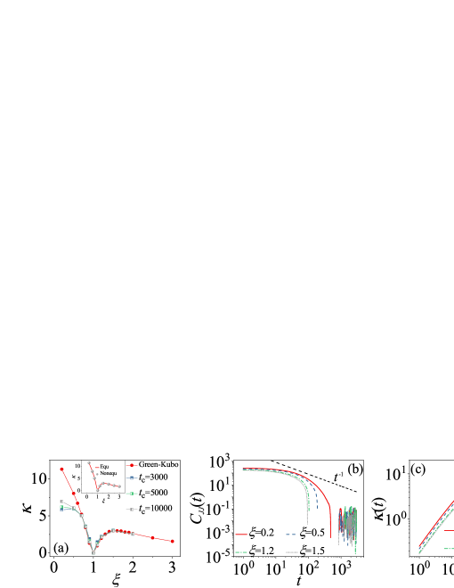
Figure 1(a) shows our main results of $\xi$-dependence of $\kappa$. As can be seen in the inset, both the equilibrium and nonequilibrium approaches give quantitatively the same results. First, the harmonic disordered model ($\xi=1$) has a minimal $\kappa=0$ because in this case all the phonon modes become Anderson localized as expected. Second, in the HT type model a usual nonmonotonous $\xi$-dependence of $\kappa$ can be identified (Ourwork2020, ), i.e., as $\xi$ increases from $\xi=1$ (the on-site potential becomes hard), $\kappa$ first increases, then reaches its maximum at certain $\xi$ value, and finally decreases. This nonmonotonous behavior has been attributed to the delocalization and re-localization of the Anderson modes induced by the combined effects of disorder and nonlinearity (Ourwork2020, ). Bearing this in mind, let us now turn to the results of the ST type model. Interestingly, as $\xi$ decreases from $\xi=1$, i.e., the on-site potential becomes soft, the nonmonotonous behavior no longer exists. $\kappa$ monotonously increases with the decrease of $\xi$, implying that only delocalization processes appear in the ST systems, which is quite different from the counterpart HT systems.

Some results from the equilibrium approach, e.g. the heat current auto-correlations $C_{JJ}(t)$ of $\xi=0.2,0.5,1.2$, and $1.5$ are shown in Fig. 1(b). All of the correlations decay faster than $t^{-1}$, indicating the possible convergence to derive $\kappa$ by using the Green-Kubo formula. This is also consistent with the known results of normal heat conduction in momentum nonconserving systems obeying the Fourier law (PR2003, ; AP2008, ; Zhao1998, ). The corresponding integration of Eq. (3) for each $\xi$ is presented in Fig. 1(c), which further confirms our conjecture of the convergence.

We next present the predictions by the unified formula (NC2019, ; NP2019, ) to see if they can be validated by our 1D disordered models with both HT and ST on-site potentials, and especially how the ST anharmonicity plays a role in the unified formula. For facilitating the comparison with the simulation results, here we only focus on the unified formula based on QHGK method proposed in (NC2019, ). When applying to the 1D model the formula reads:

where $v_{nm}$ and $\tau_{nm}$ are the generalized group velocity and the lifetime of Anderson modes, respectively; $\omega_{n}$, $e_{n}$, and $\gamma_{n}$ is the frequency, eigenvector, and decay rate of the $n$th normal mode, respectively; $R_{i}^{o}$ is the equilibrium position of the $i$th particle, and $\Phi_{ij}=(\frac{\partial^{2}H}{\partial x_{i}\partial x_{j}})_{0}$ is the element of the force-constant matrix (here the subscript $0$ indicates the equilibrium position of the reference particle).

To implement this formula, one may simply set $x_{i}=A_{i}\exp(-\rm i\mathrm{\omega_{n}}\mathrm{t})$, which enables us to linearize the motion equation of particles such that the dynamic matrix can be diagonalized. Let $e_{n}^{i}$ and $\omega_{n}$ be the $n$th normalized eigenvector and eigenvalue of the dynamic matrix, and the projection of the motion onto the $n$th Anderson mode be $Q_{n}(t)=\sum_{i}^{N}\sqrt{m_{i}}x_{i}(t)e_{n}^{i}$ and $P_{n}(t)=\sum_{i}^{N}\sqrt{m_{i}}\dot{x}_{i}(t)e_{n}^{i}$ with $n=1,\ldots,N$ and $P_{n}$ and $Q_{n}$ being the canonical momentum and canonical coordinate, respectively. Here we only present the predictions of formula (III.2) in Fig. 1(a), leaving the details of obtaining $\Phi_{ij}$, $\gamma_{n}$, etc. for calculating $\kappa$ in the following sections.

As shown in Fig. 1(a), the unified formula (III.2) gives an accurate prediction of $\kappa$ for the HT disordered model even when the system is strongly anharmonic, for example $\xi=2$. However, for the ST disordered model, this formula only holds for the range $0.7\leqslant\xi<1.0$. The predicted values of $\kappa$ seem to be lower than those from direct dynamic simulations when $\xi<0.7$, even if we have further increased the integration time to obtain the decay rate of the Anderson normal modes [see Fig. 1(a) and the detailed calculations below]. These results further demonstrate that the ST anharmonic disordered systems is beyond the scope of the unified formula.

The matrix $\Phi_{ij}$ in the QHGK method (NC2019, ) is composed of force-constants. However, as mentioned in introduction, one cannot use the origin harmonic force-constant to construct the dynamic matrix. Instead an effective force-constant $k_{eff}$, induced by both HT and ST anharmonicities, should be first given when applying the QHGK method. Here we present the analytical results of SCPT for deriving $k_{eff}$, and then provide the numerical measure from direct dynamic simulations.

The basic idea of SCPT is to use a harmonic Hamiltonian $H_{0}$ to approximate a general Hamiltonian $H$. Then, by minimizing the free energy, one can get a self-consistent equation for $k_{eff}$ (PRB1991-JR, ; PRB1992-JR, ; PRE1993-Dauxois, ; PRE2008-He, ; PRE2007-Nianbei, ; PRE2014-Nianbei, ; PRE2021-He, ). Considering a general Hamiltonian $H$, SCPT tells us that one can use an equivalent harmonic Hamiltonian $H_{0}$ so that the free energy is minimized, i.e.

where $F$, $F_{0}$, and $\langle H-H_{0}\rangle_{0}$ are the free energies of the original system, the effective harmonic system, and the average of their Hamiltonian difference, respectively. Note that the average is taken over the equivalent harmonic system and the minimization is taken on $\langle H-H_{0}\rangle_{0}$. Further, considering the statistical equivalence of particles in lattice systems, it is actually feasible to minimize $\langle H-H_{0}\rangle_{0}$ for a single particle.

For our focused Hamiltonian (1), the anharmonicity only appears in the on-site potential, and $H_{0}=\sum_{i}\frac{p_{i}^{2}}{2m_{i}}+\frac{1}{2}(x_{i+1}-x_{i})^{2}+\frac{k_{eff}}{2}x_{i}^{2}$. To calculate $\langle H-H_{0}\rangle_{0}$, we first write the on-site potential in Hamiltonian (1) in an inverse form

where $\langle x^{2}\rangle_{0}=\frac{\int x^{2}e^{-\frac{k_{eff}}{2k_{B}T}x^{2}}dx}{\int e^{-\frac{k_{eff}}{2k_{B}T}x^{2}}dx}=\frac{T}{k_{eff}}$. Now let $y=\langle x^{2}\rangle_{0}$, $\langle H-H_{0}\rangle_{0}$ can be rewritten as $f=-\frac{1}{2}\xi y+\frac{1}{2}\frac{1}{\frac{1}{y}+\frac{1-\xi}{1+\xi y}}$. To satisfy the Eq. (5), one requires that $\frac{\partial f}{\partial y}=0$, from which a self-consistent equation $k_{eff}^{3}+(2T-1)k_{eff}^{2}+(T^{2}-2\xi T)k_{eff}-\xi T^{2}=0$ can be obtained. Finally substituting the given temperature $T=0.5$ into this self-consistent equation, one obtains an explicit self-consistent relation between $k_{eff}$ and $\xi$:

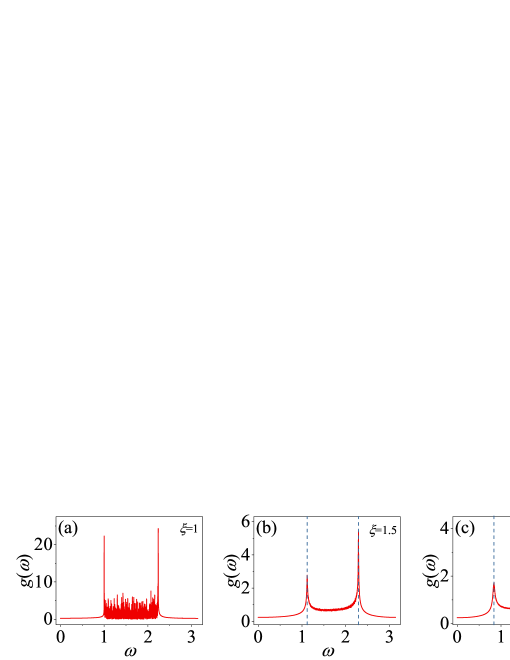
Eq. (7) provides an analytical relation to derive $k_{eff}$. Here it is also desirable to find $k_{eff}$ directly from simulations. For this purpose, we now consider the density of states (DOS) $g(\omega)$ of the system. As it is well known that in a pinned harmonic homogeneous system [with Hamiltonian $H=\sum_{i}^{N}\frac{p_{i}^{2}}{2}+\frac{1}{2}(x_{i+1}-x_{i})^{2}+k_{eff}\frac{1}{2}x_{i}^{2}$], the minimal and maximal frequencies are $\omega_{min}=\sqrt{k_{eff}}$ and $\omega_{max}=\sqrt{4+k_{eff}}$, respectively. This helps us obtain $k_{eff}$ numerically. In practice, DOS can be obtained via Fourier transformation of the particle velocity auto-correlation. Some typical results of DOS for different $\xi$ are shown in Fig. 2. For a harmonic system [$\xi=1$, see Fig. 2(a)], there are actually two peaks located at $\omega=1$ and $\omega\simeq 2.236$, respectively, indicating $k_{eff}=1$. For the HT anharmonic systems [for example $\xi=1.5$, see Fig. 2(b)], the frequency shift of the phonon modes happens, while in the case of ST anharmonicsystems [e.g., $\xi=0.5$, see Fig. 2(c)], the softening of the normal modes (the decrease of $\omega_{n}$) takes place. Both evidences enable us to measure $k_{eff}$ caused by anharmonic on-site potential for the corresponding disordered systems.

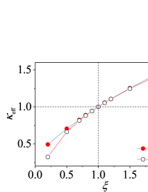
In Fig. 3 we compare the results of $k_{eff}$ for different $\xi$ both from SCPT and from our direct simulation measurements based on DOS. As can be seen, in a fairly wide range of $\xi$ around $\xi=1$, both approaches give consistent results. However, as the on-site potential becomes soft, some discrepancy can be identified. This discrepancy becomes more significant when we look at the ST model (e.g. from $\xi=0.5$ and below, Fig. 3). Therefore for a more complicated ST anharmonic disordered model system, one should be more cautious when applying the unified formula to predict $\kappa$. Viewing all of these, in the following we shall include $k_{eff}$ from our direct dynamic simulation measurements in the practical calculations in Eq. (III.2).

With $k_{eff}$, the eigenvalue $\omega_{n}$ and eigenvector $e_{n}$ of an Anderson mode can be immediately extracted from diagonalizing the dynamic matrix. For applying the QHGK formula (NC2019, ), we still need to know the decay rate $\gamma_{n}$. In dynamic simulations, $\gamma_{n}$ can be measured by the time evolution of the equilibrium energy-energy autocorrelation of a single Anderson mode, defined by

where $\Delta E_{n}(t)=E_{n}(t)-\langle E_{n}\rangle$ with $E_{n}=\frac{1}{2}(P_{n}^{2}+\omega_{n}^{2}Q_{n}^{2})$ being the instantaneous energy of the Anderson mode $n$. Therefore, under the single-mode relaxation approximation, the $n$th mode energy decay rate $\Gamma_{n}$ (PRB1986-Ladd, ) is determined by

Note that mathematically $\gamma_{n}=\Gamma_{n}/2$ since in principle the $n$th mode decay rate $\gamma_{n}$ should be measured by a similar definition $\frac{1}{\gamma_{n}}=\lim\limits_{t_{c}\rightarrow\infty}\int_{0}^{t_{c}}C_{n}^{Q}(t)dt$ with $C_{n}^{Q}(t)=\frac{\langle\Delta Q_{n}(0)\Delta Q_{n}(t)\rangle}{\langle\Delta Q_{n}(0)\Delta Q_{n}(0)\rangle}$. Measuring $C_{n}^{E}(t)$, however, is just for facilitating the numerical simulations.

The inverse of $\Gamma_{n}$ is called the lifetime of the $n$th Anderson mode. To obtain a finite $\Gamma_{n}$ from the integration in Eq. (9), $C_{n}^{E}(t)$ should be a fast decay function. If the decay of $C_{n}^{E}(t)$ were not fast enough, the integration would have become divergent, indicating an infinite lifetime of the normal mode. This means that there is always a part of energy fluctuations locked in the normal localized mode. Given that, in practice it is better to truncate the integration in Eq. (9) at some time cutoff $t_{c}$ (see also Fig. 1) and analyze how the integration changes.

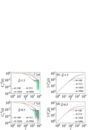
Figures 4(a) and (c) depict the decay of $C_{n}^{E}(t)$ for four typical Anderson modes. Fortunately all these $C_{n}^{E}(t)$ decay faster than $t^{-1}$, indicating a finite lifetime of these modes. These have been numerically verified in Figs. 4(b) and (d). Some observed details are noteworthy, e.g. $C_{n}^{E}(t)$ with $n$ being some number in the middle of mode range (e.g., $n=512$ and $1024$) decays faster than those with $n$ at boundaries (e.g., $n=100$ and $3996$ in our simulations). This indicates that the $512$th and $1024$th Anderson modes have shorter lifetimes than those of the $100$th and $3996$th modes, which is consistent with the previous results observed only in the HT models (Ourwork2020, ).

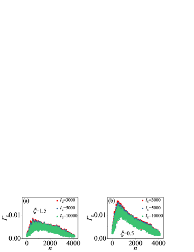
To further study the properties of the ST anharmonic disordered systems, we provide $\Gamma_{n}$ in Fig. 5 for three truncated times $t_{c}$. On the one hand, for all modes, $\Gamma_{n}$ nearly do not change with $t_{c}$, indicating possible convergence of the integration (9); On the other hand, from the results of Figs. 5(a) and (b), the lifetimes of the Anderson modes for the ST anharmonic disordered systems seem shorter than those of the HT ones, implying a stronger delocalization induced by the ST anharmonicities.

From the above direct dynamic simulations via both the equilibrium and nonequilibrium approaches, plus the theoretical QHGK unified formula (NC2019, ), we know that the ST anharmonic disordered systems have larger thermal conductivity $\kappa$ than the counterpart HT systems. In addition, the current QHGK method (NC2019, ), even including the effective force-constant that obtained both from SCPT and direct simulations, is still not able to give a thorough prediction for the ST anharmonic disordered systems. The distinctions from the counterpart HT systems and the invalidity of the predictions seem to be relevant to the same invalidity of SCPT and the shorter lifetime of the Anderson modes in the ST anharmonic disordered systems. To further investigate why the aforementioned methods fail to calculate $\kappa$ of the ST systems, we discuss the localization properties of the normal Anderson modes, characterized by their localization lengths.

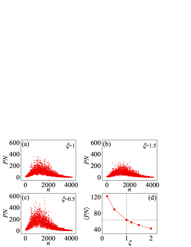
The localization properties of phonon modes can be studied by the participation number $PN$ which is defined by $PN=\frac{(\sum A_{i}^{2})^{2}}{\sum A_{i}^{4}}$ (PN1970, ), where $A_{i}$ is the amplitude of the displacement $x_{i}=A_{i}\exp(-\rm i\mathrm{\omega_{n}}\mathrm{t})$ that we have already substituted into the equations of motion to diagonalize the dynamic matrix. For a normal mode ($\omega_{n}$) in which $A_{i}$ is constant, $PN=N$, which implies a uniform participation of motions for all particles in that mode. This is a sign of delocalization. For a mode whose motions are carried by a single particle, $PN=1$ which indicates the highest degree of localization. Equivalently, $PN$ can be considered as the localization length of the modes and is inversely proportional to the degree of localization since a mode with a smaller localization length corresponds to a higher degree of localization.

Figure 6 depicts $PN$ versus the mode index $n$ for $\xi=1$, $\xi=1.5$, and $\xi=0.5$, respectively. Note that in practice we only need to calculate $\frac{1}{\sum A_{i}^{4}}$ to derive $PN$ due to the normalization of eigenstates $\sum A_{i}^{2}=1$. As can be seen in Figs. 6(a)-(c), the curves of $PN$ versus $n$ are bell-shaped, i.e., the Anderson mode with a middle $n$ value has a relatively larger $PN$ than those with $n$ at boundaries. This implies that the middle $n$th mode of the corresponding homogeneous systems has a larger group velocity than the boundary modes (PSheng, ). Furthermore, a detailed comparison of Figs. 6(a)-(c) shows that the HT potential enhances the Anderson localization while the counterpart ST potential mainly weakens it. From Figs. 6(b) and (c), $PN$ of the ST model is manifestly larger than that of the HT model. This is also supported by the results of the averaged $PN$ ($\langle PN\rangle$) with respect to $\xi$ in Fig. 6(d). This is a crucial distinction between the HT and ST model systems. Such observations are also consistent with the decay rates of localized normal modes as shown in Fig. 5.

Now let us understand more about the results of thermal conductivity shown in Fig. 1(a). For the purely harmonic disordered systems, all the Anderson modes are fully localized and non-interacting, hence $\kappa=0$. For the HT anharmonic disordered systems, on the one hand the HT anharmonic on-site potential brings mode-mode interactions into the system; on the other hand it eventually enhances the localization. Therefore, these two mechanisms compete and finally lead to the nonmonotonous finite $\xi$-dependent $\kappa$. Here $\kappa$ approaches a finite value and can be accurately predicted by the unified formula (III.2). The scenario, however, changes dramatically for the ST anharmonic on-site potential, whose main effect on disordered systems is to delocalize the Anderson modes, similar to the effect of the mode interactions induced by nonlinearity. Combining both effects it results in a stronger monotonous increase of $\kappa$ with respect to $\xi$. As we at present do not know whether there is a upper limit of $\kappa$, and $\kappa$ becomes larger when the anharmonicity keeps increasing, it is hard to predict $\kappa$ by any existing theories when $\xi$ exceeds a certain threshold value.