Thermodynamic engine with a quantum degenerate working fluid
Abstract
Can quantum mechanical thermodynamic engines outperform their classical counterparts? To address one aspect of this question, we experimentally realize and characterize an isentropic thermodynamic engine that uses a Bose-condensed working fluid. In this engine, an interacting quantum degenerate gas of bosonic lithium is subjected to trap compression and relaxation strokes interleaved with strokes strengthening and weakening interparticle interactions. We observe a significant enhancement in efficiency and power when using a Bose-condensed working fluid, compared to the case of a non-degenerate gas. We demonstrate reversibility, and measure power and efficiency as a function of engine parameters including compression ratio and cycle time. Results agree quantitatively with exact interacting finite temperature field-theoretic simulations.
Classical thermodynamic engines have been critical to human technology since the industrial revolution. In the past decade, the capabilities of quantum thermodynamic engines have been explored theoretically [1, 2, 3, 4, 5, 6, 7, 8, 9, 10, 11, 12, 13, 14, 15, 16, 17, 18, 2, 19, 20], and recent years have seen experimental demonstrations of both quantum and nanoscopic classical engines using single ions [21, 22], nuclear spins [23], cold atoms [24, 25, 26], nitrogen-vacancy centers [27], and quantum gases [28, 29]. A natural question is whether quantum phenomena can enhance the performance of a thermodynamic engine [30, 31, 32]. Perhaps the simplest experimental approach to this question — the direct comparison of an engine using a classical working fluid to an equivalent one using a quantum degenerate working fluid — has remained unexplored.
In this work, we experimentally realize and characterize an isentropic thermodynamic engine with a quantum degenerate working fluid. The engine cycle interleaves compression and decompression of an optical trap with Feshbach enhancement and suppression of interparticle scattering to pump energy from a magnetic field to an optical field via a trapped ensemble of ultracold neutral lithium. We observe that quantum degeneracy significantly enhances the output power. We measure the dependence of efficiency and power on cycle time, and investigate the effects on engine performance of compression ratio and interaction strength ratio. Results agree quantitatively with both approximation-free finite temperature interacting numerical simulations and mean-field analytics.
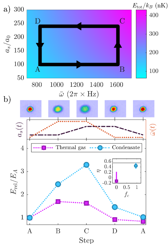
The experiments begin by preparing a Bose-Einstein condensate (BEC) of 300,000 to 1 million 7Li atoms in a far-detuned crossed optical dipole trap with a mean trap frequency Hz, at a temperature of 170 nK, corresponding to a condensate fraction of 0.95. After evaporative cooling to degeneracy, the -wave interparticle scattering length is Feshbach-tuned to 100, where is the Bohr radius. This sets the initial condition (labeled in figures). Interleaved variation of the trap intensity and Feshbach field then execute the thermodynamic cycle illustrated in Fig. 1a. Between steps and (stroke ), the trap power is increased with a functional form such that increases from to at a constant rate. This is the compression stroke of the engine. In stroke , the trap frequency is held constant as the interaction strength is ramped from to a larger value at a constant rate. Subsequently, the trap frequency and then the interactions are ramped linearly back to their initial values. Such a cycle pumps energy between the magnetic and optical control fields, because the work performed by the strongly interacting gas during decompression is not equivalent to the work done to compress the more weakly interacting gas. Performing the strokes of the cycle in the order shown in Fig. 1a results in a net transfer of energy from magnetic to optical fields. Appendix B details an intuitively useful analogy between this isentropic cycle and the Otto heat-engine cycle.
The second-quantized Hamiltonian describing the working fluid includes kinetic, interaction, and potential terms:
| (1) | |||
where is the interaction coupling constant, is the scattering length, is the mass, and is the trap frequency of mode k at time . To measure release energy (defined below) at each step, we first abruptly switch off the trap, quenching to zero the last term of the Hamiltonian . Following 12 ms of free expansion we measure the column-integrated density distribution by absorption imaging and reconstruct the 3D distribution via Abel inversion [33]. After expansion, not only is the initial momentum distribution converted to a position distribution, but also essentially all the initial interaction energy is converted to kinetic energy [34], so the distribution provides a measure of the condensate’s release energy . We report release energies per atom, while plotted powers represent the total engine power.
Engine performance can be characterized by efficiency and power. We define work done on the condensate as positive. As in refs. [7, 12], we define the efficiency
| (2) |
and the power
| (3) |
Here is the work done on the BEC by the field (laser or magnetic) in stroke of the cycle and is the total cycle time.
While we measure the release energy rather than the total energy, thse quantities can be simply related via the Gross-Pitaevskii description of an interacting gas. In the Thomas-Fermi regime, the total energy is given by [35]
| (4) |
where is the chemical potential, , and . The ratio between the total energy and the measured energy is then
| (5) |
Therefore, a power measurement based on release energy will be reduced from the true power by a factor of 2.5, while measured efficiency will give the true value. As shown later, we have verified the validity of these assumptions using approximation-free numerics.
Fig. 1b demonstrates the stark contrast between the behavior of degenerate and non-degenerate gases subjected to similar thermodynamic cycles. The thermal gas is prepared via inhibited evaporation at a small scattering length of 57, resulting in a density of at a temperature of 890 nK. The density of the condensate is , about 33 times larger, at a temperature of 170 nK. Much of this enhancement in density is a direct result of bosonic quantum statistics. While the thermal gas and condensate are prepared at different trap frequencies, the compression ratio is the same for both. As interaction strength increases, the low density of the thermal gas results in a negligible change in release energy, while the Bose-enhanced density of the quantum degenerate sample results in a significant change. The measured efficiency of the engine with a thermal working fluid is consistent with zero, while the measured efficiency of the engine with a quantum degenerate working fluid is , near the maximum theoretical value of 0.55 for this compression ratio.
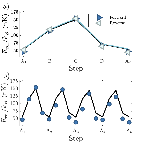
Reversibility can be tested by comparing the results of forward (----) and reverse (----) cycles. Fig. 2a shows the experimental results of such a comparison, demonstrating a high degree of reversibility and confirming that the reverse cycle results in a net transfer of energy from optical to magnetic fields, opposite to the forward cycle. Fig. 2b shows that the same cycle can be performed many times. The repeated return of the condensate to its initial release energy indicates that it can mediate energy transfer between magnetic and optical fields without significant net absorption of energy.
To estimate the degree of adiabaticity, one can apply the Landau-Zener formalism [36] to approximate the probability of low-lying collective excitations [37]. Considering only the ground state and lowest-lying collective excitation, the probability of diabatic passage between them is , where the adiabaticity parameter depends on the energy gap to the nearest excited level. Taking our trap to be approximately axially symmetric, and using the results of [37] with a known ramp speed Hz/ms, we estimate a maximum adiabaticity parameter of for the cycles shown in Figs. 1 and 2, with cycle times of 530 ms.
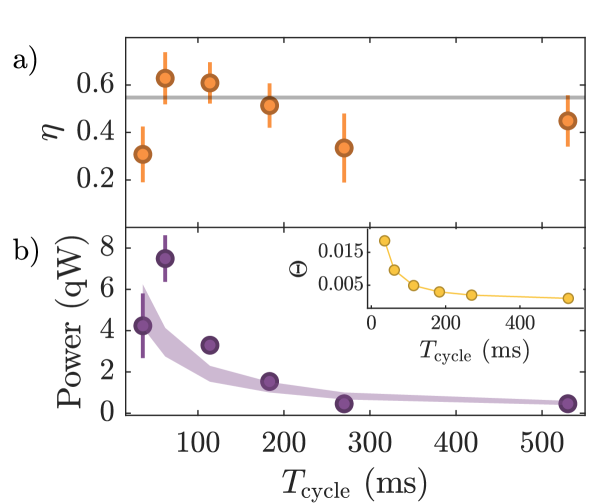
Varying the engine cycle time affects both efficiency and power. Fig. 3a compares measured efficiency to the ideal Thomas-Fermi efficiency, which is independent of cycle time. Measurements for a range of cycle times cluster near this ideal. However, at long cycle times three-body loss, one-body loss, and heating can degrade efficiency, while at the shortest cycle times a combination of technical limitations (for example inductive limits on magnet current ramp rate) and decreasing adiabaticity affect engine performance.
Measuring engine power, we observe the expected inverse dependence over a range of cycle times, as shown in Fig. 3b. Power increases for faster cycles, deviating somewhat from the adiabatic prediction of Eq. 7 as the cycle time is reduced. The breakdown of engine performance at very short cycle times is also visible. These results indicate an optimal range of working speeds; as with any engine, there is a balance to be struck between power and efficiency [38]. Related theoretical work has explored the possibility of bypassing this trade-off using shortcuts to adiabaticity [7, 6, 39].
To investigate the validity of our theoretical approximations, we compare experimentally measured release energies to the results of fit-parameter free, finite temperature equilibrium simulations reproducing the experimental particle number, scattering length, and confinement. The engine’s demonstrated reversibility and adiabaticity justify the use of multiple equilibrium simulations and an assumption of isentropic evolution. At steps through , we model the system as an interacting confined Bose gas using a path integral over complex-conjugate coherent states fields and with the action given in continuous imaginary time notation as [40]
| (6) |
where the notation indicates the field should be evaluated at an advanced position on the contour, with and . is the confinement potential, with the angular trap frequency in the direction. Interactions are modeled as pairwise contact repulsions. The chemical potential is constrained such that total particle number is constant in each simulation [41]. We sample configurations of this field theory using the complex Langevin (CL) technique, a stochastic method of evaluating integrals that is robust for actions with a sign problem [42, 43] such as that in Eq. 6. Observables are calculated by time averaging field operators, obtained from thermodynamic derivatives of the partition function. This method does not require simplifying approximations, even at finite temperature, so it fully accounts for quantum and thermal fluctuations. The use of fields rather than particle coordinates allows full-scale replication of the experimental system on readily-available GPU hardware. Further details of the numerical methods appear in Appendix A.
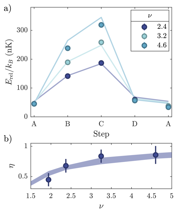
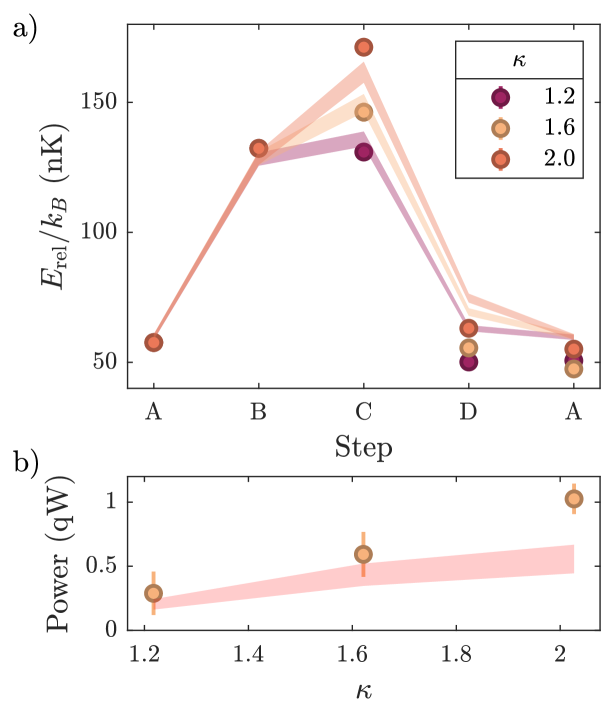
Fig. 2a shows close agreement between numerically calculated and experimentally measured release energies. This correspondence provides additional retroactive justification for the isentropic assumption, and also demonstrates that approximate analytic expressions describing only the condensate with particles provide relatively accurate estimates of the energy. The analytic formulas for release energy and total energy are [44]
| (7) |
and
| (8) |
with , the zero-temperature chemical potential, the reduced temperature, the critical temperature of a harmonically confined Bose gas, the Riemann zeta function, and the Boltzmann constant. These results are accurate to within about 3% of approximation-free numerical simulations at the measured condensate fraction. The numerical results shown in Fig. 2b do indicate that accounts for 10% to 15% of the total energy in steps through , violating to some extent the Thomas-Fermi approximation. Evaluating the ratios and using energies obtained from simulations shows that the former is 1% to 3% larger than predicted while the latter is 0.1% to 0.6% larger.
A natural parameter to tune in order to maximize efficiency is the compression ratio . Fig. 4a shows measured release energy evolution over one cycle for different values of . At higher compression ratios we observe distinctly higher release energies for steps and but no significant changes to the values at steps and , in agreement with expectations from Eqs. 7 and 8. Fig. 4b demonstrates that increasing the compression ratio increases the efficiency , which asymptotically approaches unity. In the Thomas-Fermi approximation this can be understood by analyzing the change in energy per particle [35]. Defining as the interaction ratio between steps and , the efficiency can be expressed as
| (9) |
As , and is independent of the interaction strength. This can be compared in loose analogy to the Otto cycle efficiency with the compression ratio and the specific heat ratio.
Similarly, we can isolate the effects of interaction strength ratio by holding the compression ratio constant. Following the same procedure used to derive Eq. 9, we find : the power is determined solely by the interaction ratio for a fixed compression ratio . Fig. 5a shows release energy evolution over one cycle for various interaction strength ratios corresponding to step interaction strengths of 120, 160 and 200, at a constant compression ratio and a particle number approximately 60% larger than in Fig. 2. Fig. 5b shows that the output power indeed increases with , with a departure from theoretical predictions at larger values of a possible hint of beyond-mean-field behavior. These results emphasize the importance of interaction effects in the engine: Feshbach tuning is the key parameter controlling energy transfer between magnetic and optical fields. This power enhancement is completely decoupled from the boost to efficiency achieved through stronger compression, and from the power enhancement due to decreased cycle time.
In conclusion, we have realized an isentropic thermodynamic engine with a quantum degenerate working fluid and demonstrated that it outperforms a classical counterpart. Experimental measurements of engine performance for various values of control parameters and degrees of adiabaticity are in good agreement with both low-temperature analytics and approximation-free numerical simulations. This work opens up a variety of interesting directions for future exploration. These include optimizing performance with shortcuts to adiabaticity [6, 12, 7, 39], realizing a quantum Otto refrigerator [45, 46, 47, 48, 49], applying similar techniques to quantum heat engines involving trapped reservoirs of hot and cold atoms, investigating the role of criticality [8], and experimentally exploring the effects of entanglement on quantum thermodynamic engines [50, 51, 52].
Acknowledgements.
We thank Kris Delaney and Ethan McGarrigle for theoretical contributions. D.W. acknowledges support from the National Science Foundation (2110584), the Air Force Office of Scientific Research (FA9550-20-1-0240), the Army Research Office (W911NF-20-1-0294), and the Eddleman Center for Quantum Innovation, and from the NSF QLCI program through grant number OMA-2016245. G.F. acknowledges support from NSF DMR-2104255 for the theoretical method development. R.S. and E.N.-M. acknowledge support from the UCSB NSF Quantum Foundry through the Q-AMASEi program (Grant No. DMR-1906325). Use was made of computational facilities purchased with funds from the National Science Foundation (CNS-1725797) and administered by the Center for Scientific Computing (CSC). The CSC is supported by the California NanoSystems Institute and the Materials Research Science and Engineering Center (MRSEC; NSF DMR 1720256) at UC Santa Barbara.Appendix A Numerical Simulations
To compose the full cycle in simulations, we must fix particle number, , cell volume, , and total entropy, , around the cycle. All experimental observables are calculated by averaging field operators as described in the main text. Operators for , internal energy [53] and Helmholtz free energy [54] have been derived previously. Release energy is calculated using the operator for internal energy derived in [53], excluding the contribution from the trap. Entropy is calculated from the Helmholtz free energy and internal energy. Note that this means is an output of the field theory, not a degree of freedom to be sampled, so the algorithmic cost is virtually independent of .
To perform the ensemble averaging, we allow the complex fields and to independently evolve in a fictitous complex Langevin (CL) dynamics scheme according to a set of coupled stochastic partial differential equations that generates a Markov chain of system configurations [42, 43]. Random noise correlations are chosen according to a fluctuation dissipation theorem [55, 56] that ensures that averages over CL time are equivalent to unbiased thermodynamic ensemble averages [57, 58], provided the CL dynamics have reached steady state prior to sampling. Although the operators may be complex, time or ensemble-average operators for physical observables are real.
We evolve the CL dynamics equations using the pseudospectral method detailed in [41], which decouples and to linear order for numerical stability, and gives near-linear scaling with real space and resolution. We converge spatial resolution and imaginary time resolution until finite size effects in and are no longer significant. For the simulations reported here, we use up to plane waves and 64 points in the direction. On an NVIDIA A100, the average simulation in continuous 3D space of approximately half a million particles at 170 nK converges to a time-independent solution in 2.5 hours, and by 24 hours statistical errors of the mean are less than 0.05% of the mean. The longest simulations reported in this study had a duration of approximately 49 hours.
We report only simulations computed with the average number of particles over the entire cycle. Initially, we performed two sets of simulations, one at and one at , to account for experimental error in measured particle number of the data in Fig. 2a. However, the range of simulation results was smaller than the line width in Fig. 2a. Relative uncertainty in experimental and is smaller than the relative uncertainty in , so we expect our results to be accurate for the reported experimental conditions. Cell volume is fixed such that the density distribution is well-contained within the simulation cell and finite size effects are no longer observed in the calculated release energy and entropy. For the largest sample, we used a simulation box of m. is constrained by first computing the entropy at step on the cycle using the experimental as an input parameter, then adjusting at all other points to maintain constant . Using this procedure, remains within 2.5% of its initial value in all cycles.
Appendix B Connection to the Otto Cycle
Here we draw an analogy between this isentropic thermodynamic cycle and the classical Otto cycle. First, following [59], we define a “harmonic volume” and write the total energy as
| (10) |
The “harmonic” pressure can then be derived using the fact that it is conjugate to volume:
| (11) |
or equivalently by substituting the Thomas-Fermi density into the integral of the harmonic pressure given in [59]. The harmonic volume and pressure are not merely formal analogies; the harmonic volume can be associated with the physical volume that the particles occupy and the harmonic pressure can be associated with the mechanical equilibrium of the system.
The total energy can then be rewritten as
| (12) |
and by using the definition of the Thomas-Fermi energy, we can recover an analogy to the ideal gas law:
| (13) |
It is important to note that while plays the role of an “effective temperature” it is unrelated to a thermal equilibrium. In our cycle, strokes of constant are analogous to isothermal strokes in the classical cycle.
We now have all of the pieces to establish a connection with the Otto cycle. The first stage is an adiabatic compression with compression ratio . This traces an adiabat in the -space.Using Eq. 13, the adiabat is defined by
| (14) |
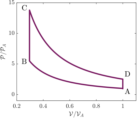
The heating stroke in the classical Otto cycle is replaced by an interaction strength stroke, which keeps the harmonic volume unchanged but changes the chemical potential and the harmonic pressure, thus mimicking an “isochoric” process. We note that this is not an actual transfer of heat, as the thermodynamic entropy is constant. The final two strokes follow the same arguments presented above. A quantitative diagram of this thermodynamic cycle is shown in Fig. 6.
This mathematical analogy enables an alternative derivation of the efficiency of the thermodynamic engine, allowing us to use the Otto cycle efficiency directly with the adiabatic exponent :
| (15) |
This is the same expression as Eq. 9 in the main text.
References
- Quan et al. [2007] H. T. Quan, Y.-x. Liu, C. P. Sun, and F. Nori, Phys. Rev. E 76, 031105 (2007).
- Zheng and Poletti [2014] Y. Zheng and D. Poletti, Phys. Rev. E 90, 012145 (2014).
- Zheng and Poletti [2015] Y. Zheng and D. Poletti, Phys. Rev. E 92, 012110 (2015).
- Kosloff and Rezek [2017] R. Kosloff and Y. Rezek, Entropy 19, 136 (2017).
- Hamedani Raja et al. [2021] S. Hamedani Raja, S. Maniscalco, G. S. Paraoanu, J. P. Pekola, and N. Lo Gullo, New J. Phys. 23, 033034 (2021).
- Beau et al. [2016] M. Beau, J. Jaramillo, and A. Del Campo, Entropy 18, 168 (2016).
- Li et al. [2018] J. Li, T. Fogarty, S. Campbell, X. Chen, and T. Busch, New J. of Phys. 20, 015005 (2018).
- Chen et al. [2019] Y.-Y. Chen, G. Watanabe, Y.-C. Yu, X.-W. Guan, and A. del Campo, npj Quantum Inf. 5, 1 (2019).
- Yunger Halpern et al. [2019] N. Yunger Halpern, C. D. White, S. Gopalakrishnan, and G. Refael, Phys. Rev. B 99, 024203 (2019).
- Barontini and Paternostro [2019] G. Barontini and M. Paternostro, New J. Phys. 21, 063019 (2019).
- Carollo et al. [2020] F. Carollo, K. Brandner, and I. Lesanovsky, Phys. Rev. Lett. 125, 240602 (2020).
- Keller et al. [2020] T. Keller, T. Fogarty, J. Li, and T. Busch, Phys. Rev. Research 2, 033335 (2020).
- Gluza et al. [2021] M. Gluza, J. a. Sabino, N. H. Y. Ng, G. Vitagliano, M. Pezzutto, Y. Omar, I. Mazets, M. Huber, J. Schmiedmayer, and J. Eisert, PRX Quantum 2, 030310 (2021).
- Boubakour et al. [2023] M. Boubakour, T. Fogarty, and T. Busch, Phys. Rev. Research 5, 013088 (2023).
- Eglinton et al. [2022] J. Eglinton, T. Pyharanta, K. Saito, and K. Brandner, arXiv.2212.12076 (2022).
- Myers et al. [2022] N. M. Myers, F. J. Peña, O. Negrete, P. Vargas, G. De Chiara, and S. Deffner, New J. Phys. 24, 025001 (2022).
- Roßnagel et al. [2014] J. Roßnagel, O. Abah, F. Schmidt-Kaler, K. Singer, and E. Lutz, Phys. Rev. Lett. 112, 030602 (2014).
- Zhang et al. [2014] K. Zhang, F. Bariani, and P. Meystre, Phys. Rev. Lett. 112, 150602 (2014).
- Park et al. [2019a] J.-M. Park, S. Lee, H.-M. Chun, and J. D. Noh, Phys. Rev. E 100, 012148 (2019a).
- Wu et al. [2006] F. Wu, L. Chen, F. Sun, C. Wu, F. Guo, and Q. Li, Energy Convers. and Manag. 47, 3008 (2006).
- Roßnagel et al. [2016] J. Roßnagel, S. T. Dawkins, K. N. Tolazzi, O. Abah, E. Lutz, F. Schmidt-Kaler, and Kilian Singer, Science 352, 325 (2016).
- Bu et al. [2023] J.T. Bu, J.Q. Zhang, G.Y. Ding, J.C. Li, J.W. Zhang, B. Wang, W.Q. Ding, W.F. Yuan, L. Chen, i. m. c. K. Özdemir, F. Zhou, H. Jing, and M. Feng, Phys. Rev. Lett. 130, 110402 (2023).
- Peterson et al. [2019] J. P. S. Peterson, T. B. Batalhão, M. Herrera, A. M. Souza, R. S. Sarthour, I. S. Oliveira, and R. M. Serra, Phys. Rev. Lett. 123, 240601 (2019).
- Brantut et al. [2013] J.-P. Brantut, C. Grenier, J. Meineke, D. Stadler, S. Krinner, C. Kollath, T. Esslinger, and A. Georges, Science 342, 713 (2013).
- Zou et al. [2017] Y. Zou, Y. Jiang, Y. Mei, X. Guo, and S. Du, Phys. Rev. Lett. 119, 050602 (2017).
- Nettersheim et al. [2022] J. Nettersheim, S. Burgardt, Q. Bouton, D. Adam, E. Lutz, and A. Widera, PRX Quantum 3, 040334 (2022).
- Klatzow et al. [2019] J. Klatzow, J. N. Becker, P. M. Ledingham, C. Weinzetl, K. T. Kaczmarek, D. J. Saunders, J. Nunn, I. A. Walmsley, R. Uzdin, and E. Poem, Phys. Rev. Lett. 122, 110601 (2019).
- Bouton et al. [2021] Q. Bouton, J. Nettersheim, S. Burgardt, D. Adam, E. Lutz, and A. Widera, Nat. Commun. 12, 2063 (2021).
- Koch et al. [2022] J. Koch, K. Menon, E. Cuestas, S. Barbosa, E. Lutz, T. Fogarty, T. Busch, and A. Widera, arXiv:2209.14202 (2022).
- Park et al. [2019b] J.-M. Park, S. Lee, H.-M. Chun, and J. D. Noh, Phys. Rev. E 100, 012148 (2019b).
- Watanabe et al. [2020] G. Watanabe, B. P. Venkatesh, P. Talkner, M.-J. Hwang, and A. del Campo, Phys. Rev. Lett. 124, 210603 (2020).
- Jaramillo et al. [2016] J. Jaramillo, M. Beau, and A. d. Campo, New J. Phys. 18, 075019 (2016).
- Hu et al. [2016] M.-G. Hu, M. J. Van de Graaff, D. Kedar, J. P. Corson, E. A. Cornell, and D. S. Jin, Phys. Rev. Lett. 117, 055301 (2016).
- Dalfovo et al. [1999] F. Dalfovo, S. Giorgini, L. P. Pitaevskii, and S. Stringari, Rev. Mod. Phys. 71, 463 (1999).
- Pethick and Smith [2008] C. Pethick and H. Smith, Bose-Einstein Condensation in Dilute Gases, 2nd ed. (Cambridge University Press, 2008).
- Zener [1932] C. Zener, Proc. R. Soc. A 137, 696 (1932).
- Stringari [1996] S. Stringari, Phys. Rev. Lett. 77, 2360 (1996).
- Brandner et al. [2015] K. Brandner, M. Bauer, M. T. Schmid, and U. Seifert, New J. Phys. 17, 065006 (2015).
- Schaff et al. [2011] J.-F. Schaff, X.-L. Song, P. Capuzzi, P. Vignolo, and G. Labeyrie, EPL 93, 23001 (2011).
- Negele and Orland [1998] J. W. Negele and H. Orland, Quantum Many-particle Systems (Advanced Book Classics) (Perseus Books, 1998).
- Delaney et al. [2020] K. T. Delaney, H. Orland, and G. H. Fredrickson, Phys. Rev. Lett. 124, 070601 (2020).
- Parisi [1983] G. Parisi, Phys. Lett. B 131, 393 (1983).
- Klauder [1983] J. R. Klauder, J. Phys. A (1983).
- Pitaevskii and Stringari [2016] L. Pitaevskii and S. Stringari, Bose-Einstein Condensation and Superfluidity (Oxford University Press, 2016).
- Hartmann et al. [2020] A. Hartmann, V. Mukherjee, G. B. Mbeng, W. Niedenzu, and W. Lechner, Quantum 4, 377 (2020).
- Niedenzu et al. [2019] W. Niedenzu, I. Mazets, G. Kurizki, and F. Jendrzejewski, Quantum 3, 155 (2019).
- Abah et al. [2020] O. Abah, M. Paternostro, and E. Lutz, Phys. Rev. Res. 2, 023120 (2020).
- Jiao et al. [2021] G. Jiao, Y. Xiao, J. He, Y. Ma, and J. Wang, New J. Phys. 23, 063075 (2021).
- Karimi and Pekola [2016] B. Karimi and J. P. Pekola, Phys. Rev. B 94, 184503 (2016).
- Ji-Zhou et al. [2012] H. Ji-Zhou, H. Xian, and Z. Jie, Chin. Phys. B 21, 050303 (2012).
- Zhang et al. [2007] T. Zhang, W.-T. Liu, P.-X. Chen, and C.-Z. Li, Phys. Rev. A 75, 062102 (2007).
- Zhao and Zhang [2017] L.-M. Zhao and G.-F. Zhang, Quantum Inf. Process. 16, 216 (2017).
- Fredrickson and Delaney [2023] G. H. Fredrickson and K. T. Delaney, Field-Theoretic Simulations in Soft Matter and Quantum Fluids (Oxford University Press, 2023).
- Fredrickson and Delaney [2022] G. H. Fredrickson and K. T. Delaney, Proc. Nat. Acad. Sci. 119, e2201804119 (2022).
- McQuarrie [1976] D. A. McQuarrie, Statistical Mechanics (Harper & Row, New York, 1976).
- Van Kampen [1981] N. G. Van Kampen, Stochastic Processes in Physics and Chemistry (North-Holland, New York, 1981).
- Gausterer and Lee [1993] H. Gausterer and S. Lee, J. Stat. Phys. 73, 147 (1993).
- Lee [1994] S. Lee, Nucl. Phys. B 413, 827 (1994).
- Romero-Rochín [2005] V. Romero-Rochín, Phys. Rev. Lett. 94, 130601 (2005).