Three-dimensional decaying magnetic field
belonging to Beltrami flow
Department of Systems Innovation Engineering,
Faculty of Science and Engineering, Iwate University,
4-3-5 Ueda, Morioka, Iwate 020-8551, Japan
Abstract
This study analysed a three-dimensional Taylor decaying vortex under an applied magnetic field as a benchmark test problem to verify the calculation method of an electromagnetic fluid flow and investigated the validity of the decaying magnetic field model. First, we observed the flow structure of a three-dimensional Taylor decaying vortex without an applied magnetic field. We investigated the changes in the error between the calculation result and the exact solution when the number of grid points and the Reynolds number varied and showed the effectiveness of the benchmark test. Next, we analysed a three-dimensional Taylor decaying vortex under an applied magnetic field and clarified the characteristics of the decaying magnetic field. When a magnetic field is applied, low magnetic pressure regions are connected in a mesh pattern, and the magnetic pressure distribution with a distorted cubic structure occurs to surround a high magnetic pressure region. In a stagnation region, the magnetic energy becomes low, and the magnetic flux line is similar to the streamline of the velocity field. High current densities occur in a grid pattern, and the magnetic flux lines swirl around the high current density region. The magnetic pressure and magnetic energy are high in the high current density region. When the Reynolds number and the magnetic Reynolds number vary, the decay trends of various energies agree well with the exact solution. The transition to turbulent flow occurs at a high Reynolds number, and the kinetic and total energies decrease rapidly. After the dissipation rate of kinetic energy becomes maximum, the vortex structure decays, and the flow field approaches a stationary state without magnetic fields. The three-dimensional Taylor decaying magnetic field belonging to the Beltrami flow is a valuable model for verifying the calculation method of electromagnetic fluid flows.
Keywords Navier–Stokes equations, Computational methods, Vortex dynamics, Magnetic fields, Turbulent transition
1 Introduction
Taylor (1923) derived an analytic solution for the two-dimensional flow field that satisfies the continuity equation and the Navier-Stokes equation. The solution represents a flow field in which the vortex decays, and the vortex is called a Taylor decaying vortex. This Taylor decaying vortex has been used to show the validity of a calculation method (Kim and Moin, 1985; Le and Moin, 1991; Jordan and Ragab, 1996). An exact solution representing a three-dimensional Taylor decaying vortex has also been proposed (Ross Ethier and Steinman, 1994; Barbato et al., 2007; Antuono, 2020).
Ross Ethier and Steinman (1994) derived an analytic solution for a three-dimensional decaying vortex using the method for deriving the solution for the two-dimensional Taylor decaying vortex. That solution is not periodic in the three directions of the coordinates, so it is necessary to model and give the boundary conditions. Barbato et al. (2007) found periodic solutions in the three directions using the method of Ross Ethier and Steinman (1994). In that solution, each velocity component does not contain all the spatial coordinates of the independent variable, so the solution does not represent a complete three-dimensional flow. Antuono (2020) proposed an analytic solution of a periodic three-dimensional flow in which all the velocity components depend on the coordinates in the three directions, using the method of Ross Ethier and Steinman (1994).
Discretization of the fundamental equation is significant for the stability of numerical calculation in unsteady flow with a high Reynolds number. The conservative difference scheme allows for stable calculations and conserves kinetic energy in inviscid fluids. Since energy transformation occurs in the flow of electromagnetic fluid, it is not easy to verify the energy conservation characteristics in numerical analysis. Assuming zero kinematic viscosity and magnetic diffusivity, each volume integral of total energy and cross-helicity is conserved in a periodic flow (Woltjer, 1958). Therefore, we can verify the conservation characteristics using these transport quantities for an inviscid periodic flow. It is hard to confirm whether energy is converted correctly in a viscous fluid. In addition, a difficult problem in an electromagnetic fluid analysis is to satisfy the constraint subjected to Gauss law for magnetism, that is, the condition of no divergence of magnetic flux density. When verifying a computational method for the flow of electromagnetic fluid, it is a suitable choice to use a model for which an analytic solution exists. Therefore, it is necessary to find an analytic solution for a three-dimensional flow under an applied magnetic field. If we can extend a mathematical model proposed by Antuono (2020) to a three-dimensional magnetic flow field, then we can use that model as a benchmark test. For a two-dimensional flow, Liu and Wang (2001) analysed the flow of the Taylor decaying vortex to which a magnetic field was applied.
In this study, we investigate a three-dimensional Taylor decaying vortex under an applied magnetic field and clarify whether that model is available for verifying the calculation method of an electromagnetic fluid flow.
2 Fundamental equation
The fundamental equations for the incompressible viscous flow of a Newtonian fluid under an applied magnetic field are the equations for mass, momentum, and magnetic flux density. The magnetic flux density must satisfy the constraint subjected to Gauss law for magnetism. These governing equations are given as
| (1) |
| (2) |
| (3) |
| (4) |
where is the time, is the fluid velocity vector at the coordinates , is the pressure, and and are the density and viscosity coefficient of the fluid, respectively. is the current density, is the magnetic flux density, and is the magnetic diffusivity. The term on the right side of the momentum conservation equation (2) represents the Lorentz force.
The current density is given using Ampere’s law as:
| (5) |
where is the magnetic permeability.
The above fundamental equations are nonlinear, and an analytic solution can be obtained only in a restricted case. We explain an analytic solution for a three-dimensional decaying vortex in the following.
3 Three-dimensional Taylor decaying vortex
3.1 Analytic solution without applied magnetic field
Antuono (2020) obtained a periodic three-dimensional analytic solution shown below using the method of Ross Ethier and Steinman (1994). Subscripts 1 and 2 represent two solutions.
| (6) | |||||
| (7) | |||||
| (8) | |||||
| (9) |
where . is the wavenumber and is the wavelength. The phase , , and are given as
| (10) |
| (11) |
where is a parameter, and the value excluding the singularity value is set. In this study, is set as in the existing study Antuono (2020). The two solutions show similar distributions. The variables in the fundamental equations are non-dimensionalized using the reference values of length , velocity , time , and pressure . The dimensionless exact solution is as follows:
| (12) | |||||
| (13) | |||||
| (14) | |||||
| (15) |
where is the non-dimensionalized wavenumber. The Reynolds number is defined as .
This flow of the three-dimensional Taylor decaying vortex belongs to the Beltrami flow. Therefore, the velocity vector and the vorticity vector are parallel, and . In addition, in the velocity and vorticity fields of this Beltrami flow, because the relationship of holds, the pressure is associated with the kinetic energy and enstrophy , respectively. Stagnation point is where the pressure is . Antuono (2020) clarified that the high-pressure region including the stagnation point has a Y-shaped structure. The stagnation point occurs at the next position.
| (16) |
where , , and are integers.
As in the two-dimensional case (Taylor, 1923), the three-dimensional Taylor decaying vortex flow is also periodic, so the volume integral of the velocity is zero. Since the total amount of pressure corresponds to the volume integral of kinetic energy, it is a constant value of for inviscid fluids. The volume-integrated kinetic energy is explained later.
| (17) |
where .
The kinetic energy is given as
| (18) |
The volume-integrated kinetic energy and the average kinetic energy are given as
| (19) |
| (20) |
The time when the average kinetic energy is halved is , and the time when decays to 10 % of the initial kinetic energy is .
3.2 Analytic solution under applied magnetic field
Assuming that the velocity vector and magnetic flux density vector represent the Beltrami flow, the exact solution of the velocity and pressure of the three-dimensional Taylor decaying vortex is expressed by the equation (15) even under an applied magnetic field. Using the three-dimensional Taylor decaying vortex model proposed by Antuono (2020), the magnetic flux density in an electromagnetic fluid under an applied magnetic field is given as
| (21) | |||||
| (22) | |||||
| (23) | |||||
The above equations satisfy the basic equations (3) and (4). As reference values dimensionless variables, the length is , velocity is , time is , pressure is , and magnetic density is . The exact solution is non-dimensionalized as follows:
| (24) | |||||
| (25) | |||||
| (26) | |||||
where is the non-dimensionalized wavenumber. The magnetic Reynolds number is defined as .
Since this three-dimensional magnetic flux density flow is the same as the Beltrami flow, the magnetic flux density vector and the current density vector are parallel, and . Therefore, the Lorentz force does not act, and work does not occur. Assuming that the kinematic viscosity and magnetic diffusivity are zero, the kinetic and magnetic energies are conserved in a periodic flow, and the total energy is also conserved. Therefore, it is useful to use this decaying vortex model as a benchmark test problem for verifying the validity of the energy conservation characteristics in a calculation method.
Since the flow of the three-dimensional Taylor decaying vortex is periodic, the volume integral of the magnetic flux density is zero like the velocity.
| (27) |
where .
The magnetic energy is given as
| (28) |
This magnetic energy corresponds to dimensionless magnetic pressure. The volume-integrated magnetic energy and the average magnetic energy are obtained as follows:
| (29) |
| (30) |
The total energy is . The volume-integrated total energy and the average total energy are obtained as follows:
| (31) |
| (32) |
Cross helicity is given as
| (33) |
The volume-integrated cross helicity and the average cross helicity are obtained as follows:
| (34) |
| (35) |
4 Numerical method and calculation conditions
4.1 Numerical method
For stable calculations, transport quantities such as kinetic energy must be conserved discretely in periodic flows of inviscid fluids. In addition, the analytical characteristics of the governing equation must hold discretely, and the compatibility between the conservative and non-conservative forms of convection term must be satisfied discretely. Similar to the previous research (Ham et al., 2002; Morinishi, 2009), we use the implicit midpoint law to discretize the time derivatives in the governing equations and perform time marching. The second-order central difference scheme is used for the discretization of the space derivatives. The simplified marker and cell method (Amsden and Harlow, 1970) is applied to solve the discretized equations. In this study, the Lorentz force is discretized using compact interpolation (Yanaoka, 2023), which can maintain the compatibility between conservative and non-conservative forms of the Lorentz force. We describe the Lorentz force discretization method in Appendix A.
4.2 Calculation conditions for three-dimensional Taylor decaying vortex
The calculation area is a cube with one side . A uniform grid of is used for the calculation. For error evaluation and grid dependency verification, we also use the grids with dimensions of , , and . Exact solutions and are given as initial conditions, and periodic boundary conditions are set as boundary conditions.
First, we verify the validity and stability of the present calculation method. To confirm whether non-physical kinetic energy is generated, we analyse the inviscid flow at . The calculation is performed up to the time under the condition that the Courant number is CFL=0.5.
Regarding the calculation conditions of the decaying vortex, the Reynolds numbers are , 50, , and . We calculate until the average kinetic energy is half and compare the calculation result with the exact solution. For each Reynolds number, the time step is given so that the Courant number CFL is constant regardless of the grid. The Courant number for Reynolds numbers other than is CFL=0.25. At , the time until the average kinetic energy is half is short, so the Courant number was set to CFL=0.05.
Similar to the earlier study (Antuono, 2020), this study performs a long-time calculation to confirm whether the transition to turbulent flow is observed. As in the previous study, the Reynolds number is . In this calculation, we also use a grid finer than the number of grid points used in the existing research. The Courant number is set to CFL=0.1 and 0.5 to verify the influence of time increments when the number of grid points is 41. In other grids, the Courant number is CFL=0.5. In addition, we investigate the effect of initial velocity disturbance on the flow transition. Similar to the previous study(Morinishi, 2009), we use the vector potential with uniform random numbers to generate an initial disturbance that satisfies the continuity equation. The disturbance levels are values corresponding to 1of the initial average kinetic energy. As an initial condition, we use the value obtained by adding this initial disturbance to the exact solution of velocity.
4.3 Calculation conditions for three-dimensional Taylor decaying vortex under applied magnetic field
Next, we consider the analysis of a three-dimensional Taylor decaying vortex under an applied magnetic field. The grids and boundary conditions used are similar to the analytical model described in the previous subsection. The exact solutions , , and are given as initial conditions.
Regarding the calculation conditions, the Reynolds numbers are set to and , referring to the existing research on two-dimensional Taylor decaying vortex (Liu and Wang, 2001; Yanaoka, 2023). The magnetic Reynolds numbers are and 50, and the Alfvén number is . We calculate under the condition that the Courant number CFL=0.25.
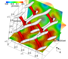
(a) velocity vectors, pressure contour, isosurface of pressure, and isosurface of 2nd invariant of velocity gradient tensor
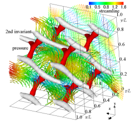
(b) velocity vectors, streamlines, isosurface of pressure, and isosurface of 2nd invariant of velocity gradient tensor
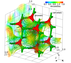
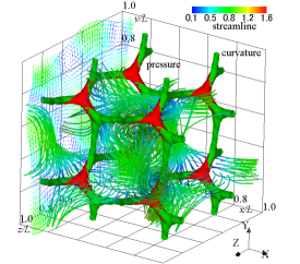
(c) velocity vectors, streamlines, isosurface of pressure, and isosurface of the curvature of equipressure surface
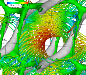
(d) streamlines, isosurface of 2nd invariant of velocity gradient tensor, and isosurface of the curvature of equipressure surface
4.4 Extraction of pressure structure
We explain the method of extracting low- or high-pressure regions. If pressure distribution is concentric around a vortex tube, we can identify the vortex tube by displaying the isosurface of the pressure. However, when the vortex tube and shear layer coexist, the pressure changes due to the two structures, so we cannot extract only the vortex tube. Because the radius of a thin vortex tube is small, we can identify the thin vortex tube by visualising a vortex tube with a large curvature. Therefore, by calculating the curvature of an equipressure surface and displaying the isosurface with a large curvature, we can identify a vortex tube with a small radius of curvature. Now we consider the case where pressure is high at the centre of a concentric circle and low at the periphery. The curvature of the pressure isosurface can be defined as follows:
| (36) |
where is a unit normal vector on the isosurface. Therefore, we can visualise a high-pressure region by displaying the high value of . Conversely, we can extract a low-pressure region by showing the low value of . is the radius of curvature of the vortex tube.
4.5 Characteristics of analytic solutions
Figure 1 shows the flow field of the analytic solution at . The velocity vectors, streamlines, and the contour and isosurface of pressure are shown. The second invariant of velocity gradient tensor and the curvature of an equipressure surface are also displayed in an isosurface form. The red isosurface of pressure shows the distribution of dimensionless pressure , and we can see the pressure field near a stagnation point. The second invariant of the velocity gradient tensor is a quantity that expresses the magnitude relationship between the strain rate tensor and the vorticity tensor. Structures with represent regions of high shear rates, where the high viscous dissipation rate of kinetic energy occurs. The second invariant of the velocity gradient tensor is a negative value of and represents a tubular high-shear region where the strain rate tensor increases. Along the direction of the vector , the tubular structure exists a little away from the stagnation point. The high-pressure region with the stagnation point is a Y-shaped structure (Antuono, 2020). To extract the structure of a high-pressure area near a stagnation point, we calculate the curvature of the isosurface of the pressure. The green isosurface represents its curvature, and the magnitude of the curvature is . The high-pressure regions, which indicate the low-velocity areas with stagnation points, are connected in a mesh pattern, and a distorted cube structure appears. We can see that the isosurface of curvature buries the isosurface of pressure, and the cube structure represents the structure of the pressure field. The pressure is low at the centre of this cube structure, and when looking at the streamline, a swirling flow occurs so as to go around the low-pressure region. The tubular high-shear structure passes through the high-pressure region, and the pressure at the centre of the tubular high-shear structure is higher than the central pressure of the decaying vortex. No clear rotational flow occurs around the tubular high-shear structure.
5 Results and discussion
5.1 Analysis of three-dimensional Taylor decaying vortex
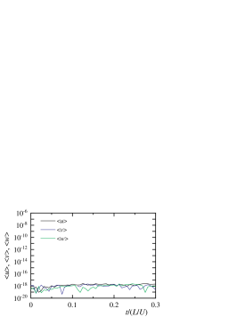
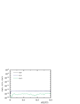
Figure 2 shows the time variation of the total amount of transport quantity in an inviscid analysis. , , and are the volume integrals of velocities of -, -, and -directions, respectively, and are the volume integral of kinetic energy. is the exact solution. Since the flow is periodic, each total amount of the transport quantity is preserved. The total amounts of the velocities change at the level of rounding error, indicating that the conservation characteristics of the present calculation method are excellent. In addition, the kinetic energy is kept constant and consistent with the exact solution, and no non-physical energy is generated. Therefore, since this calculation method has excellent stability and does not generate non-physical kinetic energy, it is considered that this method can simulate a decaying vortex in a viscous fluid without destroying its characteristics.
(a) velocity
(b) kinetic energy
(a) velocity vectors, pressure contour, isosurface of pressure, and isosurface of 2nd invariant of velocity gradient tensor
(b) velocity vectors, streamlines, isosurface of pressure, and isosurface of 2nd invariant of velocity gradient tensor
(c) velocity vectors, streamlines, isosurface of pressure, and isosurface of the curvature of equipressure surface
(d) streamlines, isosurface of 2nd invariant of velocity gradient tensor, and isosurface of the curvature of equipressure surface
Figure 3 shows the flow field of at time . The isosurface values were set so that the size of the structure represented by the isosurface was the same as the structure size shown in figure 1. The red isosurface expresses the distribution of the dimensionless pressure . The pressure near the stagnation point becomes lower than the initial value shown in figure 1. The second invariant of the velocity gradient tensor is , and we find that the tubular high-shear structure with the initial strength of diffuses and decays. Since the vorticity of the Taylor decaying vortex decreases with time, the magnitude of the strain rate tensor inside a high-shear structure generated by the interaction between vortices also decreases. The curvature of the pressure isosurface is , which is the same as the initial value. Over time, the cube structure in which the high-pressure regions are connected in a mesh pattern is maintained. The velocity of the swirling flow inside this cubic structure becomes slow.
(a) velocity

(b) kinetic energy
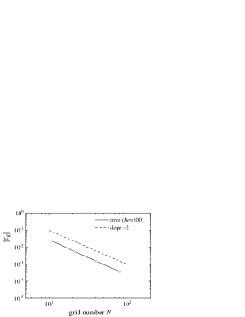
Figure 4 shows the time variations of the total amounts of velocities and kinetic energy at . The total amount of each velocity is the level of rounding error. The kinetic energy decays over time. This calculation results well agree with the exact solution, indicating that this calculation method accurately captures the characteristics of the decaying vortex. The three-dimensional periodic decaying vortex proposed by Antuono (2020) is an effective model for investigating the conservation characteristics of calculation methods and changes in kinetic energy.
(a) kinetic energy
(b) error

(a) without initial disturbance
(b) with initial disturbance
For , the relative error of kinetic energy at the time after the average kinetic energy is half is shown in figure 5. The error is defined as . This error also corresponds to the relative error of pressure. As the number of grid points increases, the error decreases with the slope of , indicating that the calculation is the second-order accuracy.
(a) velocity
(b) kinetic energy
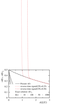
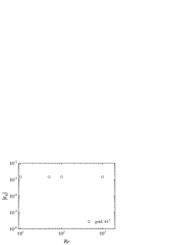
Figure 6 (a) shows the time variation of the total amount of kinetic energy at each Reynolds number. Regardless of , the time variation of kinetic energy well agrees with the exact solution. Also, as increases, the attenuation of kinetic energy slows down. Ham et al. (2002) performed a calculation in which the time progress was inverted in an inviscid periodic flow field and showed the reversibility of the calculation method. This study set a negative time step at and used the result of as an initial value. Then, the time marching was performed in the opposite direction. The result is plotted in the figure. Intriguingly, we can calculate the phenomenon that the decaying vortex returns to its original state even in the viscous fluid. It was possible to calculate until the time near . However, as time passed, the calculation diverged on the way, and the decaying vortex could not be completely restored to its original state. In the case of Courant number 0.25, it was possible to calculate up to near , but the calculation diverged on the way. Although this phenomenon is physically impossible, this time-reversal simulation may be an effective tool as a method for verifying the stability and conservation characteristics of a calculation method. Figure 6 (b) shows the relative error when the Reynolds number varies. The error maintains constant regardless of . Since we can confirm the calculation accuracy by changing the number of grid points and the Reynolds number, it is considered that the three-dimensional Taylor decaying vortex model is valuable as a benchmark test.
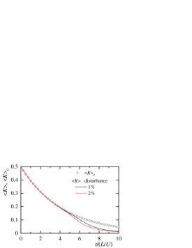
Next, for , the time variation of the kinetic energy up to the time is shown in figure 7 (a) using three grids. In the analysis using the number of grid points of , we varied the Courant number and investigated the influence of time increment. At , the kinetic energy sufficiently attenuates. In the case of the number of grid points , there is a slight difference between the calculation result and the analytic solution. On the other hand, the results obtained using finer grids well agree with the exact solution. Even if we perform the calculation over a long time, this calculated value well agrees with the exact solution, and there is no difference with time increments. In the previous study (Antuono, 2020), the difference between the calculation result and the analytic solution increased with time, and the transition to turbulent flow was observed. This study could not confirm such a transition phenomenon at . Figure 7 (b) shows the calculation result when an initial disturbance is added to the initial condition of the velocity. From around time , the difference between the calculation result and the exact solution occurs, and the same trend as the existing research (Antuono, 2020) appears. We can see that increasing the initial disturbance accelerates the transition. For investigating the transition phenomenon of a decaying vortex, the analysis of a decaying vortex with an initial disturbance is an intriguing investigation.
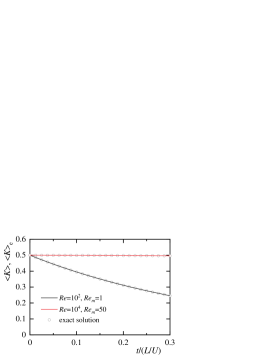
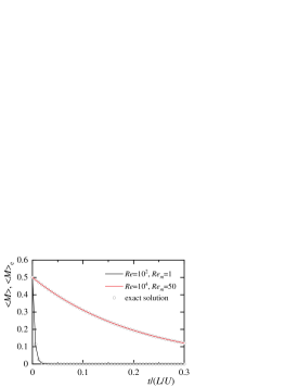
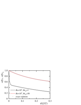
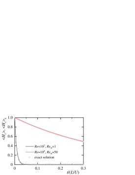
(a) magnetic flux density

(b) magnetic energy
(c) total energy
(d) cross helicity

(a) kinetic energy
(b) magnetic energy
(c) total energy
(d) cross helicity
5.2 Analysis of three-dimensional Taylor decaying vortex under applied magnetic field
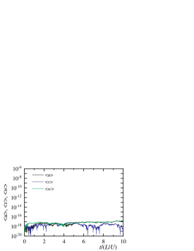
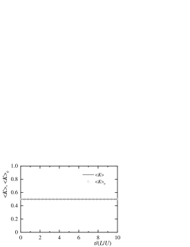
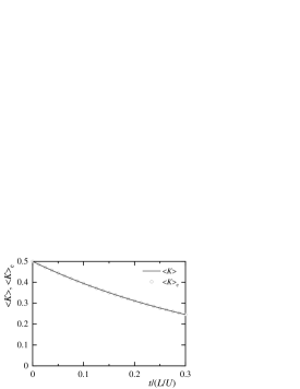
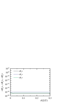
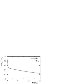
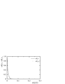
Figure 8 shows the time variations of the total amounts of velocities and kinetic energy at . In addition, figure 9 shows the time variations of the total amounts of magnetic flux density, magnetic energy, total energy, and cross helicity at . Since the magnetic flux density is periodic, the total amount is conserved and analytically zero. The total amount of calculated magnetic flux density is the level of rounding error. The kinetic and magnetic energies decay with time, and the magnetic energy decays sharply. Since no Lorentz force occurs, we can confirm from the comparison of figures 4 and 8 that the kinetic energy is consistent with the result with no applied magnetic field. If a non-physical Lorentz force occurs, the attenuation of kinetic energy is overestimated. The total energy and cross helicity agree well with each exact solution. Since the magnetic Reynolds number is low, the magnetic energy decays quickly, and most of the total energy at corresponds to the kinetic energy.
For , the relative error of the total energy at the time after the average kinetic energy is half is shown in figure 10. The error decreases with a slope of , indicating that the calculation method is the second-order accuracy.

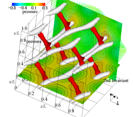
(a) magnetic flux densities in -, -, and -directions
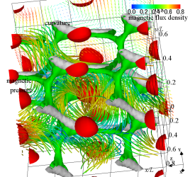
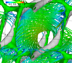
(b) magnetic flux density lines, and isosurfaces of magnetic pressure, 2nd invariant of velocity gradient tensor, and curvature of magnetic pressure isosurface
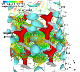
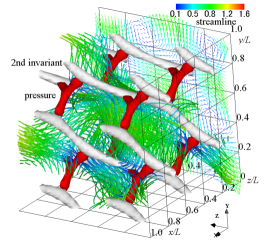
(c) magnetic flux density lines, and isosurfaces of magnetic pressure, current density magnitude, and 2nd invariant of velocity gradient tensor

(a) kinetic energy
(b) total energy
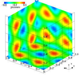
(a) initial pressure
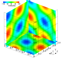
(b) initial vorticity
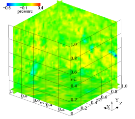
(c) pressure
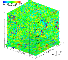
(d) vorticity
Next, we investigate the trend of the decaying vortex when the calculation conditions vary. Figure 11 shows the time variations in the kinetic, magnetic, and total energies and cross helicity at and . For comparison, the results of and are also included. This calculation result agrees well with the exact solution, and the present analysis can capture the energy decay process. Under and , there is almost no attenuation of the kinetic energy. On the other hand, the magnetic energy, total energy, and cross helicity decay over time.
Figure 12 (a) shows the distribution of the magnetic flux density at time . The -, -, and - cross-sections show the distribution of magnetic flux densities in the -, -, and -directions, respectively. At this time, the distinct periodicity of the magnetic flux density remains. In addition, figures 12 (b) and (c) show the magnetic flux lines, the magnetic pressure, the magnitude of the current density vector, the second invariant of the velocity gradient tensor, and the curvature of the isosurface of magnetic pressure. Here, we calculated the curvature of the isosurface of magnetic pressure to visualise the region of low magnetic pressure. The red isosurfaces show the distributions of magnetic pressure and , and the light blue isosurface expresses the current density magnitude , indicating the occurrence of high current density. The silver isosurface shows the second invariant of the velocity gradient tensor and represents a tubular high-shear region. The green isosurface shows the curvature of the magnetic pressure isosurface, and we can confirm the region of low magnetic pressure. The high magnetic pressure is shown in figure (b), and the low magnetic pressure and the magnitude of high current density are shown in figure (c). In figure (b), the magnetic pressure distribution of a distorted cubic structure appears so that the regions of low magnetic pressure are connected in a mesh pattern and surround the areas of high magnetic pressure. At this time, the attenuation of the velocity field is small, so the clear vortex structure is present. The magnetic flux density decays, but the magnetic flux lines are similar to the streamlines of the velocity field. The distribution of magnetic pressure shown in figure (c) is Y-shaped and the same as the shape of the pressure distribution in figure 3. The dimensionless magnetic pressure corresponds to the dimensionless magnetic energy. Therefore, the magnetic energy becomes high in the region, where the magnetic pressure is high. The high current density occurs in a grid pattern, and the magnetic flux lines swirl so as to surround the high current density region. In the area of high current density, the magnetic pressure, that is, the magnetic energy becomes high.
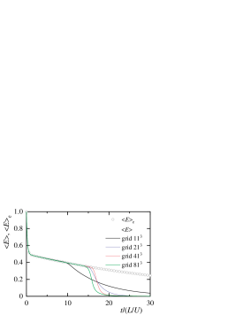
Figure 13 shows the time variations in the kinetic and total energies at and . Over time, the difference between the result obtained using each grid and the exact solution appears, and the kinetic and total energies decay sharply. An existing study (Antuono, 2020) reported that the difference from the analytic solution suggested a transition to turbulent flow. When the flow transition occurred, the magnetic energy had sufficiently decreased. Therefore, under this condition, the influence of the magnetic field on the flow transition is considered small. As the number of grid points increases, the transition points approach the dimensionless time .
The vorticity distribution at time and 16.85 is shown in figure 14. The -, -, and - cross-sections show the vorticity distributions in the -, -, and -directions, respectively. In the initial state, a large-scale vortex exists, but at , it can be seen from the figure that it is converted to small-scale vortex structures by a non-linear effect and attenuated.
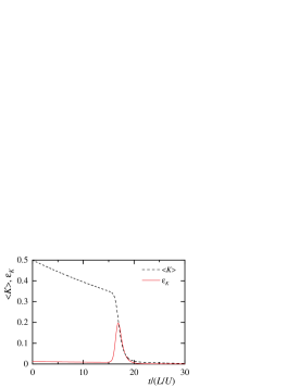
Figure 15 shows the time variation of the kinetic energy and its dissipation rate . The dissipation rate is defined as . As the kinetic energy decays sharply, the dissipation rate increases and a maximum value appears. The pressure and vorticity distributions when the dissipation rate is maximum were shown in figures 14 (c) and (d). The vortex structure disappears with time due to viscous dissipation, the induced magnetic field also disappears, and the flow field asymptotically approaches the stationary state.
6 Conclusions
In this study, we analysed a three-dimensional Taylor decaying vortex under an applied magnetic field and investigated the effectiveness of the decaying magnetic field model for verifying the calculation method of electromagnetic fluid flow. The following findings were obtained.
First, we investigated the characteristics of a three-dimensional Taylor decaying vortex without an applied magnetic field. In the flow field where the decaying vortex exists, high-pressure regions are connected in a mesh pattern so as to include stagnation points, and the pressure distribution with a distorted cubic structure appears around a low-pressure region. A tubular high-shear structure, which passes through the cube structure, exists, and a swirling flow forms around the low-pressure region inside the cube. Furthermore, we investigated the total amounts of velocity, pressure, and kinetic energy when the number of grid points and the Reynolds number varied and clarified the conservation characteristics of the transport quantities in the three-dimensional Taylor decaying vortex.
Next, we analysed a three-dimensional Taylor decaying vortex under an applied magnetic field and clarified the characteristics of the decaying magnetic field. When a magnetic field is applied, low magnetic pressure regions are connected in a mesh pattern, and the magnetic pressure distribution with a distorted cubic structure occurs to surround a high magnetic pressure region. In a stagnation region, the magnetic energy becomes low, and the magnetic flux line is similar to the streamline of the velocity field. High current densities occur in a grid pattern, and the magnetic flux lines swirl around the high current density region. The magnetic pressure and magnetic energy are high in the high current density region. When the Reynolds number and the magnetic Reynolds number vary, the decay trends of various energies agree well with the exact solution. The transition to turbulent flow occurs at a high Reynolds number, and the kinetic and total energies decrease rapidly. After the dissipation rate of kinetic energy becomes maximum, the vortex structure decays, and the flow field gradually approaches a stationary state without magnetic fields.
The three-dimensional decaying magnetic field belonging to the Beltrami flow is a simple model for investigating the energy conservation characteristics of a calculation method and is also an intriguing target for studying the transition to turbulent flow and energy dissipation. This model of the three-dimensional decaying magnetic field is considered valuable as one benchmark test.
Appendix A Discretization of the Lorentz force
This study uses a staggered grid (Amsden and Harlow, 1970). We denote the cell centre as . The magnetic flux densities, , , and , are defined at the cell interface , , and , respectively, as with the velocity field. The coordinate transformation is performed so that equation can be discretized on non-uniform grids. As an example, the Lorentz force in the -direction can be transformed as follows:
| (37) |
where is the Jacobian defined as . The Cartesian coordinate in the physical space is transformed into the computational space . and are interpolated values. The variable at grid point is defined as . The interpolation in the ()-direction for the variable is given as
| (38) |
In this study, the current densities, and , are not defined at the same definition points as the velocities in the - and -directions, respectively. , , and are defined at the midpoints of the cell edges, , , and , respectively. In this case, 2 surrounding magnetic flux densities are required to calculate . The 2 surrounding current densities , are required to calculate . A total of 3 surrounding is required. In this way, the Lorentz force can be obtained by compact interpolation. In addition, the charge conservation law is satisfied at the grid point . This method is the compact interpolation (Yanaoka, 2023).
The Lorentz force is rewritten using compact interpolation from the non-conservative to the conservative form. The compatibility between conservative and non-conservative forms is preserved in discretized equations for uniform grids and approximately for non-uniform grids. Therefore, even if the non-conservative Lorentz force is discretized, the momentum and kinetic energy are conserved in inviscid fluids.
Acknowledgements. This research did not receive any specific grant from funding agencies in the public, commercial, or not-for-profit sectors. We would like to express our gratitude to Associate Professor Yosuke Suenaga of Iwate University for his support of our laboratory. The authors wish to acknowledge the time and effort of everyone involved in this study.
Declaration of interests. The authors report no conflicts of interest.
Author ORCID.
H. Yanaoka https://orcid.org/0000-0002-4875-8174.
References
- Amsden and Harlow (1970) Amsden, A.A., Harlow, F.H., 1970. A simplified MAC technique for incompressible fluid flow calculations. J. Comput. Phys. 6, 322–325. doi:doi:https://doi.org/10.1016/0021-9991(70)90029-X.
- Antuono (2020) Antuono, M., 2020. Tri–periodic fully three–dimensional analytic solutions for the Navier–Stokes equations. J. Fluid Mech. 890, A23. doi:doi:https://doi.org/10.1017/jfm.2020.126.
- Barbato et al. (2007) Barbato, D., Berselli, L.C., Grisanti, C.R., 2007. Analytical and numerical results for the rational large eddy simulation model. J. Math. Fluid Mech. 9, 44–74. doi:doi:https://doi.org/10.1007/s00021-006-0191-0.
- Ham et al. (2002) Ham, F.E., Lien, F.S., Strong, A.B., 2002. A fully conservative second–order finite difference scheme for incompressible flow on nonuniform grids. J. Comput. Phys. 177, 117–133. doi:doi:https://doi.org/10.1006/jcph.2002.7006.
- Jordan and Ragab (1996) Jordan, S.A., Ragab, S.A., 1996. An efficient fractional–step technique for unsteady incompressible flows using a semi-staggered grid strategy. J. Comput. Phys. 127, 218–225. doi:doi:https://doi.org/10.1006/jcph.1996.0170.
- Kim and Moin (1985) Kim, J., Moin, P., 1985. Application of a fractional-step method to incompressible Navier–Stokes equations. J. Comput. Phys. 59, 308–323. doi:doi:https://doi.org/10.1016/0021-9991(85)90148-2.
- Le and Moin (1991) Le, H., Moin, P., 1991. An improvement of fractional-step methods for the incompressible Navier–Stokes equations. J. Comput. Phys. 92, 369–379. doi:doi:https://doi.org/10.1016/0021-9991(91)90215-7.
- Liu and Wang (2001) Liu, J.G., Wang, W.C., 2001. An energy-preserving MAC–Yee scheme for the incompressible MHD equation. J. Comput. Phys. 174, 12–37. doi:doi:https://doi.org/10.1006/jcph.2001.6772.
- Morinishi (2009) Morinishi, Y., 2009. Fully conservative finite difference scheme for low–Mach number unsteady compressible flow simulations. JSME, Ser. B 75, 2153–2162. doi:doi:https://doi.org/10.1299/kikaib.75.759_2153. (in Japanese).
- Ross Ethier and Steinman (1994) Ross Ethier, C., Steinman, D.A., 1994. Exact fully 3D Navier–Stokes solutions for benchmarking. Int. J. Numer. Methods Fluids 19, 369–375. doi:doi:https://doi.org/10.1002/fld.1650190502.
- Taylor (1923) Taylor, G.I., 1923. Lxxv. on the decay of vortices in a viscous fluid. Philos. Mag. 46, 671–674. doi:doi:https://doi.org/10.1080/14786442308634295.
- Woltjer (1958) Woltjer, L., 1958. On hydromagnetic equilibrium. PNAS 44, 833–841. doi:doi:https://doi.org/10.1073/pnas.44.9.833.
- Yanaoka (2023) Yanaoka, H., 2023. Influences of conservative and non-conservative lorentz forces on energy conservation properties for incompressible magnetohydrodynamic flows. J. Comput. Phys. (accepted).