Three-to-one internal resonances in coupled harmonic oscillators with cubic nonlinearity
Abstract
We investigate a general system of two coupled harmonic oscillators with cubic nonlinearity, a model relevant to various structural engineering applications. As a concrete example, we consider the case of two oscillators obtained from the reduction of the wave propagation equations representing a cellular hosting structure with 1-dof resonators in each cell. Without damping, the system is Hamiltonian, with the origin as an elliptic equilibrium characterized by two distinct linear frequencies. To understand the dynamics, it is crucial to derive explicit analytic formulae for the nonlinear frequencies as functions of the physical parameters involved. In the small amplitude regime (perturbative case), we provide the first-order nonlinear correction to the linear frequencies. While this analytic expression was already derived for non-resonant cases, it is novel in the context of resonant or nearly resonant scenarios. Specifically, we focus on the 3:1 resonance, the only resonance involved in the first-order correction. Utilizing the Hamiltonian structure, we employ Perturbation Theory methods to transform the system into Birkhoff Normal Form up to order four. This involves converting the system into action-angle variables (symplectically rescaled polar coordinates), where the truncated Hamiltonian at order four depends on the actions and, due to the resonance, on one “slow” angle. By constructing suitable nonlinear and not close-to-the-identity coordinate transformations, we identify new sets of symplectic action-angle variables. In these variables, the resulting system is integrable up to higher-order terms, meaning it does not depend on the angles, and the frequencies are obtained from the derivatives of the energy with respect to the actions. This construction is highly dependent on the physical parameters, necessitating a detailed case analysis of the phase portrait, revealing up to six topologically distinct behaviors. In each configuration, we describe the nonlinear normal modes (elliptic/hyperbolic periodic orbits, invariant tori) and their stable and unstable manifolds of the truncated Hamiltonian. As an application, we examine wave propagation in metamaterial honeycombs with periodically distributed nonlinear resonators, evaluating the nonlinear effects on the bandgap particularly in the presence of resonances.
Acknowledgments Project ECS 0000024 Rome Technopole, CUP B83C22002820006, National Recovery and Resilience Plan (NRRP) Mission 4 Component 2 Investment 1.5, funded by the European Union - NextGenerationEU.
Funder Project funded under the National Recovery and Resilience Plan (NRRP), Mission 4 Component 2 Investment 1.5 - Call for tender No. 3277 of 30 December 2021 of the Italian Ministry of University and Research funded by the European Union - NextGenerationEU.
1 Introduction
Let us briefly recall the model introduced in [SW23jsv]. Figure 1 shows schematic view of the orthotropic plate model with the periodically distributed spider-web resonators. Each multi-frequency resonator should be meant as the multi-mass-spring system resulting from the multi-dof modal reduction of the infinite-dimensional resonator (i.e., the spider webs with a central mass, here represented in the figure, for the sake of graphical clarity, by a single mass-spring system instead of a set of mass-spring systems). The modal reduction is performed via the Galerkin projection method employing a number of mode shapes of the distributed-parameter resonators. Each resonator is represented by equivalent modal masses and modal springs.

The adopted plate theory (see [W]) with the elastic constants of the equivalent, homogenized orthotropic material describes the motion of the honeycomb with the attached resonators. By the Floquet-Bloch Theorem, which states that the solutions of the corresponding linear periodic resonators-plate system are quasi-periodic in space with the fundamental periodicity provided by the lattice period, the plate equation of motion can be projected onto the unit cell domain (i.e., the periodically repeated lattice unit). Then one obtains a system of coupled second order ODEs, being the number of retained resonators modes. For the metamaterial lattice with an array of equally spaced single-dof resonators, i.e., N = 1, equations reduce to the following system of second order ODEs
| (1) |
where and denote the nondimensional plate deflection and resonator relative motion at the origin of the fixed frame;
| (2) |
and
| (3) |
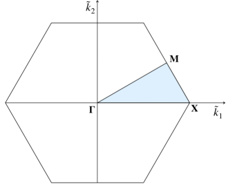
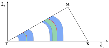
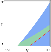
are the nondimensional modal mass and stiffness as functions of the nondimensional wave numbers , which stay within the irreducible Brillouin triangle (see Figure 2):
moreover
are the nondimensional plate bending stiffness coefficients; finally is the nondimensional nonlinearity.
Actually we consider the more general system of ODEs
| (4) |
where are unknown scalar functions, are real coefficients, is a symmetric positive definite real matrix and is a diagonal positive definite real matrix.
The existing literature on Hamiltonian and dissipative systems covers various topics, including bifurcations, invariant manifolds, and homoclinic and heteroclinic orbits. In [Fontich23], the authors study a one-parameter family of 2-DOF Hamiltonian systems with an equilibrium point undergoing a Hamiltonian-Hopf bifurcation. They focus on invariant manifolds and the behavior of the splitting of 2D invariant manifolds in the presence of homoclinic orbits. Similarly, [Celletti13] presents a KAM theory for conformally symplectic dissipative systems, demonstrating that solutions with a fixed n-dimensional (Diophantine) frequency can be found by an a-posteriori approach adjusting the parameters.
In [Llave06], the authors develop numerical algorithms to compute invariant manifolds in quasi-periodically forced systems, focusing on invariant tori and their asymptotic invariant manifolds (whiskers). These algorithms utilize Newton’s method and power-matching expansions of parameterizations. [Cabre05] describes a method to establish the existence and regularity of invariant manifolds, simplifying the proof of the stable manifold theorem near hyperbolic points by using the implicit function theorem in Banach spaces.
[H16] proposes a unified approach to nonlinear modal analysis in dissipative oscillatory systems. This approach defines nonlinear normal modes (NNMs) and spectral submanifolds, emphasizing the importance of damping for accurate conclusions about them, and the reduced-order models they produce. Lastly, [HW95], [HW96] and [HW93] develop methods to detect orbits asymptotic to slow manifolds in perturbed Hamiltonian systems, revealing complex chaotic behaviors and the creation of homoclinic orbits in resonant Hamiltonian systems through geometric singular perturbation theory and Melnikov-type methods.
1.1 Main results
We are interested here in small
amplitude solutions
of (4). In the first
approximation the system is linear
with linear frequencies
and
and the nonlinearity is a third order
perturbation.
If the linear frequencies
are non vanishing, distinct
and satisfy the non resonance
condition
the system can be integrated,
for instance, using the multiple scales method,
up to a smaller fifth order nonlinear remainder, see [SW23jsv].
In particular, [SW23jsv] provides explicit expressions for the nonlinear frequencies
of the truncated system (obtained
by disregarding the fifth order perturbation)
as functions of the
initial amplitudes. Moreover
the effects on the bandgap
were explored.
In [DL],
we analytically estimated the applicability threshold of the perturbative argument,
specifically the maximal admissible amplitude for which the above formula
is valid.
It was found that this applicability threshold decays to zero in the presence of resonances,
more precisely when the ratio between the optical and acoustic frequencies is
close to 3; indeed the 3:1 resonance is the only involved resonance
in the first order correction.
The methodology used is based on techniques from Hamiltonian Perturbation Theory.
Since the system is conservative,
we study it as a Hamiltonian
system. The origin is an elliptic
equilibrium and we put the
system in (complete) Birkhoff Normal Form
up to order 4 (3 in the equations
of motion).
The Birkhoff Normal Form
is a powerful tool in Hamiltonian
Perturbation Theory
that, through a suitable symplectic,
close-to-the-identity
nonlinear change of coordinates,
simplifies the Hamiltonian. More precisely, after introducing
action-angle variables111Essentially rescaled polar coordinates.,
in the non resonant case,
the truncated system at order four
is integrated, meaning
its Hamiltonian depends
only on the actions,
which are constant of motion,
and not on the angles.
As a consequence the phase space of the truncated Hamiltonian
is completely foliated by
nonlinear normal modes (NNMs), which are
two dimensional invariant tori filled with
periodic/quasi-periodic orbits
depending on whether the frequency ratio is rational/irrational.
Moreover such tori are (constant) graphs over the angles.
Finally the nonlinear frequencies
of the truncated Hamiltonian
are easily evaluated
as the derivatives of the Hamiltonian,
i.e. the energy, with respect
to the two actions.
This procedure, being perturbative in nature,
only works in a ball of small radius
around the origin. More precisely in [DL] we proved that there exists a constant , which
was explicitly estimated as function of the physical parameters, such that the smallness condition
reads
| (6) |
In contrast, the main aim of the present paper is to investigate what happens in the complementary regime, namely when the linear frequencies are in, or almost in, 3:1 resonance, specifically when
| (7) |
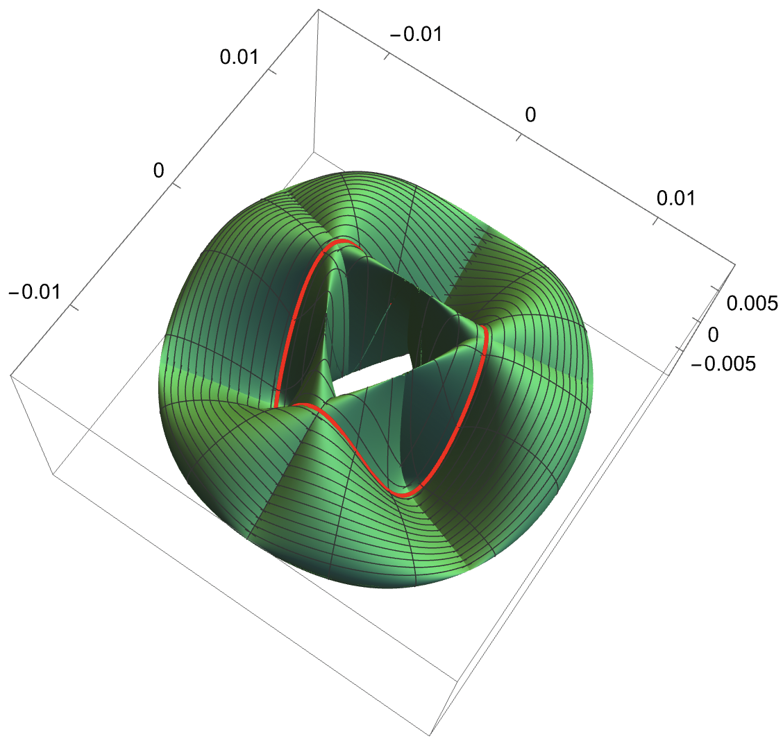
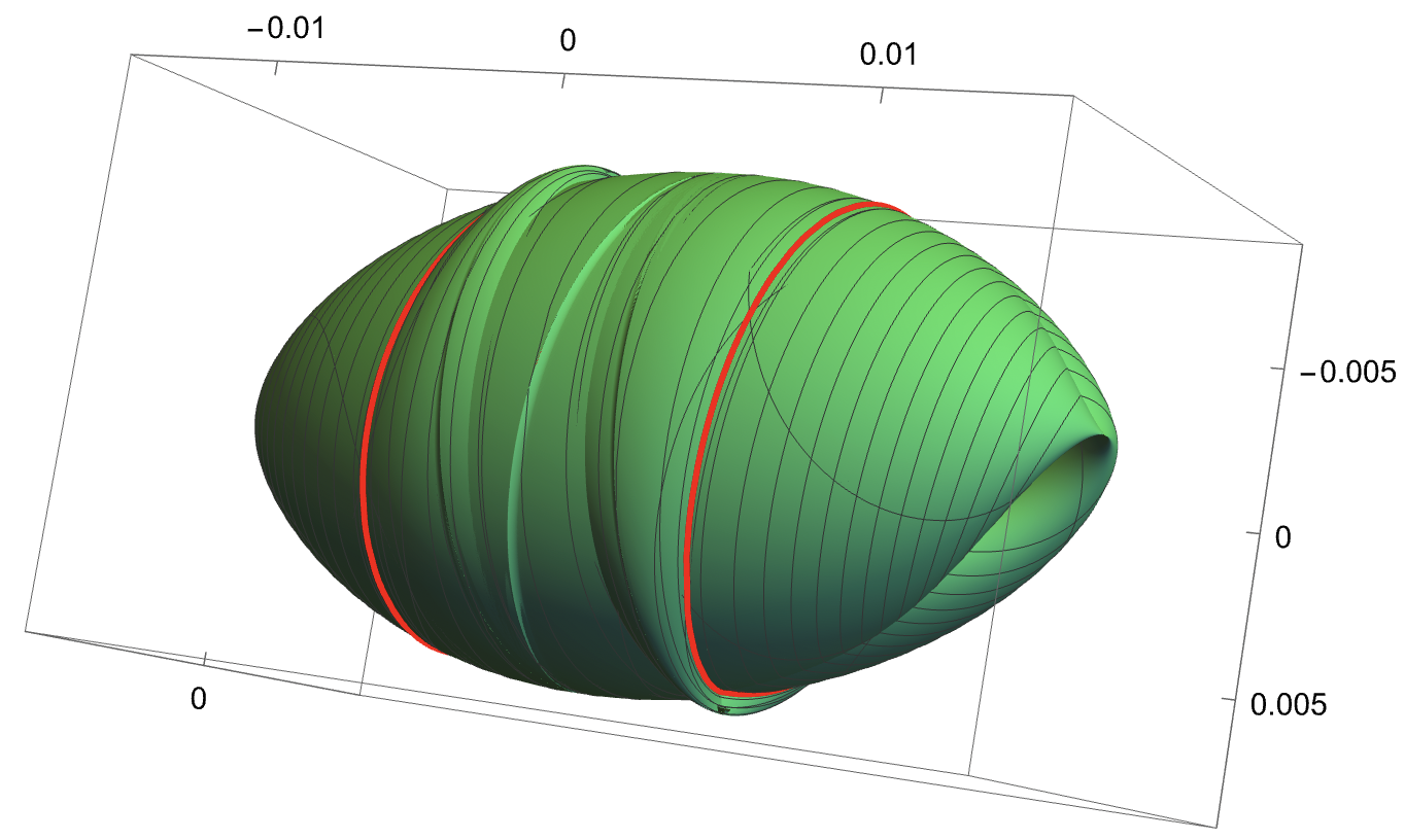
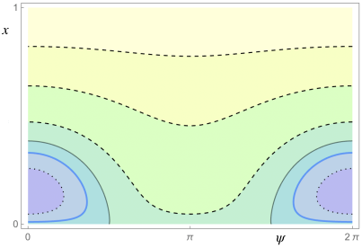
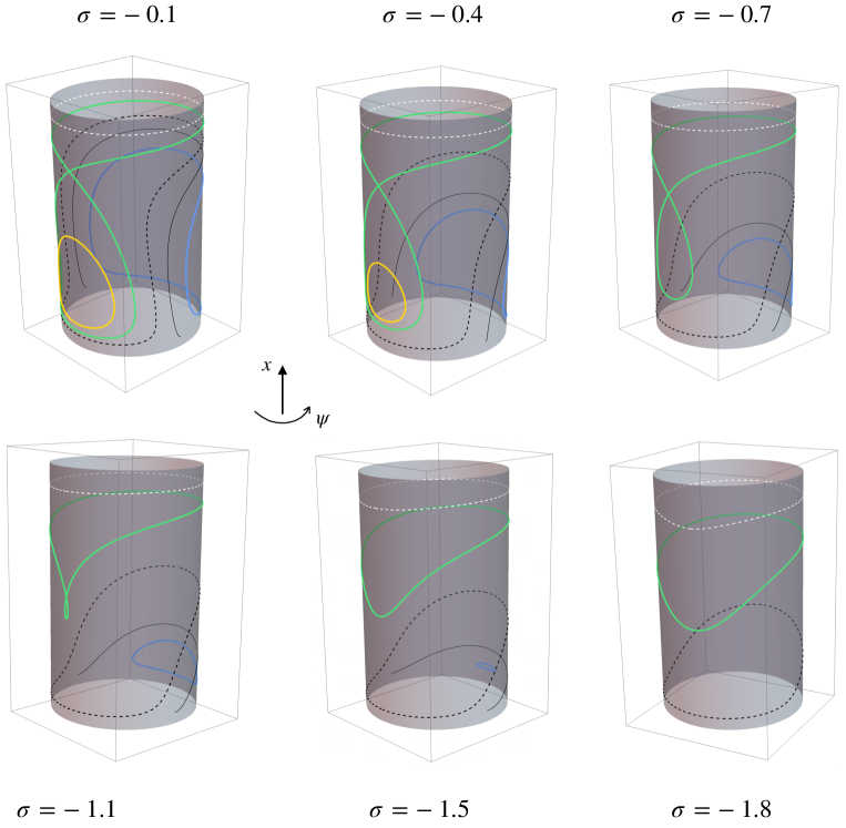
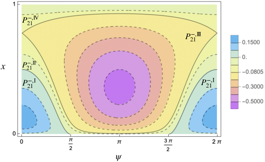
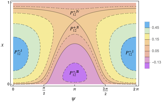
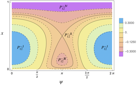
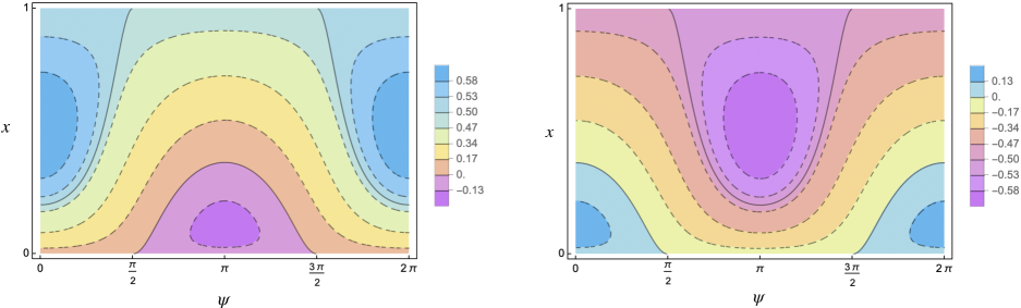
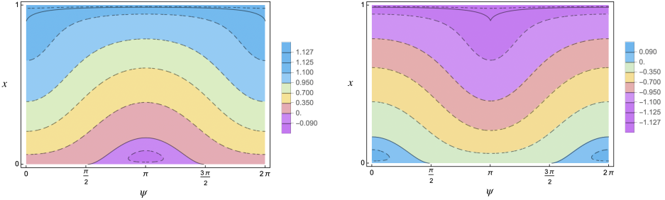
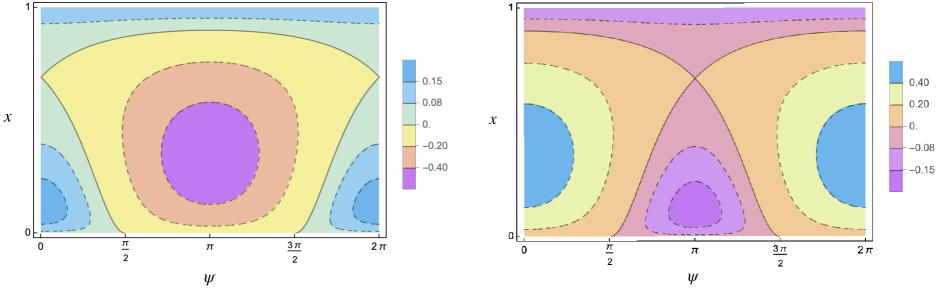
and is small enough. In this case, only a resonant BNF is available. This means that, after introducing action-angle variables and a linear symplectic change of coordinates, the truncated Hamiltonian at order four, (see (38)), depends on the actions and on one “slow” angle (as its associated frequency is small). The phase portrait becomes more complicated and interesting; its topology strongly depends on the values of the physical parameters. The phase space is still foliated by two dimensional NNMs (invariant tori) but many of them are no longer graphs over the angles as in the nonresonant case, exhibiting different topologies. Moreover, one dimensional NNMs appear such as: elliptic periodic orbits or even hyperbolic ones with their two dimensional (coinciding) stable and unstable manifolds. As the parameters vary, six possible topologically different phase portraits appear. An example is given in Figure 3.
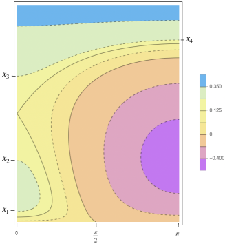
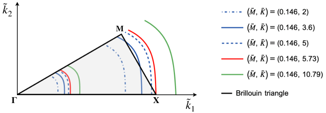
Let us denote by the action conjugated to the other angle, the “fast” one, which does not appear in . Then is a constant of motion for . For every fixed value of , evaluated at in the reduced bidimensional phase space containing only the slow angle and its conjugated action is a 1-degree-of-freedom Hamiltonian system. In this reduced system, the above two dimensional NNMs (invariant tori) correspond to one dimensional NNMs (periodic orbits), one dimensional NNMs (elliptic/hyperbolic periodic orbits) correspond to zero dimensional NNMs (elliptic/hyperbolic fixed points) and, finally, two dimensional (coinciding) stable and unstable manifolds correspond to one dimensional (coinciding) stable and unstable separatrices, respectively. Some examples are shown in Figures 3, 4 and 5.
Up to the singular222We call it singular since it is formed by all the points whose energy is singular, namely corresponds to some critical value of the Hamiltonian. set formed by the union of zero dimensional NNMs (equilibria) and one dimensional separatrices, the phase space of the reduced Hamiltonian is separated into two or four333According to the different values of the parameters. In Figure 3 a case with four regions is shown. open connected components having different topologies. Since the reduced system has one degree of freedom, on such connected components one can introduce suitable new action-angle coordinates, integrating the system. Recollecting, in these new variables, depends only on the new actions and the nonlinear frequencies are simply obtained as the derivatives of the Hamiltonian with respect to the actions.
However, we note that, at this stage, the nonlinear frequencies take the form of elliptic integrals, which are not simple to explicitly evaluate since both the integrating functions and the domains strongly depend on parameters. Nevertheless, we calculate them by using suitable Moebius transformations.
Finally, having the explicit formulas available, we study the nonlinear bandgap in the resonant regime. We found that, while the nonlinearity far from resonances can significantly change the bandgap, in the resonant case, the effect of resonances results in a less pronounced variation in the bandgap.
Here we study in details the truncated Hamiltonian giving a very precise description of its phase space and explicitly integrating the system. The case of the complete Hamiltonian is different since the system is genuinely two dimensional and, therefore, not integrable444Since the fast angle appears at higher order terms and, therefore, its conjugated action is not more a constant of motion.. However, using methods of KAM Theory one can prove the persistence of hyperbolic periodic orbits with their (local) stable and unstable manifolds as well as of the majority of invariant tori. Indeed, our analysis can bee seen as a necessary preparatory step toward applying KAM techniques in the resonant zones (see Remark 9).
Finally, we stress that our analysis is not limited to the case of the honeycomb metamaterials but applies directly to a wide range of problems modeled by two harmonic oscillators coupled with cubic nonlinearity as in equation (4).
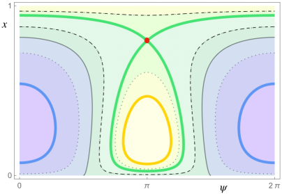
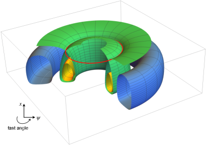
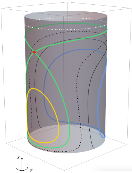
(Left bottom) A representation of the phase space of the truncated Hamiltonian , once we have fixed the constant of motion . The image is obtained by rotating the picture on the top by the fast angle from to . In particular, by rotation, the blue and yellow curves become two dimensional NNMs (invariant tori) and the red point and the green curve become, respectively, a one dimensional NNM (a hyperbolic periodic orbit) and its two dimensional (coinciding) stable and unstable manifolds.
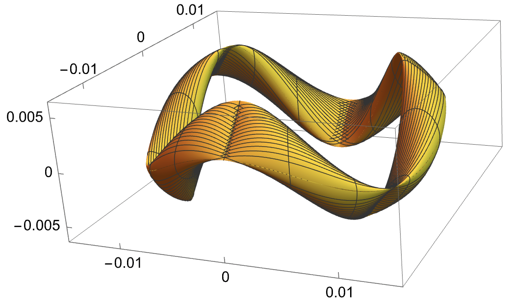
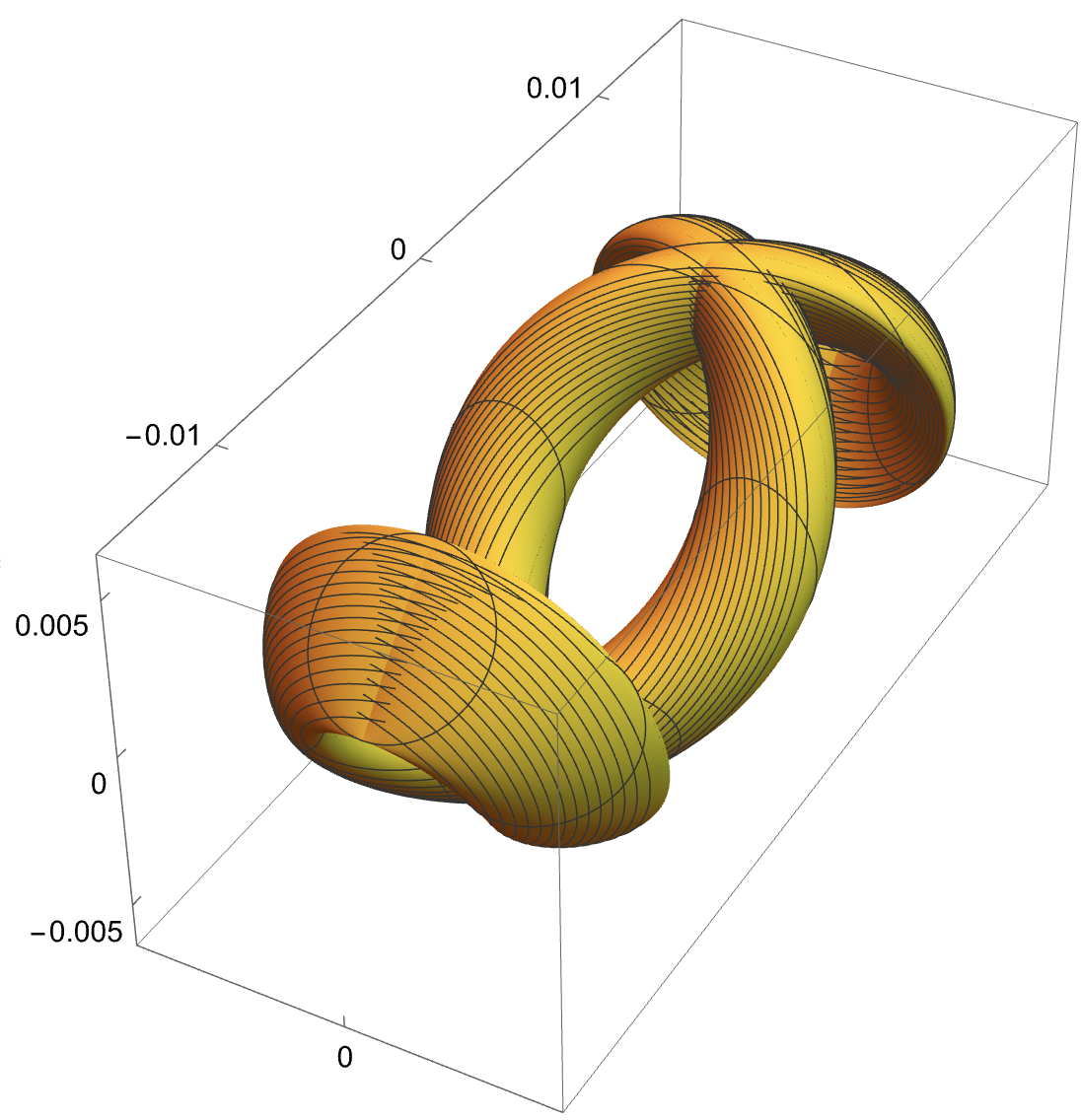
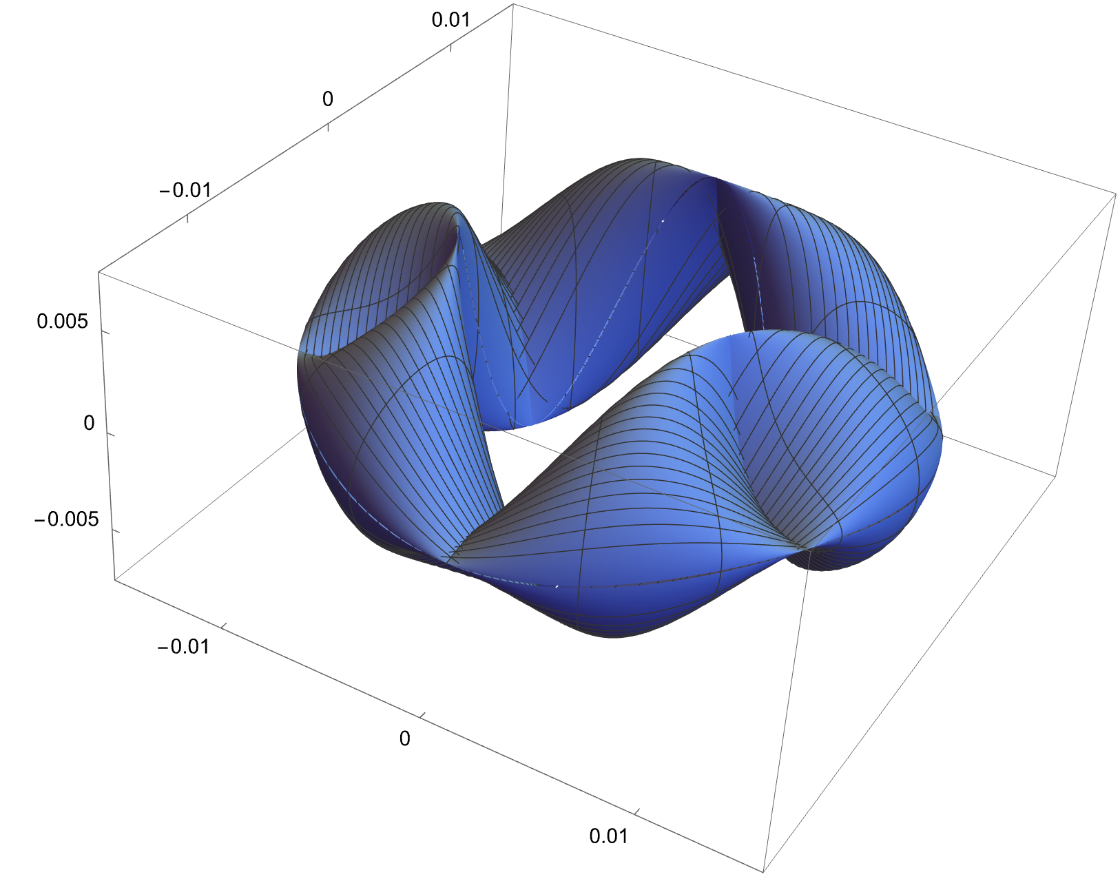
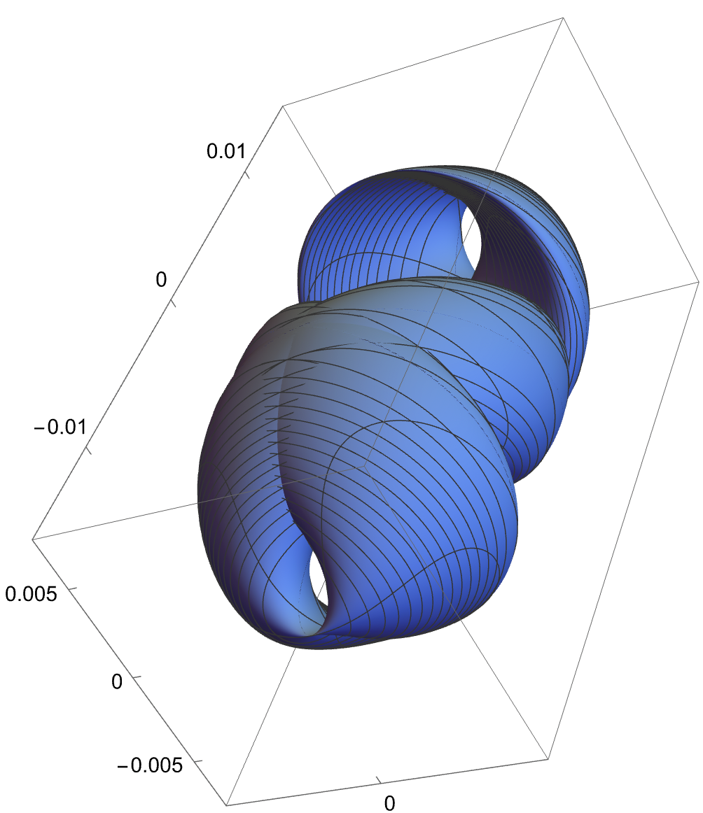
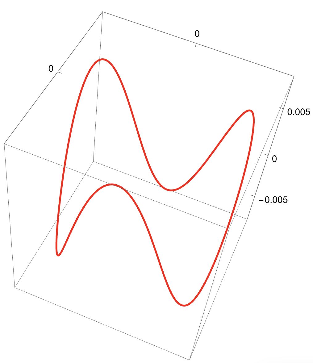
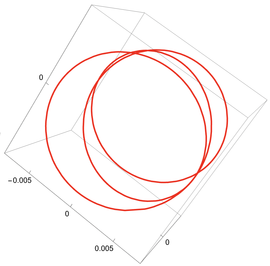
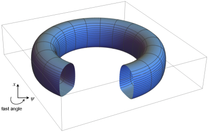
(Left bottom) A representation of the phase space of the truncated Hamiltonian , once we have fixed the constant of motion . The image is obtained by rotating the picture on the left by the fast angle from to . In particular, by rotation, the blue and yellow curves become two dimensional NNMs (invariant tori) and the red point and the green curve become, respectively, a one dimensional NNM (a hyperbolic periodic orbit) and its two dimensional (coinciding) stable and unstable manifolds.
1.2 Summary of the paper
Section 2: the resonant Birkhoff Normal Form
We reinterpret the problem as a Hamiltonian system (see (11)). In Subsection 2.1, we put the system, close to the origin, in resonant BNF. Then, we examine the Hamiltonian truncated at fourth order, which is equivalent to third order in the equations of motion, as it captures the essential characteristics of the overall motion. Upon introducing action-angle variables it becomes evident that the truncated, or “effective”, Hamiltonian, after a suitable linear change of variables (see (36)), also depends on one angle, known as the “slow” angle (see (38)), as its associated frequency is small or even zero on the exact resonance.
After a suitable rescaling, the effective Hamiltonian, depending on the slow angle and on the non-dimensional action , takes the form , where and depend on the physical parameters and on the other action (which is a constant of motion); see Subsection 2.2.
Section 3: the six possible phase portraits
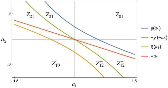
The behavior of the system depends on the number and on the nature of the critical points of , which, in turn, depends on the values of and . The gradient of can vanish only on the lines , when , or , when . At this point studying the solutions of these equations, as and vary, is crucial (see Figure 9). This identifies six zones in the plane , as detailed in Proposition 1, Lemma 5 and Figure 15. Correspondingly we have six possible configurations. When reached, the maximum of is attained on the line , conversely the minimum is attained on the line . E.g. let us briefly describe the scenario . By studying we have three possible cases: no critical points, a maximum and a minimum with negative energy, a maximum and a minimum with positive energy. On the other hand has a minimum. Note that the maximum of corresponds to a maximum for , the minimum of corresponds to a saddle for and the minimum of corresponds to a minimum of . Analogously, the complementary case gives rise to three additional configurations.
Section 4: construction of the integrating action variable
Since the action conjugated to the “fast” angle is a constant of motion, the truncated system has two independent conserved quantities (the other one is the energy) and, therefore, is integrable (by the Arnold-Liouville Theorem), in the sense that one can find a new set of symplectic action-angle variables in which the new Hamiltonian depends only on the actions. Although the theoretical construction of the integrating action is classic, finding an explicit analytical expression as a function of all the physical parameters involved is rather complicated.
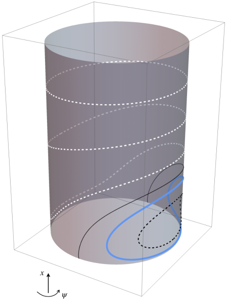
For every value of the energy , the new integrating action is given by the area enclosed by the level curve divided by , see Section 4. Such level curves are closed and can either wrap around the cylinder or remain confined to its surface without wrapping around it; see Figures 3 and 6.
Since is even in we can restrict to consider . In this set the level curves are graphs over and the area enclosed by them can be computed by an integral over , whose endpoints are the -coordinate of their intersections with the lines and . It turns out that these correspond to the roots , with , of the quartic polynomial , see (55) and Figure 25. As the energy varies, it is necessary to distinguish whether has or real roots555Note that, excluding the degenerate case of multiple roots, the number of real roots is even. and whether a root corresponds to an intersection with or . Explicit formulae for the roots are given in Subsection 3.5, see Figure 14.
Once we have defined the integrating action as a function of (and of the “dumb” action, let us say, ), the resulting integrated Hamiltonian will be its inverse . The nonlinear frequencies are given by the derivatives of the energy with respect to the actions, see (100), expressed through integrals, see Proposition 2. Such integrals are evaluated by suitable Moebius transformations in terms of elliptic functions, see Subsections 4.3 and 4.4.
Section 5: evaluation of the nonlinear bandgap for the honeycomb metamaterial
Finally, having the explicit formulas for the nonlinear frequencies available, we discuss the nonlinear bandgap for the honeycomb metamaterial, especially in the resonant regime. We found that, while nonlinear effects far from resonances can significantly alter the bandgap, in the resonant case the nonlinear frequencies, especially the acoustic one, closely align with the linear frequencies, resulting in a less pronounced variation in the bandgap.
2 The Hamiltonian structure and resonant BNF
In this section, after introducing optical and acoustic modes, we identify the system in (4) as Hamiltonian, see (11) below, and we evaluate the coefficients of the Hamiltonian, see (22). Set
where are the positive eigenvalues of and . Since is symmetric and is diagonal, there exists a matrix such that
| (8) |
where is the identity matrix. Consider the change of variables
| (9) |
By Lemma 8 the system in (4) is transformed into
| (10) |
In particular
Introducing the momenta , the system in (10) is Hamiltonian with Hamiltonian
| (11) |
where
| (12) |
Indeed it is immediate to see that the Hamilton’s equations , are equivalent to the system in (10). Since is a homogeneous polynomial of degree we write
| (13) |
Introducing coordinates , through
| (14) |
we have that the Hamiltonian in the new variables reads
| (15) |
In complex coordinates, ,
| (16) |
the Hamiltonian reads
| (17) |
where
| (18) |
Note that in complex coordinates the Hamilton’s equations of motion are
| (19) |
In the following we use the multi-index notation
| (20) |
for suitable coefficients with (analogously for ). In these notation, recalling (13) and (18), we rewrite as666Where, for integer vectors we set .
| (21) |
where
| (22) |
Note that .
2.1 Resonant BNF
The aim of the BNF is to construct a symplectic change of variables that “simplifies” the Hamiltonian in (17). First note that a Hamiltonian depending only on and writes and is integrable; in particular and are constants of motion. In light of the above considerations we guess if it is possible to find, in a sufficiently small neighborhood of the origin
| (23) |
a close-to-the-identity symplectic transformation that “integrates” up to terms of degree 6 in , which are smaller. This amounts to transform into , with
| (24) |
where, recalling (22),
| (25) |
As well known, this is possible if the nonresonance condition is satisfied for every couple of integers with and is small enough. It is simple to show (see, e.g. Proposition 1 in [DL]) that
While, by hypothesis, , (introduced in (6)) could be zero or small. It turns out that there exists a constant (see [DL] for a proof and the evaluation of ) such that, if
| (26) |
then it is possible to construct a symplectic transformation putting in (complete) BNF up to order 4, namely . Otherwise, if is too small with respect to777In particular we can assume that . , namely if , but still satisfies a suitable (weaker888With .) smallness condition , only a resonant BNF is available. This means that, in the case
| (27) |
through a symplectic transformation, the Hamiltonian takes the form , where
| (28) |
Remark 1.
The construction of the above symplectic transformation in the resonant case was given in [DL], where the remainder was explicitly estimated. This means that we found a concrete constant depending on the parameters such that .
Remark 2.
We now introduce action-angle variables999, . through the transformation
| (29) |
Remark 3.
Note that the above map is singular at or and is defined for .
In the symplectic variables in (29) the truncated Hamiltonians and take the final forms
| (30) | |||||
| (31) | |||||
| (32) |
The frequencies of the integrable nonresonant truncated Hamiltonian in (31) are the derivatives of the energy with respect to the actions, namely, by (32),
In particular, when , by (25) we have
| (33) |
where are the initial amplitudes. Note that in the original variables and , one has
| (34) |
that correspond, by (14), (16) and (29), in initial action-angle variables:
| (35) |
Formula (2.1) was already known (see [SW23jsv] or [DL]), but it does not hold close to resonances. To obtain the analogous of formula (2.1) in the resonant case is much more complicated since one has to integrate the Hamiltonian in (30). This is exactly what we are going to do in the following sections. The analogous of (2.1) in the resonant case are the formula (153)-(156) below.
Remark 4 (Reversibility).
Since the Hamiltonian in (30) is even in the system is reversible, namely if is a solution the same holds true for . In particular if the solution is even in the actions and odd in the angles, namely and .
2.2 The slow angle and the effective Hamiltonian
It is convenient to introduce the adimensional effective Hamiltonian depending solely on one angle , namely the “slow angle”. Let us consider the canonical transformation
so that
| (36) |
Note that has integer entries and so that the inverse has also integer entries. This implies that and its inverse are well defined on the torus . Note also that, by (29), we have
| (37) |
Let us write in (30) in the -variables
| (38) |
where
| (39) |
Note that is reversible in the sense of Remark 4. Moreover it depends only on the “slow angle” , that evolves by a small frequency (recall (7)), but does not depend on the “fast angle” , that, on the contrary, evolves by a frequency , which is definitively different from zero. So the partial derivative w.r.t. of vanishes and, by the Hamilton’s equations, , so that is a constant of motion, namely
Moreover the fast angle simply evolves as . It remains to study the evolution of the variables.
Being a constant of motion the dynamic of the “resonant truncated Hamiltonian” in (38) is simply generated by the one-degree-of-freedom “effective Hamiltonian”
| (40) |
with defined in (39). At this point it is convenient to introduce the “adimensional Hamiltonian”101010Also is adimensional.
| (41) |
and rewrite as a function of the “adimensional action”
| (42) |
by (37). We have the following
Lemma 1.
It results that
| (43) |
where
| (44) |
Remark 5.
Note that depends on only through , which depends on only through . Moreover at the exact resonance the dependence on disappears.
Since does not appear in , the conjugated action is a constant of motion and is actually a one degree of freedom Hamiltonian system depending on as a parameter. From now on we consider the one degree of freedom Hamiltonian on the phase space with .
3 The phase portrait
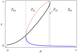
In this section we study the phase portrait of the adimensional Hamiltonian in (41) describing level curves, critical points and extrema. An important remark, that simplifies the treatment, is the fact that, thanks to (43), has, up to the rescalings and , the same level curves, critical points and extrema as the auxiliary function in (1). Such objects are studied in Subsections 3.1, 3.2 and 3.3, respectively. As usual, the new action coordinates, that integrate the system, are defined as the areas enclosed by the level curves. In order to evaluate them its important to determine the intersections between the level curves and the lines and since they appear as endpoints of the involved integrals. It turns out that such intersections correspond to the real roots of the quartic polynomial , see (55) and Figure 25. As the energy varies, it is necessary to distinguish whether has or real roots111111Note that, excluding the degenerate case of multiple roots, the number of real roots is even. and whether a root corresponds to an intersection with or . Explicit formulae for the roots are given in Subsection 3.5, see Figure 14. In Subsections 3.6 and 3.7 as the parameters vary, six topologically different scenarios appear.
3.1 Critical points, elliptic and hyperbolic zones
We now describe how the critical point of depends on the values of the parameters and in (1). First we note that is a critical point of if and only if is a critical point of the auxiliary function defined on (recall (1)). Moreover the nature of a critical point (maximum, minimum or saddle) is the same for and . Then in the following we will study critical points of as the parameters and vary.
It is immediate to see that, since
and , the critical points of have the form with or with . Namely
| (45) | |||||
| (46) |
where
| (47) |
The number of solutions of equations (45),(46) depends on the parameters .
Set
| (48) |
and121212Note that .
| (49) |
In particular the following result holds
Proposition 1.
If then has critical points and critical points. More precisely:
-
•
If then has a positive maximum at some and is strictly decreasing;
-
•
If then has a negative minimum at some and is strictly increasing;
-
•
If then has a positive maximum at some , while has a negative minimum at some and a maximum at some , with ;
-
•
If then has a positive maximum at some and a minimum at some , with , while has a negative minimum at some .
As a corollary, if then has critical points of the form and critical points of the form . More precisely:
-
•
If then has a positive maximum at ;
-
•
If then has a negative minimum at ;
-
•
If then has a positive maximum at , a negative minimum at and a saddle at ;
-
•
If then has a positive maximum at , a saddle at and a negative minimum at .
proof. See Appendix.
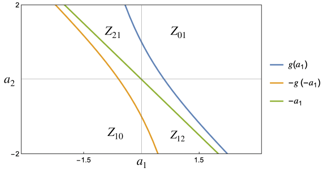
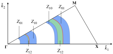
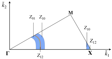
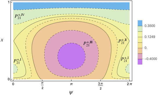
We call , hyperbolic zones, since they contain hyperbolic equilibria, and , elliptic zones, since they contain only elliptic equilibria. For any fixed pair , it is possible to identify which wave numbers in the Brillouin triangle give rise to resonant normal forms with different phase portraits. In particular if the corresponding values of and belong to , , then the phase portrait contains one hyperbolic and two elliptic equilibria, while, for and belonging to , only elliptic equilibria appear (see Figure 11). For brevity we denote by BNF of type the corresponding Birkhoff Normal Form.

Remark 6.
3.2 Extrema
We now discuss the extrema of in (1) and their dependence on the parameters . Following the notation of Proposition 1 we set
| (50) |
Then define
| (51) |
Since for every , , , we have that
Note that
since and for small enough since and . Note that in the cases we have , since the function has only one critical point (a maximum); analogously in the cases we have , since the function has only one critical point (a minimum). Moreover in the case ; indeed the function has no critical points then , moreover is increasing close to zero since . Analogously in the case . Finally in the case we have , since the function has a maximum at and a saddle at with . Analogously in the case we have .
3.3 Level curves
Since is even with respect to we can reduce to consider the “half phase space” . Take an energy with , and consider the level set . If , namely , since is not a critical point (being and recalling Proposition 1 and (3.2)), we can locally131313Namely in a sufficiently small neighborood of . express as a curve by the implicit function theorem. In particular, in the half phase space , we can always express as a function of , indeed the equation has the unique solution
| (52) |
Since the domain of definition of the is , the domain of is
We now discuss the structure of . Consider first the case in which 0 is an accumulation point for ; then it must be . Indeed, taking the limit for , in the inequality , we get . Moreover, when ,
| (53) |
Claim 1.
1 cannot be an accumulation point for , since we are assuming that (recall Remark 6).
proof. Indeed assume, by contradiction, that 1 is an accumulation point for . Then taking the limit for , , in the inequality we get . Substituting in the above inequality and dividing by we get
Taking again the limit for we get , which contradicts the assumption .
As a consequence, assuming , we have that is a compact set contained in ; moreover it is not difficult to see that it is formed by a finite number of closed intervals (possibly isolated points), whose endpoints satisfy one of the equations
| (54) |
This amounts to find the roots of the quartic polynomial
| (55) |
with .
Lemma 2.
If is not a critical energy for141414Namely the energy of a critical point of . , the roots of the quartic polynomial in (55) with are simple.
proof. By contradiction, if is a multiple root of , then . Write
Assume that , the case being analogous. By it follows that
| (56) |
Since and , by (56) we get . This means that is a critical point of , which is a contradiction since is a not critical energy.
From now on we will assume that is not a critical energy of . We denote the roots of with by with . We label the roots in increasing order, namely .
3.4 The quartic equation
In studying the solutions of (54) (equivalently of (55)) on , it is convenient to consider the real variable and make the substitution
Since
and
the two equations in (54) are equivalent to
| (57) |
Lemma 3.
proof. If for some , then satisfies (57) and, therefore (54), with the plus sign. As a consequence . The proof in the case is analogous.
When the polynomial reduces to , whose two roots are easily evaluated. Then we can reduce to the case and consider the equivalent monic polynomial , namely
| (60) |
The above quartic polynomial is called “depressed” since it is monic and its third order coefficient vanishes. Obviously and have the same roots. An immediate corollary of Lemma 3 is the following
Lemma 4.
Remark 7.
If has four real distinct roots and (so that is not a root), then the number of positive/negative roots depends on the sign of defined in (60). Indeed, since , the number of positive/negative roots is even if and odd otherwise.
3.5 Finding the roots of the quartic equation
Following [CP23] we find the roots of the quartic polynomial in (60). First set151515Compare formulas (20) and (10) in [CP23].
Let us define the positive161616Compare Theorem 8 in [CP23]. number as
| (61) |
Then the roots of are given by171717Compare formula (9) in [CP23].
| (62) |
The number of real roots of is:
4 if ,
2 if ,
0 if .
Let us now define
| (63) |
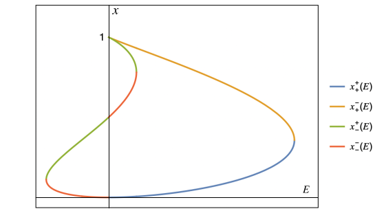
Note that is an increasing function of . By Lemma 4 are the roots of in (55). We now want to order the real roots in increasing order . We have different cases (see Figure 14):
| (67) | |||||
| (71) | |||||
| (72) |
3.6 The separatrices at the saddle points
Recall the definition of the zones
given in (49).
We now consider the curve with zero energy
bifurcating from the point (recall (53))
in the “half phase space”
.
In the case
such curve “turns left”
and touches the line at some point
.
Analogously
in the case
such curve “turns right”
and touches the line at some point
.
The situation in the cases and is more
involved; more precisely
it depends on the sign of .
In particular for we set
| (73) |
so that
The next result characterises the sets in (73)
Lemma 5.
Setting
| (74) |
we have
| (75) |
Note that, since is odd and for , by the definition of and it follows that and .
proof. We discuss only the case , the study of being analogous. As we said above, the picture of the phase space in the case strongly depends on the sign of the energy of the saddle point , where is the minimum of the function . In particular we claim that if and only if . In particular we note that satisfies the system
By algebraic manipulation we get
by which we finally have
By using (47)
| (76) |
Note that . By inverting the first expression in (76) we get ; substituting in the second expression we obtain that defined in (74). Therefore in , namely when , the value of the function at its minimum is exactly 0. On the other hand in , namely when , one has . Finally in it is .
3.7 Different topologies of the level curves
Let us consider the energy level sets in the phase spase
which is a cylinder. The points where the level curves touch the lines or are the solutions of the equation and , respectively; equivalently they are the roots of the quartic polynomial in (54).
We note that in the cases , the set has only one connected component. The same holds in the case except for when possesses two connected components. Analogously in the case the level set possesses two connected component for and only one otherwise.
Remark 8.
Up to the energy level corresponding to
and to the critical energies181818Namely the energy
of critical points of .
In the case
, that we are actually excluding (recall Remark 6),
there is also a curve which
touches the line ., the level sets are curves
of three types:
(i) a homotopically trivial, namely contractible,
curve making a loop around the maximum
intersecting twice the line ;
(ii) a curve wrapping on the cylinder; in particular it intersects once the line and once the line ;
(iii) a homotopically trivial
curve making a loop around the minimum
intersecting twice the line .
In the following we will always label the roots of the quartic polynomial in (54) so that . Recall Proposition 1.
Case .
The zero level separatrix actually separates the phase space into two open connected components and supporting two different kind of motions191919Where .
| (77) |
with . Indeed in the level curves have the form in case (ii) above, while in they have the form in case (i). In the present case the quartic polynomial in (54) possesses, for and not critical, only two real roots . Note that and . If the –level curve starts at and come back on the line at , otherwise, for , it joints the line at and the line at . Recalling (52), the level curve can be expressed as a graph over by the function .
Case .
We set
| (78) |
with . Again the zero level separatrix actually separates the two different kind of motions: in the level curves have the form in case (iii) above, while in they have the form in case (ii).
Case .
The zero level separatrix and the two separatrices emanating from the saddle point with energy202020Recall Proposition 1 and (3.2). (recall (73)) separate the phase space into 4 open connected components:
| (79) | |||
with . The level curves in and have the form case (ii) above, the ones in have the form in case (i), finally the ones in are as in (iii). In particular the level curves in pass through the points and ; the ones in through and ; the ones in through and ; the ones in through and .
Case .
The zero level separatrix and the two separatrices emanating from the saddle point with energy (recall (73)) separate the phase space into 4 open connected components:
| (80) |
while and are the two open connected components of with containing in its closure. We immediately see that
The level curves in and have the form in case (ii) above, the ones in have the form in case (i), finally the ones in are as in (iii). In particular the level curves in pass through the points and ; the ones in through and ; the ones in through and ; the ones in through and .
Case .
The zero level separatrix and the two separatrices emanating from the saddle point with energy (recall (73)) separate the phase space into 4 open connected components:
| (81) |
while and are the two open connected components of with containing in its closure. We note that
The level curves in and have the form case (ii) above, the ones in have the form in case (i), finally the ones in are as in (iii). In particular the level curves in pass through the points and ; the ones in through and ; the ones in through and ; the ones in through and .
Case .
The zero level separatrix and the two separatrices emanating from the saddle point with energy (recall (73)) separate the phase space into 4 open connected components:
| (82) |
with . The level curves in and have the form in case (ii) above, the ones in have the form in case (i), finally the ones in are as in (iii). In particular the level curves in pass through the points and ; the ones in through and ; the ones in through and ; the ones in through and .
3.8 Degenerate cases
Recalling Remark 6, we briefly illustrate in Figures 22-24 the degenerate cases: , when is a solution of (45)-(46), and , when two solutions coincide, finally , when the separatrix and the stable and unstable manifolds of the saddle point coincide and have zero energy.
4 Explicit formulae of the nonlinear frequencies
In this section we first write the integrating action as a function of the energy in terms of integrals in the variables with endpoints given by the roots of the quartic polynomial in (55), studied in the previous section. In addition to energy, these representation formulae depend on the values of the parameters and , according to the resulting different topologies of the phase space described above.
The final integrated Hamiltonian is the inverse of the function in (88). Its derivatives with respect to and are the nonlinear frequencies and can be written in terms of the derivatives of with respect to and , see (95). These derivatives are expressed in terms of elliptic integrals in Proposition 2. The integrals are explicitly evaluated by means of suitable Moebius transformations in Subsections 4.3 and 4.4, in the case that has four or two real roots, respectively. In the last subsection we consider the exact 3:1 resonance case, where the above formulae simplify a bit.
4.1 Construction of the integrating action variables
Since has two independent integrals of motions: the Hamiltonian itself and , by the Arnold-Liouville theorem the Hamiltonian is integrable. A part from the construction of the other action as function of the energy is as follows. is simply the area enclosed by the level curves of divided by . Such level curves coincide with the ones of .
Our aim is to find a symplectic map , fixing
| (83) |
such that, in the new coordinates, the Hamiltonian is integrated, namely212121Recalling (41) note that is adimensional.
| (84) |
depends only on the new actions .
Note that the same transformation also integrates in (41) and in (38). Indeed
| (85) |
In the new coordinates, the actions are constants of motion and the angles perform a linear motion with frequencies
| (86) |
The classical construction of the Hamiltonian , “the adimensional energy”, is as follows. First one constructs, for every fixed value of , the action function defined as the area enclosed by the level curve normalised by . Then, since the function turns out to be monotone (being ), one defines as its inverse. Namely, in view of (43),
| (87) |
So the level curves of play a crucial role here. Note that by (41) the level curves of
are the same as the ones of ,
moreover by (43) they are simple related
to the ones of .
More precisely the new action is defined as222222Recall (43).
| (88) |
where, recalling the notation introduced in
Remark 8, is the area (normalised by )
enclosed by the -level curve in the cases (i) and (iii),
and below the level curve
in the case (ii).
In particular we have four cases indexed by
,
according if one is in the zones
.
Case . The level curve makes a loop around the maximum
then232323Recall (52).
| (89) |
This holds in the zones:
Case .
The level curve wraps on the cylinder
| (90) |
in the cases .
Case .
The level curve makes a loop around the minimum
| (91) |
This holds in the zones: .
Case . The level curve wraps on the cylinder
| (92) |
in the cases .
Remark 9 (KAM Theory).
The above integrating construction holds
for the truncated Hamiltonian in (38)
but it does not work for
the complete Hamiltonian.
In fact
the complete system is genuinely two dimensional
and, therefore, not integrable. In particular
is not more a constant of motion.
One might wonder whether, for small enough, the invariant structures, both NNMs and stable and unstable manifolds, that exist for the truncated Hamiltonian survive, slightly deformed, for the full Hamiltonian. The answer is substantially positive
thanks to KAM Theory.
More precisely, the hyperbolic periodic orbit and its (local) stable and
unstable manifolds survive
as can be demonstrated following, e.g.,
[Graff] and [Val].
The conservation of two dimensional invariant tori
is ensured when the frequencies are strongly rationally independent. This implies that the majority of invariant tori
still exist in the complete system, whereas
a minority is destroyed.
However we note that, in this resonant case,
the application of KAM Theory is not straightforward.
In fact the standard KAM theory only regards
the persistence of the so called primary tori,
namely tori that are graphs over the angles.
However, as we have already shown, in the
resonant case also the so called secondary tori
appear (the blue and the yellow tori in Figure 5).
All our analysis can bee seen as a
necessary
preparatory
step in view of the application of
KAM techniques, since it integrates the
resonant BNF up to order four. This means that,
in the final action angle variables, the invariant tori
are graphs over the angles
and KAM methods can be applied.
For a KAM result in presence of resonances
and the persistence of secondary tori see
[MNT].
Finally we note that, since the complete system is, in general,
not integrable, KAM tori do not completely fill the phase space
but some gaps appear between them. In these gaps chaotic
behaviour may occur. However one has to notice that, since we
are in two degrees of freedom, every orbit is perpetually stable
in the sense that the solutions exist for all times
and the values of the action variables remain close to the initial ones
forever. The argument is standard in KAM Theory:
the orbits evolve on the three dimensional energy surface
we have two cases. 1) If on orbit starts on a KAM torus,
then it remains on it forever, since the torus is invariant for the
Hamiltonian flow. 2) If an orbit starts in a gap between
two KAM tori then, since the tori are invariant and bidimensional
and the energy surface is three dimensional,
the orbit cannot cross them and
it remains trapped between them forever.
4.2 Evaluation of the nonlinear frequencies as functions of the energy
In evaluating the new frequencies in (86), it is convenient to use as independent variables, rather than . In particular, we have to evaluate and . Deriving (87) with respect to we get
Then
| (93) |
Analogously, deriving (87) with respect to , we get
and, therefore,
| (94) |
Then, using (87), we rewrite (86) as
namely, recalling (88),
| (95) |
As a final symplectic change of variables we consider the inverse of the map in (36), namely the map
| (96) |
Applying the above map to the Hamiltonian in (85) we get , namely
| (97) |
In order to describe the frequencies of it is convenient to use as variables instead of . The (invertible) relation between the two set of variable is the following
| (98) |
(recalling (85), (87)). We are now able to evaluate the final nonlinear frequencies, namely the partial derivatives of in (97), namely
| (99) |
Indeed, recalling (86) and (95), we have
| (100) |
It remains to evaluate and .
Proposition 2.
Set242424 was defined in (55). Note that for .
| (101) |
In the zones labelled by
| (102) |
where the sign holds in the zones labelled by and , while the sign in the zones labelled by and . Finally
| (103) |
where the sign holds in the zones and the one in .
proof. First note that from (52) and (1) we get
| (104) |
Case . Since , we have252525For brevity we omit to write the dependence on .
and, analogously,
Then (2) follows by
(4.2).
Case .
We have two sub-cases:
or
.
In the first sub-case by the first formula in (90)
we
have262626For brevity
we omit to write the dependence on and .
and, analogously,
In the second sub-case by the second formula in (90) we have
and, analogously,
We conclude by (4.2).
Case . Since
, by (91) we
have
and, analogously,
Again we conclude by (4.2).
Case is analogous to case
sending and .
Remark 10.
Let us now practically evaluate the elliptic integrals272727For a wide treatment of elliptic integrals see, e.g., [Elliptic]. and in (2). Assume that the polynomial in (55) has 4 distinct roots: , namely282828 is the coefficient of the fourth order term of .
| (106) |
We have two cases:
i) the four roots are real,
;
ii) we have two real roots,
and two complex conjugated roots
.
4.3 Elliptic integrals: the case of four real roots
Let us define the cross ratio292929Note that , since , are distinct.:
| (107) |
Note that . Define the elliptic modulus:
| (108) |
Note that . We now construct a change of variable given by a Möbius transformation
| (109) |
such that303030As is well known the cross ratio is invariant under Möbius transformations. Then, by (110), we get , which is consistent with (108). See Lemma 2.3 and Exercise 2.4 of [Elliptic].
| (110) |
It is simple to show (see formula (2.7) of [Elliptic]) that the transformation can be construct as the solution of equation
| (111) |
Then the (real) coefficients of are given by
| (112) |
Note that, since and we have313131Indeed implies, by (108), that , namely . Squaring, by (107), we get the right hand side of (113).
| (113) |
Note also that is invertible (on the Riemann sphere ) and . Note that, since and , then
| (114) |
We have
| (115) |
Since
recalling (106) and (110), the substitution gives
| (116) | |||||
where
| (117) |
Note that
which implies that .
By (101), (115), (110) and (116) we get
| (118) |
where the second equality holds since is even. It remains to evaluate , which is an elliptic integral. We get the complete elliptic integral of the first kind323232Note that is an analytic strictly increasing function with and .
| (119) |
by the change of variable . Note that, since we have . By (118) and (119) we get
| (120) |
Similarly
| (121) |
We have two cases: and . In the first case setting
| (122) |
we have
| (123) |
Note that the real number satisfies . Otherwise, by contradiction, assume that . Since (in the Riemann sphere), by (110) we have that . Since the real function has a vertical asymptote at , has as horizontal asymptote and is decreasing (recall (115)) in the intervals and , we have that . Then by (110) we obtain , which is a contradiction. We conclude that .
The first integral on the right hand side of (123) has been evaluated in (119). Regarding the second one we have
| (124) |
We have
| (125) |
and, by the change of variable , we obtain
| (126) | |||||
| (128) | |||||
where
since . Recalling that
| (129) |
is the complete elliptic integral of the third kind, by (119) and (121)-(128) and noting that we get
| (130) | |||
4.4 Elliptic integrals: the case of two real roots
In this case define the cross ratio and the elliptic modulus as:333333Setting we have that since and . Then satisfies .
| (135) |
Since there exists a real such that , so that , namely is purely imaginary and (see page 40 of [Elliptic] for details). We now construct a Möbius transformation
| (136) |
such that
| (137) |
It is simple to show (see formula (2.7) of [Elliptic]) that the transformation can be construct as the solution of equation
| (138) |
Note that is invertible (on the Riemann sphere ) and . Indeed the last claim is equivalent to show that if in (138) then also . This can be proven taking the complex conjugate of (138) and inverting both sides343434More precisely denoting by and , respectively, the left and right hand side of (138), we have that, if then (recall ), which implies (recall ), namely denoting for brevity . Then , namely . . The coefficients of , which are given by
| (139) |
are real since, and is purely imaginary. We have that
| (140) |
since by (137). It follows that
| (141) |
Arguing as in (116), the substitution gives
| (142) |
where and
| (143) |
Note that ; indeed , (since353535Note that for , since implies that contradicts (137). and ), finally, denoting for brevity , we have
By (101), (140), (137) and (142) we get
| (144) |
since is even; in particular
| (145) |
| (146) |
Arguing as in (144) and recalling the definition of in (117) we obtain
| (147) |
Since the last integration interval is symmetric and is an even function we can substitute with its even part, namely
obtaining (since the integrands are even)
| (148) |
Recalling (2), (146), (147), (148), in the case of two real roots, the last term in (100) writes
| (149) |
4.5 Explicit expression of the nonlinear frequencies for the exact 3:1 resonance
In this subsection we consider only the case of exact 3:1 resonance, namely when . Let the energy be such that the polynomial in (55) has 4 distinct roots: Recalling the definitions of in (108), of in (112), of in (117), of in (135), of in (139), of in (143), note that all these quantities depend on . Recalling Proposition 2, (2), (2), (120) and (146), formula (105) in Remark 10 becomes
| (150) |
where the function is defined as follows:
| (151) |
with the sign in the zones , , , , and with sign in the zones , , , , moreover
| (152) |
with the sign in the zones
, ,
, ,
and with sign in the zones , ,
, .
Note that, recalling (1), in (150) we have that
Then we can rewrite (150) as
| (153) |
Finally we can see the nonlinear resonant frequencies as functions of the initial amplitudes and . By (35) and (36) we get
| (154) |
By (83) we have
| (155) |
| (156) |
5 Nonlinear bandgap for the honeycomb metamaterial
In this section we present some outcomes of our analysis and discuss its application to the honeycomb metamaterial described in the introduction. In particular we investigate the effect of nonlinearity on the bandgap size, highlighting the differences between the resonant and non resonant cases. First, we briefly recall what we proved in [DL].
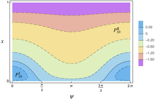
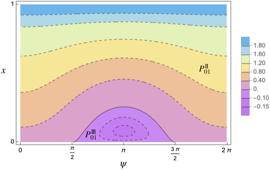
For a given pair , the bandgap is defined as the interval between the maximum of the acoustic frequency and the minimum of the optical frequency as the wave numbers run over the Brillouin triangle. In the linear case, since the gradients of and (with respect to ) never vanish in the interior of , maxima and minima are attained on the boundary . In particular, for every pair , the maximum of the linear acoustic frequency is attained at , while the minimum of the linear optical frequency is attained at . We anticipate that, in evaluating the nonlinear bandgap, the point plays a crucial role, more important than . Indeed, typically, in the set of parameters we are considering, namely the rectangle in the -plane, the displacement of the maximum of the acoustic frequency due to the nonlinearity is more relevant than that of the minimum of the optical frequency.
Resonant parameters
As in [DL], within the reference rectangle , we identify the curve formed by the pairs such that the linear acoustic and optical frequencies evaluated at are in 3:1 resonance, namely satisfy . is shown in Figure 26. In [DL], we identify the set of nonresonant pairs within the rectangle (represented by the light yellow region in Figure 26 (left)), for which the maximum/minimum of the nonlinear acoustic/optical frequencies on the boundary of the Brillouin triangle are attained at non resonant wave numbers , i.e. at points where the quantity is not small.
Formula (2.1) is valid in this nonresonant set, allowing us to directly evaluate the bandgap in [DL]. In contrast, in the complementary light purple zone in Figure 26, formula (2.1) is not applicable due to resonances and one has to use (153) as we will show here.
The final result of our analysis is presented in Figure 27, where the maximum percentage increment between the nonlinear and linear bandgap363636Namely , where and denote the width of the nonlinear and linear bandgap, respectively. is plotted as the pair varies over the rectangle in the softening case (). We emphasize that, while in [DL] we derived Figure 27 using (2.1) only for the pairs belonging to the light yellow set in Figure 26, in this section, we show how to derive it in the light purple set by (153).
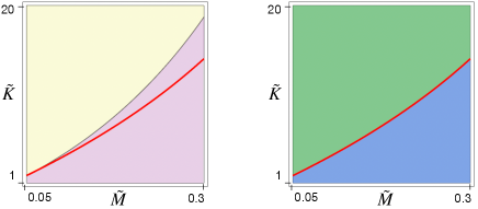
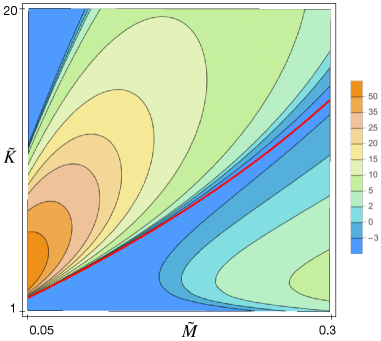
Let us first recall how in [DL] we identified the two regions in Figure 26 (left). Given a pair , we define a set in the -plane as resonant if every point in the set satisfies the 3:1 resonance condition . For a fixed pair within the rectangle (see Figure 26, (right)) there are always one or two resonant curves in the -plane, that intersect the Brillouin triangle (see Figure 28). The curve divides the rectangle into two regions: the one above and the one below , corresponding to the green region and the blue region in Figure 26 (right), respectively. For every fixed pair in the green region, there is only one resonant curve in the plane of wave numbers , that intersects the Brillouin triangle (the green curve in Figure 28). Conversely, for every fixed pair in the blue region, there are two resonant curves in the plane of wave numbers , that intersect the Brillouin triangle (the blue curves in Figure 28). Finally, in the limit case when the pair belongs to the curve , there are two resonant curves in the -plane, that intersect the Brillouin triangle, but one intersects only at (see the red curves in Figure 28).
Admissible amplitudes
Both in formula (2.1) and in formula (153), (recall also (155) and (156)), the nonlinear corrections to the frequencies are essentially proportional to the squares of the amplitudes and . Thus, the larger the amplitudes , the greater the displacement of the nonlinear bandgap relative to the linear one. On the other hand, (2.1) and (153) are perturbative in nature, as they are derived from the non resonant and resonant BNF, respectively. Therefore, must be sufficiently small for the formulae to remain valid. As shown in [DL], where they are analytically evaluated, the “admissible” amplitudes are smaller in the nonresonant case than in the resonant one. Indeed, since the nonresonant BNF cancels more terms, it is “stronger” than the resonant one. In particular the admissible amplitudes in the nonresonant case approach zero as the quantity vanishes. For example, when taking , the admissible amplitudes vanish for parameters values on the curve . This is not the case of the admissible amplitudes in the resonant case, namely the ones appearing in formulae (153), (155) and (156)). Indeed they are bounded away from zero on the resonances.
Shifting perspective, we can fix and observe at the variation of in the nonresonant case, as the wave numbers vary along the boundary of the Brillouin triangle . Notably, decreases to zero at certain resonant points, denoted . These points correspond to the intersections of the boundary of the Brillouin triangle with the resonant curves plotted in Figure 28. Formula (2.1) loses validity in the vicinity of any point . The values of the admissible initial amplitude (in the nonresonant case) as traverses are shown in Figure 29 for three different pairs of .
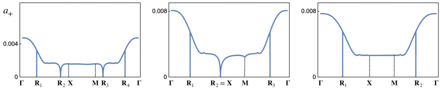
(On the left) Case (i): belonging to the light yellow region in Figure 26; admissible initial amplitudes , . As in the linear case, the maximum of the acoustic frequency is attained at , which is nonresonant. The resulting percentage bandgap increment is around .
(In the middle) Case (ii) belonging to the light purple region, more precisely to the red curve, in Figure 26; admissible initial amplitudes , . As in the linear case the maximum of the acoustic frequency is attained at , which, however, is now resonant. Since, at , is very close to , the resulting nonlinear bandgap undergoes a slight decrement compared to the linear case.
(On the right) Case (iii) belonging to the light purple region in Figure 26; admissible initial amplitudes are , . Since is almost flat around its maximum, the maximum of the nonlinear acoustic frequency is attained far from , more precisely near the resonant point . Since, close to , is very close to , the resulting nonlinear bandgap undergoes a decrement compared to the linear case.
In conclusion, due to the presence of the 3:1 resonance, formula (2.1) becomes invalid in the vicinity of the points , when the parameters are resonant or nearly resonant. Specifically, this occurs when they give rise to an exact, or nearly exact, 3:1 resonance between acoustic and optical frequencies. In this resonant case the correct expression for the nonlinear frequencies is , as given by (153).
Nonlinear bandgap
Let us consider the softening case; the hardening case
can be treated analogously,
leading to a general decrement of the bandgap.
We note that, since we are considering pairs
belonging to the rectangle ,
the point , where the minimum of the linear acoustic
frequency is attained, is always far from being resonant.
Therefore, in the following discussion, we will focus on
the maximum of acoustic frequency because
it undergoes the most significant displacements
and may be resonant.
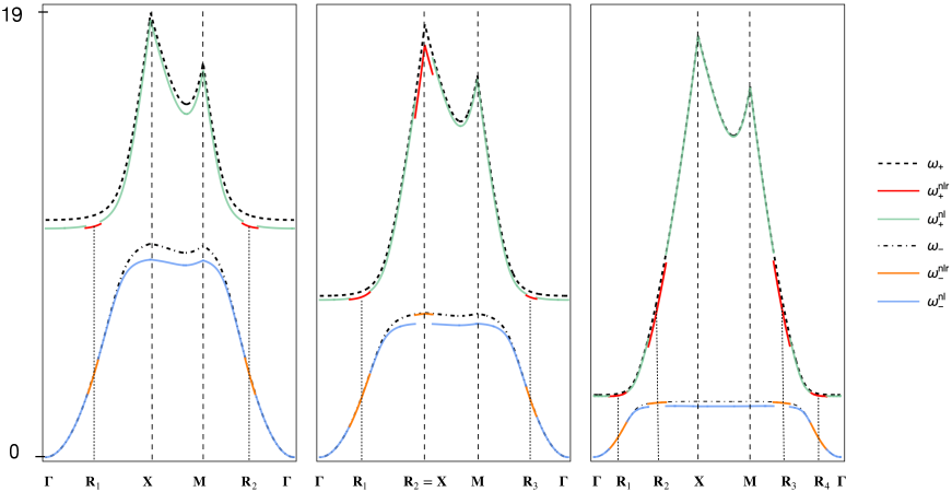
It turns out that, for the calculation of the nonlinear bandgap,
there are essentially three cases:
i) the maximum of the acoustic frequency
and the minimum of the optical frequency
are attained away from resonant
points,
ii) is resonant or nearly resonant,
iii) has an almost flat maximum,
so that, even if
is away from resonance,
the nonlinear acoustic frequency
may attain its maximum at
some resonant (or nearly resonant) point away from .
Note that
case i) corresponds to the
light yellow region in Figure 26,
while cases ii) and iii) correspond to the light purple
one.
These three cases are shown in Figure 30.
6 Conclusions
In this study, we investigated a broad range of structural engineering models by analyzing a general system of two coupled harmonic oscillators with cubic nonlinearity. Our examination revealed that, in the absence of damping, the system exhibits Hamiltonian dynamics, with an elliptic equilibrium at the origin characterized by two distinct linear frequencies.
In particular, we focused on the resonant or nearly resonant case,
specifically when the two frequencies are close to a 3:1 resonance.
Our investigation involved employing
Hamiltonian Perturbation Theory to transform the system into
(resonant) Birkhoff Normal Form up to order 4. This transformation provided a new set of symplectic action-angle variables,
on which the Hamiltonian, up to six-order terms, depends only
on the actions and the slow angle. Notably, our analysis highlighted the dependency of the construction on the system’s physical parameters, necessitating a meticulous case analysis of the phase portrait in the 3:1 resonant case. We found that
the system can exhibit up to six topologically different behaviors,
depending on the values of the physical parameters.
In each of these configurations,
we described the nonlinear normal modes
(elliptic/hyperbolic periodic orbits, invariant tori)
and their stable and unstable
manifolds of the truncated Hamiltonian (neglecting order six or higher terms). This is a fundamental step for proving the
persistence of the majority of these structures for the complete
Hamiltonian by KAM Theory.
By using elliptic integrals, we derived explicit analytic formulas for the nonlinear frequencies. While this analytic expression was already known away from resonances, it is, as far as we know, new in this context for the resonant or nearly resonant case.
As an application of our findings, we explored wave propagation in metamaterial honeycombs equipped with periodically distributed nonlinear resonators. Our investigation allowed us to examine the bandgap phenomenon in the presence of resonance. We found that while nonlinear effects far from resonances can significantly alter the bandgap, in the resonant case, the nonlinear frequencies, especially the acoustic one, closely align with the linear ones, resulting in a less pronounced variation in the bandgap.
7 Appendix
7.1 Proof of Proposition 1
We first count the solutions of equation (46),
namely the intersections between the line
and the function
in (47).
We note that, since is strictly convex,
if there is only one intersection.
Note that condition is equivalent
to .
Since , condition
implies that we are in the zones
or in which we have, indeed,
one intersection that we call
.
Moreover, in this case , the function
with has only one critical point, which is exactly .
This critical point is a minimum
since
and .
Assume now that .
Note that for every fixed
there exists a unique such that
is tangent to at some point
.
In order to evaluate the function
above let us consider
the tangent in a point to
; namely:
Since we want that we have to impose and . Since
| (157) |
imposing we have
| (158) | |||||
Note that:
| (159) |
Squaring we get
namely
The solutions of the above second order equation are
but by (159) we have to choose the minus sign. Since by (158) we have
by (157) and denoting for brevity , we get373737Note that .
| (160) | |||||
Note that .
Since we are in the case and
we have proved that the line
is tangent to ,
we have that for
there are not intersections (zone ) while for
there are two intersections (zone ),
that we call .
In this last case, the function
with has
two critical points, which are exactly
and
.
Since
and ,
must be a minimum
and
a maximum.
Finally the case
of equation (45)
and the critical points of the function
can be studied in the same way
sending and
.
∎
References
- [B20] Bukhari M., Barry O. Spectro-spatial analyses of a nonlinear metamaterial with multiple nonlinear local resonators, Nonlinear Dynamics, 99, pp. 1539–1560, 2020.
- [F22] Fortunati A., Bacigalupo A., Lepidi M., Arena A., Lacarbonara W. Nonlinear wave propagation in locally dissipative metamaterials via Hamiltonian perturbation approach, Nonlinear Dynamics 108, n.2, pp.765–787, 2022.
- [M23] Murer M., Guruva S. K., Formica G., Lacarbonara W. A multi-bandgap metamaterial with multi-frequency resonators, Journal of Composite Materials 57(4), 783-804 (2023).
- [SW23mssp] Shen Y., Lacarbonara Y. Nonlinear dispersion properties of metamaterial beams hosting nonlinear resonators and stop band optimization, Mechanical Systems and Signal Processing 187, 2023.
- [SW23jsv] Shen Y., Lacarbonara W. Nonlinearity-enhanced wave stop bands in honeycombs embedding spider web-like resonators, Journal of Sound and Vibration 562, 2023.
- [Guo22] Wenjie G., Zhou Yang, Qingsong Feng, Chengxin Dai, Jian Yang, Xiaoyan Lei A new method for band gap analysis of periodic structures using virtual spring model and energy functional variational principle, Mechanical Systems and Signal Processing 168, 2022.
- [Liu21] Liu Lei, Sridhar A., Geers M.G.D., Kouznetsova V.G. Computational homogenization of locally resonant acoustic metamaterial panels towards enriched continuum beam/shell structures, Computer Methods in Applied Mechanics and Engineering 387, 2021.
- [Cai22] Cai Changqi, Zhou Jiaxi, Wang Kai, Pan Hongbin, Tan Dongguo, Xu Daolin, Wen Guilin Flexural wave attenuation by metamaterial beam with compliant quasi-zero-stiffness resonators, Mechanical Systems and Signal Processing 174, 2022.
- [B16] Bacigalupo A., Gambarotta L. Simplified modelling of chiral lattice materials with local resonators, International Journal of Solids and Structures 83, 126–141, 2016.
- [Comi18] Comi C., Driemeier L. Wave propagation in cellular locally resonant metamaterials, Latin American Journal of Solids and Structures 15, 2018.
- [M22] Miranda Jr. E.J.P., Rodrigues S.F., Aranas Jr. C., Dos Santos, J.M.C. Plane wave expansion and extended plane wave expansion formulations for Mindlin-Reissner elastic metamaterial thick plates, Journal of Mathematical Analysis and Applications 2, 505, 2022.
- [Fan21] Fan Lei, He Ye, Chen Xiao-an, Zhao Xue A frequency response function-based optimization for metamaterial beams considering both location and mass distributions of local resonators, Journal of Applied Physics 11, 130, 2021.
- [Wang21] Wang Qiang, Li Jinqiang, Zhang Yao, Xue Yu, Li Fengming A frequency response function-based optimization for metamaterial beams considering both location and mass distributions of local resonators, Mechanical Systems and Signal Processing 151, 2021.
- [CP23] Chàvez-Pichardo M., Martìnez-Cruz M.A., Trejo-Martìnez A., Vega-Cruz A.B., Arenas-Resendiz T. On the Practicality of the Analytical Solutions for all Third- and Fourth-Degree Algebraic Equations with Real Coefficients Mathematics 11, 1147, 2023.
- [W] Lacarbonara W. Nonlinear Structural Mechanics: Theory, Dynamical Phenomena and Modeling, Springer, New-York, 2013.
- [Elliptic] Takebe T. Elliptic Integrals and Elliptic Functions, Moscow Lectures, Springer, 2022.
- [V07] Sanders J.A., Verhulst F., Murdock J. Averaging Methods in Nonlinear Dynamical Systems, Revised 2nd Edition, Springer, New York, 2007.
- [L19jsv] Fronk M. D., Leamy M. J. Direction-dependent invariant waveforms and stability in two-dimensional, weakly nonlinear lattices, Journal of Sound and Vibration 447, pp. 137–154, 2019.
- [M15] Malek S., Gibson L. Effective elastic properties of periodic hexagonal honeycombs, Mechanics of Materials 91, pp. 226–240, 2015.
- [S18] Sorohan S., Constantinescu D.M., Sandu M., Sandu A.G. On the homogenization of hexagonal honeycombs under axial and shear loading. Part I: Analytical formulation for free skin effect, Mechanics of Materials 119, pp. 74–91, 2018.
- [G97] Gibson L.J., Ashby M.F. Cellular solids: structure and properties, Cambridge Solid State Science Series, Cambridge University Press, 1997.
- [Graff] Graff S.M. On the conservation of hyperbolic invariant tori for Hamiltonian systems, J. Differential Equations 15, 1-69, 1974.
- [Val] Valdinoci, E. Families of whiskered tori for a-priori stable/unstable Hamiltonian systems and construction of unstable orbits, Math. Phys. Electron. J. 6, Paper 2, 31 pp., 2000.
- [MNT] Medvedev A.G., Neishtadt A.I., Treschev D.V. Lagrangian tori near resonances of near–integrable Hamiltonian systems, Nonlinearity 28 (7), pp. 2105–2130, 2015.
- [DL] Di Gregorio L., Lacarbonara W. On bandgaps sensitivity to 3:1 interactions between acoustic and optical waves, Preprint 2024.
- [H16] Haller G., Ponsioen S. Nonlinear normal modes and spectral submanifolds: existence, uniqueness and use in model reduction, Nonlinear Dynamics 86, pp. 1493–1534, 2016.
- [Cabre05] Cabre X., Fontich E., de la Llave R. The parametrization method for invariant manifolds III: overview and applications, J. Differential Equations 218, pp. 444–515, 2005.
- [Celletti13] Calleja R.C., Celletti A., de la Llave R. A KAM theory for conformally symplectic systems: Efficient algorithms and their validation, J. Differential Equations 255, pp. 978–1049, 2013.
- [Llave05] Haro A., de la Llave R. A parameterization method for the computation of invariant tori and their whiskers in quasi-periodic maps: Rigorous results, J. Differential Equations 228, pp. 230–279, 2005.
- [Fontich23] Fontich E., Vierio A. Dynamics near the invariant manifolds after a Hamiltonian-Hopf bifurcation, Communications in Nonlinear Science and Numerical Simulation 117, 2023, 106971.
- [Llave06] Haro A., de la Llave R. A parameterization method for the computation of invariant tori and their whiskers in quasi-periodic maps: numerical algorithms, Discrete and continuous dynamical systems Series B, 6 (6), pp. 1261–1300, 2006.
- [HW96] Haller G., Wiggins S. Geometry and chaos near resonant equilibria of 3-DOF Hamiltonian systems, Physica D 90, pp. 319–365, 1996.
- [HW95] Haller G., Wiggins S. N-pulse homoclinic orbits in perturbations of resonant Hamiltonian systems, Arch. Rat. Mech. Anal. 130, pp. 25–101, 1995.
- [HW93] Haller G., Wiggins S. Orbits homoclinic to resonances: the Hamiltonian case, Physica D 66, pp. 298–346, 1993.