Threshold phenomena for random discrete structures

To begin, we briefly introduce a model of random graphs. Recall that a graph is a mathematical structure that consists of vertices (nodes) and edges.

Roughly speaking, a random graph in this article means that, given a vertex set, the existence of each potential edge is decided at random. We will specifically focus on the Erdős-Rényi random graph (denoted by $G_{n,p}$), which is defined as follows.

Consider $n$ vertices that are labelled from 1 to $n$.

In reality, when we consider $G_{n,p}$, $n$ is a large (yet finite) number that tends to infinity, and $p=p(n)$ is usually a function of $n$ that tends to zero as $n\rightarrow\infty$. For example, $p=1/n$, $p=\log n/n$, etc.

We often use languages and tools from probability theory to describe/understand behaviors of $G_{n,p}$. Below we discuss some very basic examples.

We will write $f(n)\ll g(n)$ if $\frac{f(n)}{g(n)}\rightarrow 0$ as $n\rightarrow\infty$.

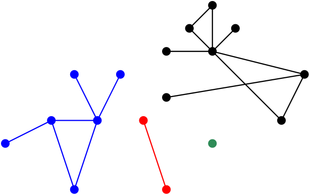
One striking thing about $G_{n,p}$ is that appearance and disappearance of certain properties are abrupt. Probably one of the most well-known examples that exhibit threshold phenomena of $G_{n,p}$ is appearance of the giant component. A component of a graph is a maximal connected subgraph. For example, the graph in Figure 4 consists of four components, and the size (the number of vertices) of each component is $1,2,6,$ and $8$.

For $G_{n,p}$, observe that, when $p=0$, the size of a largest component of $G_{n,p}$ is 1; in this case all of the edges are absent with probability 1, so each of the components is an isolated vertex. On the other hand, when $p=1$, $G_{n,p}$ is the complete graph with probability 1, so the size of its largest component is $n$.

Of course, one would naturally guess that as $p$ increases from $0$ to $1$, the typical size of a largest component in $G_{n,p}$ would also increase from 1 to $n$. But what is really interesting here is that there is a ”sudden jump” in this increment.

In the following statement and everywhere else, with high probability means that the probability that the event under consideration occurs tends to 1 as $n\rightarrow\infty$.

So around the value $p=\frac{1}{n}$, the giant component ”suddenly” appears, and therefore the structure of $G_{n,p}$ also drasitically changes. This is one example of the threshold phenomena that $G_{n,p}$ exhibits, and the value $p=\frac{1}{n}$ is a threshold function for $G_{n,p}$ of having the giant component. (The formal definition of a threshold function is given in Definition 2.3. See also the definition of the threshold in Section 5.)

The abrupt appearance of the giant component of $G_{n,p}$ is just one instance of vast threshold phenomena for random discrete structures. In this article, we will mostly deal with $G_{n,p}$ for the sake of concreteness, but there will be a brief discussion about a more general setting in Section 5.

Now we introduce the formal definition of a threshold function due to Erdős and Rényi. Recall that, in $G_{n,p}$, all the vertices are labelled $1,\ldots,n$. A graph property is a property that is invariant under graph isomorphisms (i.e. relabelling the vertices), such as $\{\text{connected}\}$, $\{\text{planar}\}$, $\{\text{triangle-free}\}$, etc. We use $\mathcal{F}(=\mathcal{F}_{n})$ for a graph property, and $G_{n,p}\in\mathcal{F}$ denotes that $G_{n,p}$ has property $\mathcal{F}$.

Note that it is not obvious at all whether a given graph property would admit a threshold function. Erdős and Rényi proved that many graph properties have a threshold function, and about 20 years later, Bollobás and Thomason proved that, in fact, there is a wide class of properties that admit a threshold function. In what follows, an increasing (graph) property is a property that is preserved under addition of edges. For example, connectivity is an increasing property, because if a graph is connected then it remains connected no matter what edges are additionally added.

On the other hand, knowing that a property $\mathcal{F}$ has a threshold function $p_{0}=p_{0}(\mathcal{F})$ does not tell us anything about the value of $p_{0}$. So it naturally became a central interest in the study of random graphs to find a threshold function for various increasing properties. One of the most studied classes of increasing properties is subgraph containment, i.e., the question of for what $p=p(n)$, $G_{n,p}$ is likely/unlikely to contain a copy of the given graph. Figure 8 shows some of the well-known threshold functions for various subgraph containments (and that for connectivity).

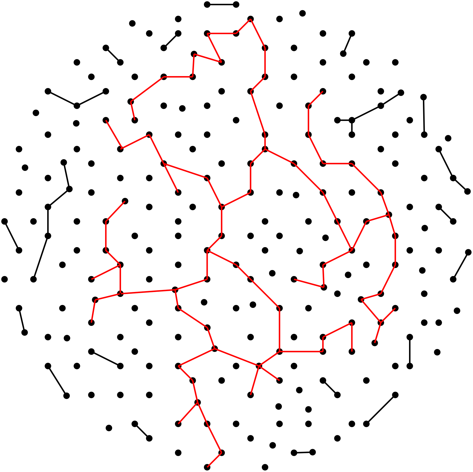
We stress that, in general, finding a threshold function for a given increasing property is a very hard task. To illustrate this point, let’s consider one of the most basic objects in graph theory, a spanning tree – a tree that contains all of the vertices.

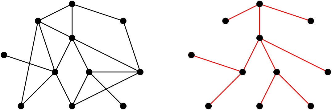
The question of finding a threshold function for $G_{n,p}$ of containing a spanning tree⁴⁴4This is equivalent to $G_{n,p}$ is connected. was one of the first questions studied by Erdős and Rényi. Already in their seminal paper [6], Erdős and Rényi showed that a threshold function for containing a spanning tree is $p_{0}=\frac{\log n}{n}$. However, the difficulty of this problem immensely changes if we require $G_{n,p}$ to contain a specific (up to isomorphisms) spanning tree (or more broadly, a spanning graph⁵⁵5A spanning graph means a graph that contains all of the vertices). For example, one of the biggest open questions in this area back in 1960s was finding a threshold function for a Hamiltonian cycle (a cycle that contains all of the vertices).

Note that both threshold functions for $\{$contain any spanning tree$\}$ and $\{\text{contain a Hamiltonian cycle}\}$ are of order $\frac{\log n}{n}$, even though the latter is a stronger requirement. Later we will see (in the discussion that follows Example 4.6) that $\frac{\log n}{n}$ is actually an easy lower bound on both threshold functions. It has long been conjectured that for any spanning tree⁶⁶6More precisely, for any sequence of spanning trees $\{T_{n}\}$ with a constant maximum degree, its threshold function is of order $\frac{\log n}{n}$. This conjecture was only very recently proved by Montgomery [14].

Henceforth, $\mathcal{F}$ always denotes an increasing property.

In 2006, Jeff Kahn and Gil Kalai [12] posed an extremely bold conjecture that captures the location of threshold functions for any increasing properties. Its formal statement will be given in Conjecture 4.11 (graph version) and Theorem 5.7 (abstract version), and in this section we will give an informal description of this conjecture first. All of the terms not defined here will be discussed in the forthcoming sections.

Given an $\mathcal{F}$, we are interested in locating its threshold function, $p_{0}(\mathcal{F})$.⁷⁷7We switch the notation from $p_{0}(n)$ to $p_{0}(\mathcal{F})$ to emphasize its dependence on $\mathcal{F}$. But again, this is in general a very hard task.

Kahn and Kalai introduced another quantity which they named the expectation threshold and denoted by $p_{\mathbb{E}}(\mathcal{F})$, which is associated with some sort of expectation calculations as its name indicates. By its definition (Definition 4.5),

and, in particular, $p_{\mathbb{E}}(\mathcal{F})$ is easy to compute for many interesting increasing properties $\mathcal{F}$. So $p_{\mathbb{E}}(\mathcal{F})$ provides an ”easy” lower bound on the hard parameter $p_{0}(\mathcal{F})$. A really fascinating part is that then Kahn and Kalai conjectured that $p_{0}(\mathcal{F})$ is, in fact, bounded above by $p_{\mathbb{E}}(\mathcal{F})$ multiplied by some tiny quantity!

The graph version of this conjecture (Conjecture 4.11) is still open, but the abstract version (Theorem 5.7) is recently proved in [15].

The conjecture of Kahn and Kalai is very strong, and even the authors of the conjecture wrote in their paper [12] that ”it would probably be more sensible to conjecture that it is not true.” The fundamental question that motivated this conjecture was:

Recall that the definition of a threshold (Definition 2.3) doesn’t distinguish constant factors. So in this section, we will use the convenient notation $\gtrsim,\lesssim$, and $\asymp$ to mean (respectively) $\geq,\leq$, and $=$ up to constant factors. Finally, write $p_{0}(H)$ for a threshold function for $G_{n,p}$ of containing a copy of $H$, for notational simplicity.

The next example shows that the above dream is too dreamy to be true.

In Example 4.3, $p_{0}(\tilde{H})$ is not predicted by the expected number of $\tilde{H}$, thus the Dream is broken. However, it still shows that $p_{0}(\tilde{H})$ is predicted by the expected number of some subgraph of $\tilde{H}$, and, intriguingly, this holds true in general. To provide its formal statement, define the density of a graph $F$ by

The next theorem tells us the exciting fact that we can find $p_{0}(F)$ by just looking at its densest subgraph, as long as $F$ is fixed.⁸⁸8For example, a Hamiltonian cycle is not a fixed graph, since it grows as $n$ grows.

For example, in Example 4.2, the densest subgraph of $H$ is $H$ itself, so $p_{0}(H)$ is determined by the expectation of $H$. This also determines $p_{0}(\tilde{H})$ in Example 4.3, since the densest subgraph of $\tilde{H}$ is again $H$.

Motivated by the preceding examples and Theorem 4.4, we give a formal definition of the expectation threshold.

Observe that

and in particular, Theorem 4.4 gives that

The existence of an isolated vertex in $G_{n,p}$ is essentially equivalent to the Coupon-collector’s Problem:

Observe that, in Example 4.6, the ”coupon-collector behavior” of $G_{n,p}$ provides another lower bound on $p_{0}(\text{PM})$, pushing up the first lower bound, $p_{\mathbb{E}}(\text{PM})$, by $\log n$. And it turned out that this second (better) lower bound is equal to the threshold.

To investigate this question, we consider a random process defined as below. Consider a sequence of graphs on $n$ vertices

where $G_{m+1}$ is obtained from $G_{m}$ by adding a random edge.

We remark that Theorem 4.8 gives much more precise information about $p_{0}(\text{PM})$ (back in $G_{n,p}$ setting). For example, Theorem 4.8 implies:

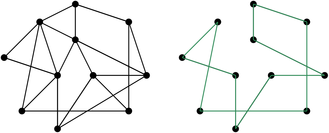
We observe a similar phenomenon for Hamiltonian cycles. Notice that in order for a graph to contain a Hamiltonian cycle, a minimum requirement is that every vertex is contained in at least two edges. The next theorem tells us that, again, this naive requirement is essentially the only barrier.

Returning to Question 4.1, so far we have established that there are two factors that affect threshold functions. We first observed that $p_{\mathbb{E}}$ always gives a lower bound on $p_{0}$. We then observed that, when it applies, the coupon-collector behavior of $G_{n,p}$ pushes up this expectational lower bound by $\log n$. Conjecture 4.11 below dauntingly proposes that there are no other factors that affect thresholds.

The question of a threshold function for a triangle-factor¹¹¹¹11or, more generally, a $K_{r}$-factor for any fixed $r$ was famously solved by Johansson, Kahn, and Vu [10]. Observe that an obvious obstruction for a graph from having a triangle factor is the existence of a vertex that is not contained in any triangles. The result below is the hitting time version of [10], which is obtained by combining [11] and [9].

The abstract version of the Kahn–Kalai Conjecture, which is the main content of this section, is recently proved in [15]. We remark that the discussion in this section is not restricted by the languages in graph theory anymore.

We introduce some more definitions for this general setting. Given a finite set $X$, the $p$-biased product probability measure, $\mu_{p}$, on $2^{X}$ is defined by

We use $X_{p}$ for the random variable whose law is

In other words, $X_{p}$ is a ”$p$-random subset” of $X$, which means $X_{p}$ contains each element of $X$ with probability $p$ independently.

We redefine increasing property in our new set-up. A property is a subset of $2^{X}$, and $\mathcal{F}\subseteq 2^{X}$ is an increasing property if

Informally, a property is increasing if we cannot ”destroy” this property by adding elements. Note that in this new definition, $\mathcal{F}$ is not required to possess the strong symmetry as in increasing graph properties; for example, there is no longer a requirement like ”invariant under graph isomorphisms.”

Observe that $\mu_{p}(\mathcal{F})(:=\sum_{A\in\mathcal{F}}\mu_{p}(A)=\mathbb{P}(X_{p}\in\mathcal{F}))$ is a polynomial in $p$, thus continuous. Furthermore, it is a well-known fact that $\mu_{p}(\mathcal{F})$ is strictly increasing in $p$ unless $\mathcal{F}=\emptyset,2^{X}$ (see Figure 20). For the rest of this section, we always assume $\mathcal{F}\neq\emptyset,2^{X}$.

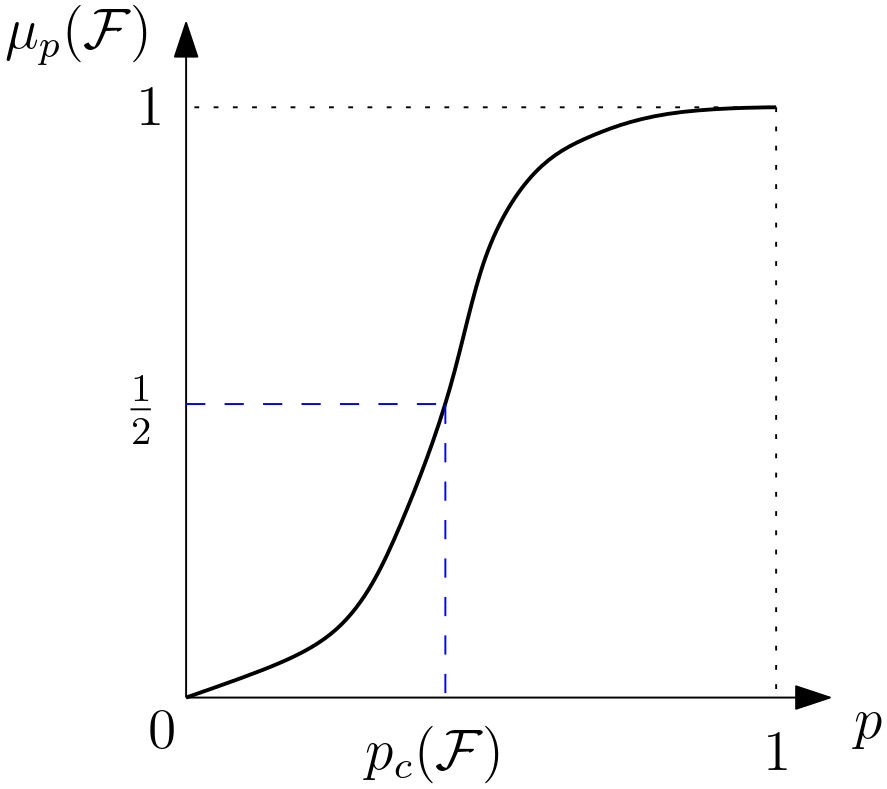
Because $\mu_{p}(\mathcal{F})$ is continuous and strictly increasing in $p$, there exists a unique $p_{c}(\mathcal{F})$ for which $\mu_{p_{c}}(\mathcal{F})=1/2$. This $p_{c}(\mathcal{F})$ is called the threshold for $\mathcal{F}$.

For a general increasing property $\mathcal{F}\subseteq 2^{X}$, the definition of $p_{\mathbb{E}}$ is not applicable anymore. Kahn and Kalai introduced the following generalized notion of the expectation threshold, which is also introduced by Talagrand [17].

The next proposition says that $q(\mathcal{F})$ still provides a lower bound on the threshold.

For a graph $F$, write $\mathcal{F}_{F}$ for the increasing graph property of containing a copy of $F$. The example below illustrates the relationship between $p_{\mathbb{E}}(F)$ and $q(\mathcal{F}_{F})$.

The above discussion shows that, for any (not necessarily fixed) graph $F$,

(whether $p_{\mathbb{E}}(F)\asymp q(\mathcal{F}_{F})$ is unknown). The abstract version of the Kahn–Kalai Conjecture is similar to its graph version, with $p_{\mathbb{E}}$ replaced by $q(\mathcal{F})$. This is what’s proved in [15].

Theorem 5.7 is extremely powerful; for instance, its immediate consequences include historically difficult results such as the resolutions of Shamir’s Problem [10] and the ”Tree Conjecture” [14]. Here we just mention one smaller consequence:

Note that $q(\mathcal{F})$ is in theory hard to compute. For instance, in Example 4.3, we can estimate $p_{\mathbb{E}}(\tilde{H})$ by finding $F\subseteq\tilde{H}$ with the maximum $e(F)/v(F)$. On the other hand, to compute $q(\mathcal{F}_{\tilde{H}})$, we should in principle consider all possible covers of $\mathcal{F}_{\tilde{H}}$, which is typically not feasible. The good news is that there is a convenient way to find an upper bound on $q(\mathcal{F})$, which is often of the correct order. Namely, Talagrand [17] introduced a notion of fractional expectation threshold, $q_{f}(\mathcal{F})$, satisfying

for any increasing property $\mathcal{F}.$ He conjectured (and it was proved in [8]) that the (abstract) Kahn-Kalai Conjecture (now Theorem 5.7) holds with $q_{f}(\mathcal{F})$ in place of $q(\mathcal{F})$. This puts us in linear programming territory: by LP duality, a bound $q_{f}(\mathcal{F})\leq\alpha$ ($\alpha\in[0,1]$) is essentially equivalent to existence of an ”$\alpha$-spread” probability measure on $\mathcal{F}$. In all applications of Theorem 5.7 to date, what is actually used to upper bound $q(\mathcal{F})$ is an appropriately spread measure.¹²¹²12The problem of constructing well-spread measure is getting growing attention now: see e.g. [13] for a start. So all these applications actually follow from the weaker Talagrand version.

We close this article with a very interesting conjecture of Talagrand [17] that would imply the equivalence of Theorem 5.7 and its fractional version:

References

- [1] M. Ajtai, J. Komlós and Szemerédi, The first occurrence of Hamilton cycles in random graphs, Annals of Discrete Mathematics, 27 (1985) 173-178. MR0821516
- [2] R. Alweiss, S. Lovett, K. Wu, and J. Zhang, Improved bounds for the sunflower lemma, Ann. of Math. (2) 194 (2021), no. 3, 795–815. MR4334977
- [3] B. Bollobás, The evolution of sparse graphs, Graph theory and combinatorics, Cambridge (1983), 35–57. MR0777163
- [4] B. Bollobás, Random Graphs, second ed., Cambridge Studies in Advanced Mathematics, vol. 73, Cambridge University Press, Cambridge (2001). MR1864966
- [5] B. Bollobás and A. Thomason, Threshold functions, Combinatorica 7 (1987), 35-38. MR0905149
- [6] P. Erdős and A. Rényi, On the evolution of random graphs, Publ Math Inst Hungar Acad Sci 5 (1960), 17-61. MR0125031
- [7] P. Erdős and A. Rényi, On the existence of a factor of degree one of a connected random graph, Acta. Math. Acad. Sci. Hungar. 17 (1966) 359-368. MR0200186
- [8] K. Frankston, J. Kahn, B. Narayanan, and J. Park, Thresholds versus fractional expectation-thresholds, Ann. of Math. (2) 194 (2021), no. 2, 475-495. MR4298747
- [9] A. Heckel, M. Kaufmann, N. Müller, and M. Pasch, The hitting time of clique factors, Preprint, arXiv 2302.08340
- [10] A. Johansson, J. Kahn, and V. Vu, Factors in random graphs, Random Structures Algorithms 33 (2008), 1–28. MR2428975
- [11] J. Kahn, Hitting times for Shamir’s problem, Transactions of the American Mathematical Society 375, no. 01 (2022), 627-668. MR4358678
- [12] J. Kahn and G. Kalai, Thresholds and expectation thresholds, Combin. Probab. Comput. 16 (2007), 495-502. MR2312440
- [13] D. Kang, T. Kelly, D. Kühn, A. Methuku, and D. Osthus Thresholds for Latin squares and Steiner triple systems: Bounds within a logarithmic factor, Transactions of the American Mathematical Society, to appear.
- [14] R. Montgomery, Spanning trees in random graphs, Adv. Math. 356 (2019), 106793, 92. MR3998769
- [15] J. Park and H. T. Pham, A proof of the Kahn–Kalai Conjecture, Journal of the American Mathematical Society, to appear.
- [16] L. Pósa, Hamiltonian circuits in random graphs, Discrete Math. 14 (1976), 359-364. MR0389666
- [17] M. Talagrand, Are many small sets explicitly small?, STOC’10 – Proceedings of the 2010 ACM International Symposium on Theory of Computing, 13-35, ACM, New York, 2010. MR2743011