Threshold Resummation for Polarized High- Hadron Production at COMPASS
Abstract
We study the cross section for the photoproduction process where the incident photon and nucleon are longitudinally polarized and a hadron is observed at high transverse momentum. Specifically, we address the “direct” part of the cross section, for which the photon interacts in a pointlike way. For this contribution we perform an all-order resummation of logarithmic threshold corrections generated by soft or collinear gluon emission to next-to-leading logarithmic accuracy. We present phenomenological results relevant for the COMPASS experiment and compare to recent COMPASS data.
I Introduction
To obtain information about the nucleon’s gluon helicity distribution and to explore its contribution to the proton’s spin is the main focus of several current experiments. One of the probes employed for this purpose at CERN’s COMPASS experiment is , where denotes a charged hadron produced at high transverse momentum. Kinematics for the process are chosen in such a way that the photons exchanged between the muon and the nucleon are almost real, so that the process effectively becomes . Its double-longitudinal spin asymmetry is directly sensitive to , thanks to the presence of the photon-gluon fusion subprocess . COMPASS has recently presented data for the spin-averaged cross section Adolph:2012nm for the process, as well as for its spin asymmetry Adolph:2015hta ; Levillain:2015twa .
Thanks to the produced hadron’s large transverse momentum, the process may be treated with perturbative methods. As is well known Klasen:2002xb , hard photoproduction cross sections receive contributions from two sources, the “direct” ones, for which the photon interacts in the usual pointlike way in the hard scattering, and the “resolved” ones, for which the photon reveals its own partonic structure. Both contributions are of the same order in perturbation theory, starting at , with the electromagnetic and strong coupling constants and . Next-to-leading order (NLO, ) QCD corrections for the spin asymmetry for have been derived in Refs. deFlorian1998 and Jaeger2003 ; Jaeger2005 for the direct and resolved cases, respectively.
As discussed in MelaniesPaper , in the kinematic regime accessible at COMPASS perturbative corrections beyond NLO are important. This is because typical transverse momenta of the produced hadron are such that the variable (with the muon-proton center-of-mass energy) is relatively large, . This means that the partonic hard-scattering cross sections relevant for are largely probed in the “threshold”-regime, where the initial photon and parton have just enough energy to produce a pair of recoiling high- partons, one of which subsequently fragments into the observed hadron. The phase space for radiation of additional gluons then becomes small, allowing radiation of only soft and/or collinear gluons. As a result, the cancelation of infrared singularities between real and virtual diagrams leaves behind large double- and single-logarithmic corrections to the partonic cross sections. These logarithms appear for the first time at NLO and then recur with increasing power at every order of perturbation theory. Threshold resummation Sterman1987 ; Catani:1989ne allows to sum the logarithms to all orders to a certain logarithmic accuracy. It was applied to the spin-averaged cross section at COMPASS at next-to-leading logarithm (NLL) level in Ref. MelaniesPaper , where the resummation of both the direct and the resolved contribution was performed. The resummed result for the cross section was found to be significantly higher than the NLO one, by roughly a factor two. Comparison to the COMPASS data reported in Adolph:2012nm showed that this enhancement is crucial for achieving good agreement between data and the perturbative-QCD prediction.
In the light of this result, it is clear that threshold resummation should also be taken into account in the theoretical analysis of the spin asymmetry measured at COMPASS Adolph:2015hta . is the ratio of the spin-dependent cross section and the spin-averaged one. Since the latter has already been addressed in MelaniesPaper , we will in this paper examine threshold resummation for polarized scattering. As a first step, we will consider the direct contributions to the cross section, which are simpler to analyze and also formally dominate over the resolved ones near partonic threshold. We plan to complete our resummation study for in a future publication by performing threshold resummation also for the resolved contribution in the spin-dependent case. We note that the resolved contribution to is structurally equivalent to hadronic scattering , for which threshold resummation was performed in the previous literature even for the polarized case deFlorian2007 . However, Ref. deFlorian2007 only addressed the simplified case when the cross section is integrated over all rapidities of the produced hadron, while in the present case we consider an arbitrary fixed rapidity. The techniques necessary for this were devloped in Almeida2009 ; MelaniesPaper and will be used here as well.
Our paper is organized as follows: In Section II we recall the general framework for the process in QCD perturbation theory. Section III collects all ingredients for the threshold resummed spin-dependent cross section. In Section IV we present phenomenological results for the spin-dependent and spin-averaged cross sections at COMPASS, as well as for the resulting longitudinal double-spin asymmetry. Finally, we conclude our paper in Sec. V.
II Photoproduction cross section in perturbation theory
We consider the process
| (1) |
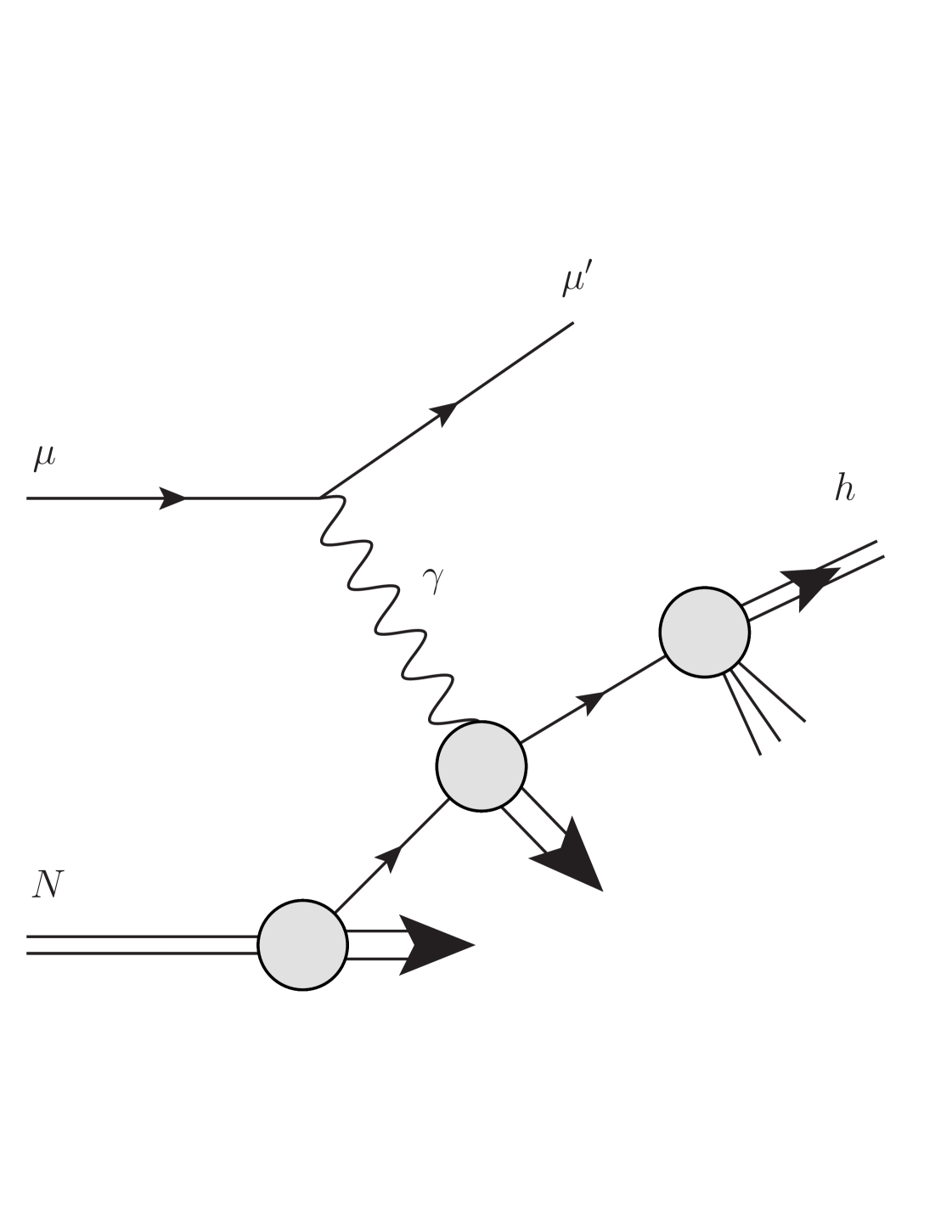
where the lepton and the nucleon are both longitudinally polarized and where a charged hadron is observed at high transverse momentum (see Fig. 1). Demanding the scattered lepton to have a low scattering angle with respect to the incoming one, the main contributions come from almost on-shell photons exchanged between the lepton and the nucleon. The scattering may then be treated as a photoproduction process , with the incoming lepton essentially serving as a source of quasi-real photons.
We introduce the spin-averaged and spin-dependent cross sections for the lepton-nucleon process as
| (2) |
where the superscripts , denote the helicities of the incoming particles. Using factorization, the differential spin-dependent cross section (as function of the hadron’s transverse momentum and pseudorapidity ) may be written as Jaeger2005 ; MelaniesPaper :
| (3) |
the sum running over all possible partonic channels . The are the polarized parton distribution functions of the nucleon, which depend on the momentum fraction carried by parton and on an initial-state factorization scale . They can be written as differences of distributions for positive or negative helicity in a parent nucleon of positive helicity,
| (4) |
In Eq. (3) we have introduced also “effective” parton distributions in a lepton, , which we shall elaborate on further below. For now we just note that in terms of spin-dependence they are defined exactly as in (4). The in (3) are the parton-to-hadron fragmentation functions that describe the hadronization of parton into hadron , with being the fraction of the parton ’s momentum taken by the hadron and a final-state factorization scale. Finally, the are the spin-dependent cross sections for the partonic hard-scattering processes . In analogy with (II) they are defined as
| (5) |
the indices now denoting the helicities of the incoming partons. The are perturbative and may hence be expanded in terms of the strong coupling constant ,
| (6) |
Apart from the partonic kinematic variables that will be introduced shortly, they depend on the factorization scales and also on a renormalization scale . We note that all formulas presented so far may be easily written for the spin averaged case by simply summing over helicities in (4),(5) instead of taking differences. This then gives the unpolarized cross section introduced in Eq. (II) in terms of the usual spin-averaged parton distributions and partonic cross sections .
In Eq. (3) we have introduced a number of kinematic variables. The partonic cross sections have been written differential in
| (7) |
with the Mandelstam variables
| (8) |
where are the four-momenta of the participating partons and where , with the lepton (nucleon) momentum (). Furthermore,
| (9) |
where , and the relationship between the hadron and the parton level center-of-mass system rapidities is
| (10) |
Finally, the lower integration bounds in Eq. (3) are given by
| (11) |
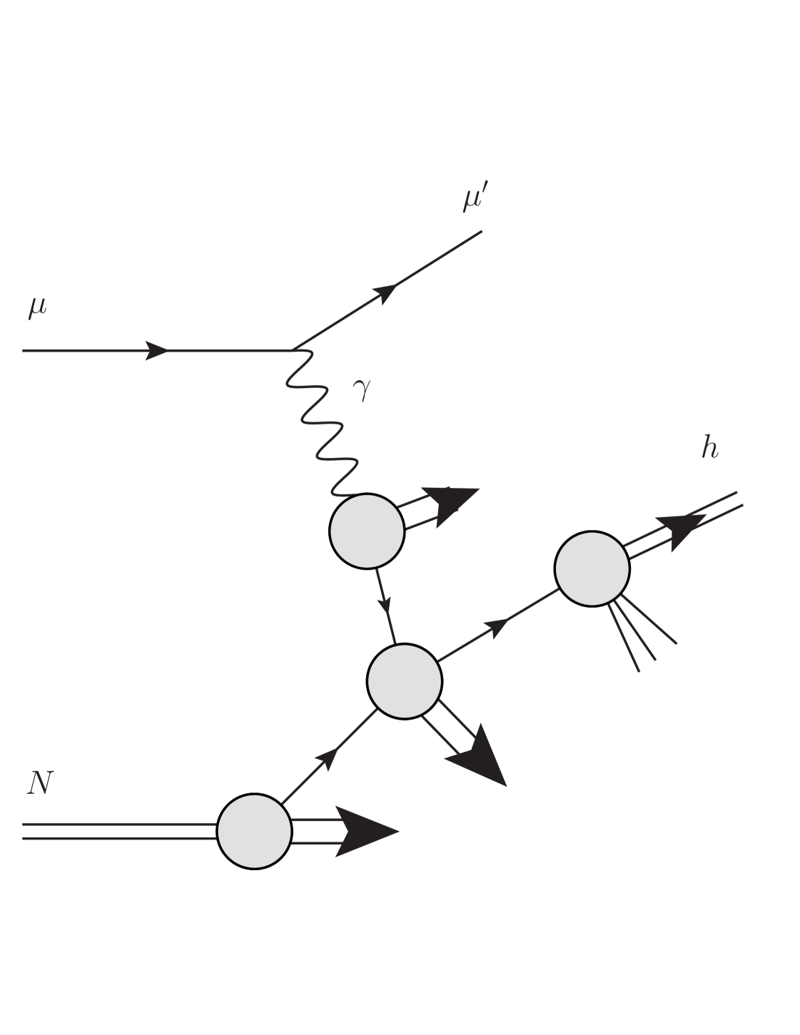
An important aspect of photoproduction cross sections is that the quasi-real photon can interact in two ways. For the direct contributions (see Fig. 1), it participates directly in the hard-scattering, coupling in the usual pointlike way to quarks and antiquarks. However, as is well established, the photon may also itself behave like a hadron, revealing its own partonic structure in terms of quarks, antiquarks, and gluons, as shown in Fig. 2. The associated contributions are known as resolved photon contributions. The physical cross section is the sum of the direct and the resolved part:
| (12) |
Both contributions are captured by Eq. (3) by introducing an effective spin-dependent parton distribution for the lepton:
| (13) |
where is the polarized Weizsäcker-Williams spectrum and describes the distribution of parton inside the photon. Equation (13) also applies to the direct case, see Fig. 1, where parton is an elementary photon and hence
| (14) |
The Weizsäcker-Williams spectrum is given by deFlorian:1999ge :
| (15) |
where is the fine structure constant. describes the (nearly) collinear emission of a polarized photon with momentum fraction by a polarized lepton with mass . The low virtuality of the photon is restricted by an upper limit that is determined by the experimental conditions.
In the direct case, there are three different LO subprocesses,
| (16) |
where the final-state particle in brackets is understood to remain unobserved, while the other parton fragments into the observed hadron. We note that the photon-gluon-fusion process is symmetric under exchange of and in the final state. The spin-dependent cross sections for the LO subprocesses are deFlorian1998 :
| (17) |
with , and the fractional electromagnetic charge of the quark.
In the resolved case, all QCD partonic processes contribute at LO:
| (18) |
where either of the final-state partons may fragment into the observed hadron. As the photon’s parton distributions are of order , both the direct and the resolved LO contributions are of order for the cross section (or of order for the one) Klasen:2002xb . Note that the contain a perturbative “pointlike” contribution that dominates at high , but also a nonperturbative “hadronic” piece that is associated with the photon converting into a vector meson and is important at low-to-mid .
As shown in Eq. (17), the LO partonic cross sections are proportional to . From (7) one finds that the invariant mass squared of the final state that recoils against the fragmenting parton is given by
| (19) |
The at LO thus reflects the fact that the recoil consists of a single massless parton. At NLO, the partonic cross sections contain various types of distributions in . Analytical expressions have been obtained in Refs. deFlorian1998 ; Jaeger2003 ; Jaeger2002 ; Aversa:1988vb ; Gordon:1994wu ; Hinderer:2015hra . For each process the result may be cast into the form
| (20) |
where the coefficients depend on the process under consideration, and where the plus-distributions are defined as usual by
| (21) |
The function in (20) contains all remaining terms without distributions in . The terms with plus-distributions give rise to the large double-logarithmic corrections that are addressed by threshold resummation. Their origin lies in soft-gluon radiation, and they recur with higher power at every higher order of perturbation theory. For the -th order QCD correction, the leading terms are proportional to (not counting the overall power of the partonic process in ). Subleading terms are down by one or more powers of .
Both the direct and the resolved contributions have the structure shown in (20). In the following we discuss the all-order resummation of the threshold logarithms in the direct part of the cross section, which we separate from the resolved part adopting the scheme. We perform the resummation to next-to-leading logarithm (NLL), which means that the three “towers” , , are taken into account to all orders in the strong coupling.
III Resummed cross section
III.1 Transformation to Mellin moment space
The resummation may be organized in Mellin moment space. A particularly convenient way developed in Almeida2009 ; MelaniesPaper is to start from Eq. (3) and write the convolution of the partonic cross sections with the fragmentation functions as the Mellin inverse of the corresponding products of Mellin moments. For the direct contributions we have
| (22) |
where
| (23) |
and
| (24) |
with as defined in (19). For simplicity, we have not written out the dependence of the on and on the factorization and renormalization scales, which they inherit from the . As one can see, in writing the cross section in the form (22) we keep the parton distribution functions in -space.
The plus-distributions in in the turn into logarithms of the Mellin variable in the . Specifically, the terms , , mentioned above turn into the NLL towers , , in moment space. Threshold resummation provides closed expressions for the that contain these logarithms to all orders. Inserting these expressions into (22) and performing the inverse Mellin transformation and the convolution with the parton distribution functions then yields the resummed hadronic cross section. We note that the presence of the moments of the fragmentation functions in (22) is important for making the Mellin-inverse sufficiently well-behaved that the convolution with the parton distribution functions can be carried out numerically. The reason is that the fall off rapidly at large and thus tame the logarithms in and hence the plus-distributions in .
III.2 NLL-resummed hard-scattering function
The resummed expressions for the may be obtained MelaniesPaper from the corresponding ones for the production of photons, , which were derived and discussed in detail in LaenenJuni1998 ; Sterman2000 ; Catani1998 . To NLL, one finds:
| (25) |
We now discuss the various functions appearing in this expression. We first note that among them only and depend on the polarizations of the incoming partons; all other factors are spin-independent. The are the Mellin-moments of the Born cross sections in (17):
| (26) |
We can easily compute them in closed form by exploiting the -function in (17) and the relation , Eq. (19). The coefficients match the resummed cross section to the NLO one. They correspond to hard contributions and primarily originate from the virtual corrections at NLO and may be extracted by comparing the exact NLO cross section with the first-order expansion of the resummed one. We have followed this procedure; our results are given in Appendix A. We note that the are functions of and the ratios , where is any of the scales .
The functions and in (25) account for soft radiation collinear to the initial-state parton or to the fragmenting parton , respectively. They are exponentials and given in the scheme as LaenenJuni1998
| (27) |
where the functions () are perturbative series in the strong coupling that are well-known. For convenience, we collect them in Appendix B. The function describes collinear emission, soft and hard, off the unobserved recoiling parton . We have LaenenJuni1998
| (28) |
Finally, emission of soft gluons at large angles is accounted for by the last factor in (25). The soft anomalous dimension in its exponent starts at LaenenJuni1998 ,
| (29) |
As indicated, it explicitly depends on the pseudo rapidity . The first-order terms of the anomalous dimensions for our various direct subprocesses can be obtained MelaniesPaper from those for the prompt-photon production processes, and , given in LaenenJuni1998 :
| (30) | ||||
| (31) | ||||
| (32) |
We note that the imaginary parts do not contribute since the real part is taken in the last exponent in (25).
After inserting all factors into Eq. (25), our final resummed expression is obtained by expanding to NLL. The techniques for this are standard, and we present the results of the expansion in Appendix B. We have checked that upon further expansion of the results to NLO, all single- and double-logarithmic terms of the exact NLO partonic cross sections given in deFlorian1998 are recovered. The terms constant in also match provided we use the coefficients as given in Appendix A.
We finally note that for the direct contributions that we consider in this paper, the LO hard-scattering cross sections only possess a single color structure, given by that of the vertex. Due to color conservation, soft-gluon emission thus cannot lead to color transitions in the hard-scattering subprocesses. This changes when one considers the resolved-photon contributions, for which at LO the QCD scattering processes in (II) contribute. As is well known deFlorian2007 ; KidonakisJan1998 ; Bonciani:2003nt ; deFlorian2005 ; Almeida2009 ; Hinderer:2014qta , in this case a matrix structure arises in the resummed cross section. We plan to address the resummation of the resolved-photon contributions in a future publication. We note that they are formally suppressed by relative to the direct ones near threshold, due to the photon’s parton distributions. As a result, they fall off more rapidly toward higher transverse momenta, as we shall see below.
III.3 Inverse Mellin transform and matching procedure
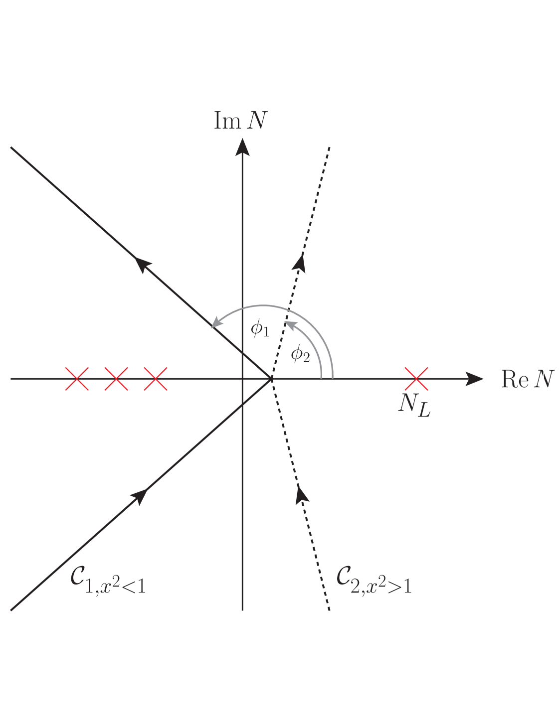
As seen in Eq. (25), we need to perform an inverse Mellin transform in order to arrive at the resummed hadronic cross section. In the course of this we need to deal with singularities appearing in the NLL expanded exponents, Eq. (B.5),(B.6), at and , where . These singularities are a consequence of the Landau pole in the perturbative strong coupling and lie on the positive real axis in moment space. The left of these poles is located at in the complex- plane. We will use the Minimal Prescription formula introduced in Catani_MinimalPrescr , for which one chooses the integration contour as shown in Fig. 3. The main feature of the contour is that it intersects the real axis at a value that lies to the left of (but, of course, to the right of all other poles originating from the fragmentation functions).
It is important to point out that the Mellin-integral in (25) defined in this way,
| (33) |
has support for both and . The latter contributions arise only because of the way the Landau poles are treated in the Minimal Prescription. They are unphysical in the sense that the cross section at any finite order of perturbation theory must not receive any contributions from . Mathematically, however, the unphysical contributions are needed to make sure that the expansions of the resummed cross section to higher orders in converge to the fully resummed result. We note that the piece with decreases exponentially with , so that its numerical effect is suppressed. As shown in Fig. 3, we tilt the contours with respect to the real axis, which helps to improve the numerical convergence of the Mellin integral. For (), we need to choose an angle ().
We finally note that as usual we match our resummed cross section to the NLO one by subtracting all NLO contributions that are present in the resummed result and adding instead the full NLO cross section:
| (34) |
where “” denotes the truncation at NLO. This procedure makes sure that NLO is fully included in the theoretical predictions, as well as all soft-gluon contributions beyond NLO to NLL accuracy. It avoids any double-counting of perturbative terms.
IV Phenomenological results
As discussed in the Introduction, measurements of cross sections and spin asymmetries for the photoproduction process are carried out in the COMPASS experiment Adolph:2012nm ; Adolph:2015hta at CERN. We therefore present our phenomenological results for COMPASS kinematics. COMPASS uses a longitudinally polarized muon beam with mean beam energy of GeV, resulting in GeV. Both deuteron and proton targets are available. COMPASS imposes the cut GeV2 on the virtuality of the exchanged photon which we use in the Weizsäcker-Williams spectrum (15). As in COMPASS, we also implement the cuts on the fraction of the lepton’s momentum carried by the photon, and for the fraction of the energy of the virtual photon carried by the hadron. Finally, charged hadrons are detected in COMPASS if their scattering angle is between mrad, corresponding to in the hadron’s pseudorapidity. We integrate over this range.
Our default choice for the helicity parton distributions is the set of deFlorian:2014yva (referred to as DSSV2014). We adopt the fragmentation functions of Ref. fDSS (DSS) throughout this work. In the calculations of the NLL resummed unpolarized cross sections we follow Ref. MelaniesPaper and use the numerical code of that work. Unless stated otherwise, we employ the unpolarized parton distribution functions of Ref. Martin:2009iq (referred to as MSTW). For comparisons we will also present results for the NLO resolved contributions, for which we will adopt the unpolarized and polarized photonic parton distributions of Refs. Gluck:1991jc and Gluck:1992zq , respectively. We furthermore choose all factorization/renormalization scales to be equal, . We usually choose , except when investigating the scale dependence of the theoretical predictions.
IV.1 Polarized and unpolarized resummed cross sections
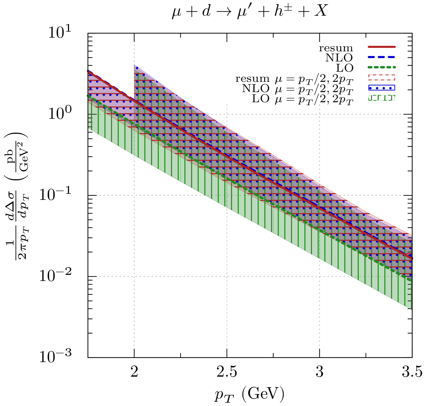
Figure 4 shows the direct parts (defined in the scheme) of the spin-averaged and spin-dependent cross sections for at leading order (LO), next-to-leading order, and resummed with matching implemented as described in Eq. (34). The symbols in the figure show the NLO-expansions of the non-matched resummed cross sections, and for comparison the figure also presents the NLO resolved contributions. We have summed over the charges of the produced hadrons. As can be seen, in the unpolarized case the difference between the LO and NLO results is very large, and resummation adds another equally sizable correction that increases relative to the NLO result as one goes to larger , that is, closer to threshold. The NLO expansion of the resummed cross section shows excellent agreement with the full NLO result, demonstrating that the threshold terms correctly reproduce the dominant part of the cross section. These findings are as reported in MelaniesPaper .
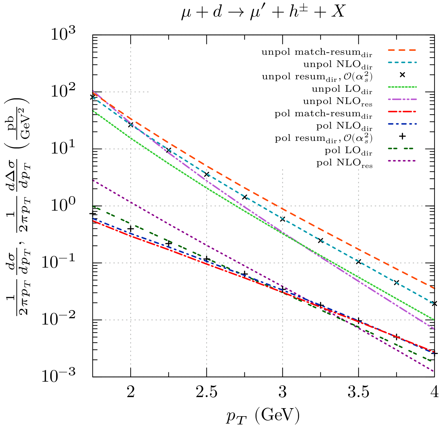
In the polarized case, the higher-order corrections are overall much more modest. The NLO prediction is slightly lower than the LO one at GeV but higher for larger values of transverse momentum. The resummation effects are smaller here, leading to only a modest further enhancement over NLO as one gets closer to threshold. This implies that the higher-order resummation effects will not cancel in the spin asymmetry for the process. Again the NLO expansion of the resummed cross section reproduces the full NLO result faithfully, although not quite as well as in the unpolarized case. These features that we observe for the direct part of the polarized cross section may be understood from the fact that the two competing LO subprocesses and enter with opposite sign and thus cancel to some extent. This was already observed in Ref. Jaeger2005 in the context of the NLO calculation. As discussed there, the cancelation is also responsible for the fact that the resolved contribution to the cross section computed with the “maximal” set of Gluck:1992zq is relatively much more important than in the unpolarized case, as is evident from the curves for the resolved part shown in the figure. Even though the resolved contributions also have gluon-initiated subprocesses and hence are sensitive to , they have significant uncertainty due to the fact that very little is known about the spin-dependent parton distributions of the photon. The (possible) dominance of the resolved contributions in the polarized case thus sets a severe limitation for extractions of from Jaeger2005 .
In Fig. 5 we examine the scale dependence of the spin-dependent cross section. For the resummed cross section we include the resolved contributions at NLO level, so that
| (35) |
The LO and NLO cross sections contain as usual their full direct and resolved contributions. We vary the scales in the range . One can observe that the scale uncertainty is large, especially so at the lower . There is a clear improvement when going from LO to NLO, but no further improvement when we include resummation. If anything, the resummed result shows a slightly larger scale dependence than the NLO one, a feature that will require further attention in the future.
IV.2 Double-Spin Asymmetry
We now investigate the double-longitudinal spin asymmetry for single-inclusive hadron production with a deuteron or a proton target. It is given by the ratio of the spin-dependent and the spin-averaged cross sections defined in Eq. (II):
| (36) |
We include the NLO resolved photon contributions, so that at the present stage the “resummed” spin asymmetry is given by
| (37) |
while the NLO one is as usual
| (38) |
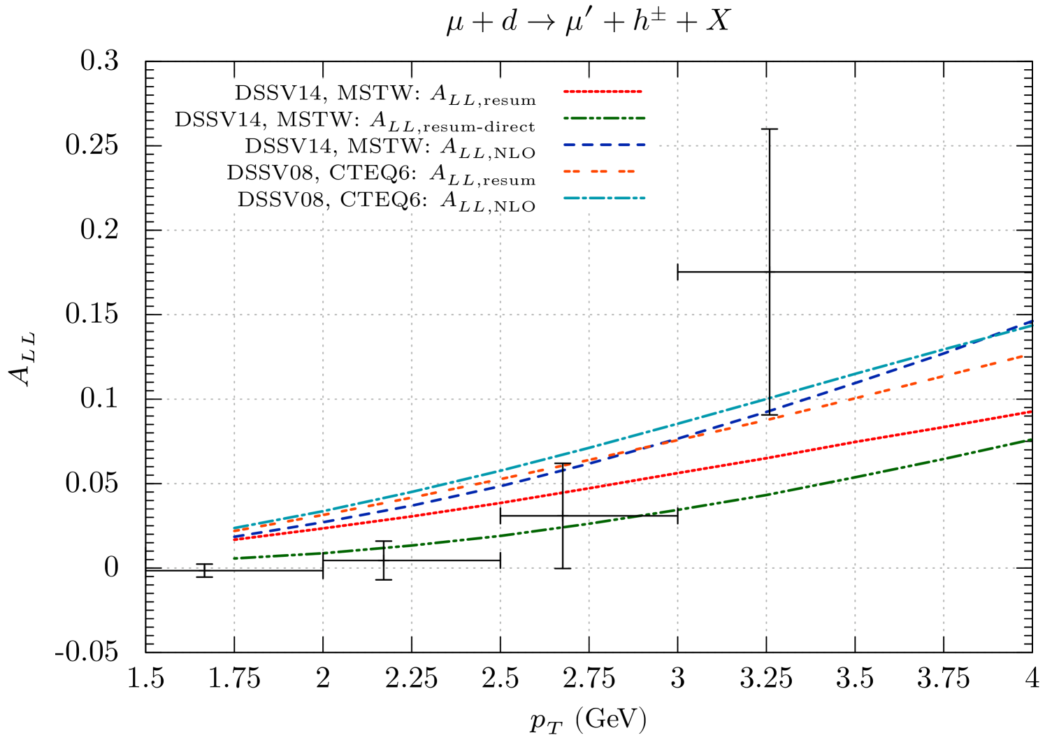
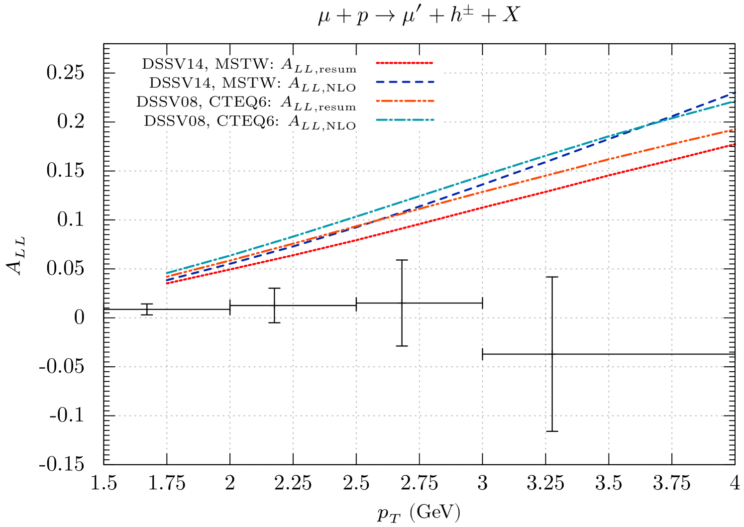
Our results are shown in Figs. 6 (a) and (b). The different size of the resummation effects for the polarized and unpolarized cross sections that we found in Fig. 4 clearly implies that the resummed threshold logarithm contributions do not cancel in the double-spin asymmetry. Indeed, as Fig. 6 shows, for our default sets of parton distributions the deuteron asymmetry is reduced by almost a factor of two at high , when going from NLO to the resummed case. For a proton target, there also is a substantial, albeit somewhat less dramatic, decrease. We also plot in the figure the corresponding results obtained by using the unpolarized and polarized parton distributions of Refs. CTEQ6M5 (CTEQ6.5M) and DSSV (DSSV2008), respectively. For these, the main trends are qualitatively similar, although the redcuction of is slightly less pronounced. This is likely due to the fact that the DSSV2008 set has a smaller gluon helicity distribution , so that the Compton process dominates, which has a positive partonic spin asymmetry and receives similar resummation effects in the unpolarized and the polarized case. We finally note that for the case of a deuteron target in Fig. 4 we also show the asymmetry based on the direct contributions alone. Evidently, this asymmetry is much smaller, expressing the fact that resolved contributions are likely very important for the polarized cross section.
As stated in the Introduction, COMPASS has recently presented data for the spin asymmetries for deuteron and proton targets Adolph:2015hta . The data (combined for the full rapidity range and summed over hadron charges) are shown in Fig. 6 in comparison to our theoretical results. As one can see, while the asymmetries for deuterons are in marginal agreement, the very small asymmetry seen by COMPASS for protons is incompatible with any of our predictions. It is worth mentioning that, as shown in Ref. Adolph:2015hta , this problem appears to be especially pronounced in the rapidity range and for positively charged hadrons. While the higher order resummed corrections that we have included ameliorate the situation, they are clearly not sufficient. Given the rather large decrease of the spin asymmetry generated by resummation of the direct contributions, it is arguably not possible to draw any reliable conclusions form this observation before also the resummation for the resolved part of the cross sections has been carried out. It appears unlikely, however, that the resolved contribution and its resummation will bring the data and theoretical results into good agreement since they affect the asymmetries for both targets in similar ways. If, for instance, the polarized resolved contribution were so large and negative that the proton data could be accommodated, the description of the deuteron asymmetry would vastly deteriorate Julius .
V Conclusions and outlook
We have studied the impact of threshold resummation at next-to-leading logarithmic level on the spin-dependent cross section for at high transverse momentum of the hadron , and on the resulting double-longitudinal spin asymmetry . For the present work, we have implemented the resummation only for the direct contribution to the cross section. For the kinematics relevant for the COMPASS experiment we find that the spin-dependent cross section receives much smaller enhancements by resummation than the spin-averaged one treated in Ref. MelaniesPaper . As a result, threshold effects do not cancel in the double-spin asymmetry, and the prediction for decreases when resummation is taken into account. Definite conclusions about the impact of resummation on the spin asymmetry will become possible only when also the resummation for the resolved component has been carried out, which we plan to do in future work. Only then will an extraction of the proton’s gluon helicity distribution become meaningful. We also note that the scale dependence of the perturbative cross section remains uncomfortably large even when resummation for the direct piece is taken into account. In order to improve this it may, eventually, be necessary to extend resummation to next-to-next-to-leading logarithmic level, following the techniques developed in Ref. Hinderer:2014qta .
Comparison to the recent COMPASS data Adolph:2015hta shows that the theoretically predicted spin asymmetries fail to reproduce the data well. Especially for the proton target the data show a nearly vanishing asymmetry, while the theoretical result appears to be always clearly positive. In fact, it is worth stressing that each of the theoretical results shown in Fig. 6 predicts a larger spin asymmetry for the proton than for the deuteron, in contrast to the trend seen in the data. This feature of the theoretical predictions is likely no accident, as a simple study of the LO direct contributions shows Julius . Clearly, future work is needed in order to clarify in how far the leading-twist perturbative-QCD framework can accommodate a larger spin asymmetry for than for .
Acknowledgements.
We are grateful to Y. Bedfer, F. Kunne, M. Levillain, C. Marchand, M. Pfeuffer, and J. Steiglechner for useful discussions. This work was supported by the “Bundesministerium für Bildung und Forschung” (BMBF) grants no. 05P12WRFTE and 05P12VTCTG.Appendix A Coefficients
In order to present our results for the in compact form, we define
| (A.1) |
where is the Euler constant. For the Compton process we then have
where . For the process with an observed gluon,
| (A.3) |
Finally, for photon-gluon fusion , we find
| (A.4) |
We note that is identical to the corresponding coefficient in the unpolarized case, which was given in MelaniesPaper .
Appendix B Radiative exponents and their expansion to NLL
The perturbative expansion of the function to the required order is given by
| (B.1) |
where for a quark and for a gluon, and where
| (B.2) |
with the number of flavors. The quark and gluon field anomalous dimensions and the leading terms of the diagonal splitting functions read to one-loop order LaenenJuni1998 :
| (B.3) |
where , with .
We next present the next-to-leading logarithmic expansions of and in Eqs. (27) and (28), respectively. Defining
| (B.4) |
we have Catani1998 ; Sterman2000 ; MelaniesPaper :
| (B.5) |
and
| (B.6) |
These exponents are universal in the sense that they depend only on the parton considered, but not on the overall subprocess. The functions and collect all leading logarithmic terms in the exponent, while the and produce next-to-leading logarithms . They read Catani1998
| (B.7) | ||||
| (B.8) |
with . Furthermore,
| (B.9) |
where .
References
- (1) C. Adolph et al. [COMPASS Collaboration], Phys. Rev. D 88, 091101 (2013) [arXiv:1207.2022 [hep-ex]].
- (2) C. Adolph et al. [COMPASS Collaboration], arXiv:1509.03526 [hep-ex].
- (3) See also: M. Levillain [COMPASS Collaboration], talk presented at the “12th Conference on the Intersections of Particle and Nuclear Physics (CIPANP 2015)”, Vail, Colorado, May 19-24, 2015; arXiv:1509.01419 [hep-ex].
- (4) See, for example: M. Klasen, Rev. Mod. Phys. 74, 1221 (2002) [hep-ph/0206169], and references therein.
- (5) D. de Florian and W. Vogelsang, Phys. Rev. D 57, 4376 (1998) [hep-ph/9712273].
- (6) B. Jäger, M. Stratmann and W. Vogelsang, Phys. Rev. D 68 (2003) 114018 [hep-ph/0309051].
- (7) B. Jäger, M. Stratmann and W. Vogelsang, Eur. Phys. J. C 44, 533 (2005) [hep-ph/0505157].
- (8) D. de Florian, M. Pfeuffer, A. Schäfer and W. Vogelsang, Phys. Rev. D 88, 014024 (2013) [arXiv:1305.6468 [hep-ph]].
- (9) G. F. Sterman, Nucl. Phys. B 281, 310 (1987).
- (10) S. Catani and L. Trentadue, Nucl. Phys. B 327, 323 (1989).
- (11) D. de Florian, W. Vogelsang and F. Wagner, Phys. Rev. D 76, 094021 (2007) [arXiv:0708.3060 [hep-ph]].
- (12) L. G. Almeida, G. F. Sterman and W. Vogelsang, Phys. Rev. D 80, 074016 (2009) [arXiv:0907.1234 [hep-ph]].
- (13) D. de Florian and S. Frixione, Phys. Lett. B 457, 236 (1999) [hep-ph/9904320].
- (14) B. Jäger, A. Schäfer, M. Stratmann and W. Vogelsang, Phys. Rev. D 67, 054005 (2003) [hep-ph/0211007].
- (15) F. Aversa, P. Chiappetta, M. Greco and J. P. Guillet, Nucl. Phys. B 327, 105 (1989).
- (16) L. E. Gordon, Phys. Rev. D 50, 6753 (1994).
- (17) See also: P. Hinderer, M. Schlegel and W. Vogelsang, Phys. Rev. D 92, 014001 (2015) [arXiv:1505.06415 [hep-ph]].
- (18) E. Laenen, G. Oderda and G. F. Sterman, Phys. Lett. B 438, 173 (1998) [hep-ph/9806467].
- (19) G. F. Sterman and W. Vogelsang, JHEP 0102, 016 (2001) [hep-ph/0011289].
- (20) See also: S. Catani, M. L. Mangano and P. Nason, JHEP 9807, 024 (1998) [hep-ph/9806484]; S. Catani, M. L. Mangano, P. Nason, C. Oleari and W. Vogelsang, JHEP 9903, 025 (1999) [hep-ph/9903436]; N. Kidonakis and J. F. Owens, Phys. Rev. D 61, 094004 (2000) [hep-ph/9912388]; D. de Florian and W. Vogelsang, Phys. Rev. D 72, 014014 (2005) [hep-ph/0506150]; T. Becher and M. D. Schwartz, JHEP 1002, 040 (2010) [arXiv:0911.0681 [hep-ph]].
- (21) N. Kidonakis and G. F. Sterman, Nucl. Phys. B 505, 321 (1997) [hep-ph/9705234]; N. Kidonakis, G. Oderda and G. F. Sterman, Nucl. Phys. B 525, 299 (1998) [hep-ph/9801268].
- (22) R. Bonciani, S. Catani, M. L. Mangano and P. Nason, Phys. Lett. B 575, 268 (2003) [hep-ph/0307035]; S. Catani, M. Grazzini and A. Torre, Nucl. Phys. B 874, 720 (2013) [arXiv:1305.3870 [hep-ph]].
- (23) D. de Florian and W. Vogelsang, Phys. Rev. D 71, 114004 (2005) [hep-ph/0501258].
- (24) P. Hinderer, F. Ringer, G. F. Sterman and W. Vogelsang, Phys. Rev. D 91, 014016 (2015) [arXiv:1411.3149 [hep-ph]].
- (25) S. Catani, M. L. Mangano, P. Nason and L. Trentadue, Nucl. Phys. B 478, 273 (1996) [hep-ph/9604351].
- (26) D. de Florian, R. Sassot, M. Stratmann and W. Vogelsang, Phys. Rev. Lett. 113, 012001 (2014) [arXiv:1404.4293 [hep-ph]].
- (27) D. de Florian, R. Sassot and M. Stratmann, Phys. Rev. D 75, 114010 (2007) [hep-ph/0703242 [hep-ph]].
- (28) A. D. Martin, W. J. Stirling, R. S. Thorne and G. Watt, Eur. Phys. J. C 63, 189 (2009) [arXiv:0901.0002 [hep-ph]].
- (29) M. Glück, E. Reya and A. Vogt, Phys. Rev. D 46, 1973 (1992).
- (30) M. Glück and W. Vogelsang, Z. Phys. C 57, 309 (1993); M. Glück, M. Stratmann and W. Vogelsang, Phys. Lett. B 337, 373 (1994).
- (31) W. K. Tung, H. L. Lai, A. Belyaev, J. Pumplin, D. Stump and C.-P. Yuan, JHEP 0702, 053 (2007) [hep-ph/0611254].
- (32) D. de Florian, R. Sassot, M. Stratmann and W. Vogelsang, Phys. Rev. Lett. 101, 072001 (2008) [arXiv:0804.0422 [hep-ph]]; Phys. Rev. D 80, 034030 (2009) [arXiv:0904.3821 [hep-ph]].
- (33) J. Steiglechner, Bachelor thesis, Tübingen Univ., 2015.