Tidal pull of the Earth strips the proto-Moon of its volatiles
Abstract
Prevailing models for the formation of the Moon invoke a giant impact between a planetary embryo and the proto-Earth (Canup, 2004; Ćuk et al., 2016). Despite similarities in the isotopic and chemical abundances of refractory elements compared to Earth’s mantle, the Moon is depleted in volatiles (Wolf and Anders, 1980). Current models favour devolatilisation via incomplete condensation of the proto-Moon in an Earth-Moon debris-disk (Charnoz and Michaut, 2015; Canup et al., 2015; Lock et al., 2018). However the physics of this protolunar disk is poorly understood and thermal escape of gas is inhibited by the Earth’s strong gravitational field (Nakajima and Stevenson, 2014). Here we investigate a simple process, wherein the Earth’s tidal pull promotes intense hydrodynamic escape from the liquid surface of a molten proto-Moon assembling at 3-6 Earth radii. Such tidally-driven atmospheric escape persisting for less than 1 Kyr at temperatures K reproduces the measured lunar depletion in K and Na, assuming the escape starts just above the liquid surface. These results are also in accord with timescales for the rapid solidification of a plagioclase lid at the surface of a lunar magma ocean (Elkins-Tanton et al., 2011). We find that hydrodynamic escape, both in an adiabatic or isothermal regime, with or without condensation, induces advective transport of gas away from the lunar surface, causing a decrease in the partial pressures of gas species () with respect to their equilibrium values (). The observed enrichment in heavy stable isotopes of Zn and K (Paniello et al., 2012; Wang and Jacobsen, 2016) constrain >0.99, favouring a scenario in which volatile loss occurred at low hydrodynamic wind velocities ( of the sound velocity) and thus low temperatures. We conclude that tidally-driven atmospheric escape is an unavoidable consequence of the Moon’s assembly under the gravitational influence of the Earth, and provides new pathways toward understanding lunar formation.
1 Introduction
While it is widely accepted that the Moon formed after a giant impact, the mechanisms by which it acquired its current physical state and composition remain debated (Canup, 2004; Ćuk et al., 2016; Nakajima and Stevenson, 2014; Lock et al., 2018; Cameron and Benz, 1991). Lunar mare basalts have refractory lithophile element ratios akin to terrestrial basalts but are invariably depleted in volatile and moderately volatile elements by a factor of (for alkali metals) to (highly volatile elements like Zn, Ag and Cd) relative to their terrestrial counterparts (Wolf and Anders, 1980; Ringwood et al., 1987; O’Neill, 1991; Lodders and Fegley, 2011; Day and Moynier, 2014). This depletion occurs in concert with enrichment in the heavy isotopes of moderately volatile elements including Zn (Paniello et al., 2012; Kato et al., 2015), K (Wang and Jacobsen, 2016; Tian et al., 2020), Cl (Sharp et al., 2007; Boyce et al., 2015; Gargano et al., 2020), Ga (Kato and Moynier, 2017), and Rb (Pringle and Moynier, 2017), indicative of an evaporative origin for volatile element loss from the Moon. Conversely, the enrichment of the lighter isotopes of Cr in lunar magmatic rocks compared to Earth’s mantle suggests devolatilisation occurred near equilibrium and under low temperatures ( 1800 K) (Sossi et al., 2018), far below those expected during a giant impact event.
Even under the extreme temperatures reached as a result of a giant impact (from to K Canup (2004); Ćuk et al. (2016); Nakajima and Stevenson (2014), the removal of volatile elements from the Earth-Moon system by thermal escape is inhibited because of (i) the Earth’s substantial gravitational field and (ii) the high molecular masses of the moderately volatile elements ( g/mol). Both cases are aggravated by the low abundance of hydrogen in the proto-Earth, preventing loss through aerodynamic drag (Nakajima and Stevenson, 2018). As such, recent models attempt to devolatilize Moon material prior to, or during, its assembly close to the Roche Limit within the post-impact debris disk (the ”protolunar disk”, a partially- to fully- vaporized disk). In the protolunar disk, volatile depletion by incomplete condensation and liquid-vapour partitioning may result from viscous separation of vapour from liquid (Charnoz and Michaut, 2015), or gravitational torque from the proto-Moon exerted on the vapour (Canup et al., 2015) or separation of growing melt droplets from the vapour due to gas-drag (Lock et al., 2018). However, these scenarios are critically dependent on the structure of the protolunar disk, which remains poorly understood, mostly due to its multi-phase nature and the unknown mixing states between gas and condensed phases (Thompson and Stevenson, 1988; Machida and Abe, 2004; Ward, 2012; Gammie et al., 2016; Charnoz and Michaut, 2015; Salmon and Canup, 2012; Lock et al., 2018). In some of these models, the protolunar disk is contained within the Earth’s Roche Limit, whereas numerical simulations of giant impacts show that most material ( by mass) is ejected beyond the Roche Limit (Nakajima and Stevenson, 2014) permitting volatile depletion beyond this point. The Roche Limit is the distance within which orbiting material cannot accrete into a single body due to disruption by the planets’ tides and is located at 3 Earth radii for silicate material orbiting the Earth.
Here, we present an alternative scenario for atmospheric loss from the proto-Moon assembling at Earth’s Roche limit. It is underpinned by the result that the influence of Earth’s tides lower the kinetic energy required for a gas to thermally escape from the proto-Moon (see next section), relative to that for the Moon considered in isolation in space. As a conceptual investigation of this process, model approximations were made in order to illustrate the first-order influence of tidally-assisted atmospheric escape on the chemical composition of the Moon. For all realistic model parameters, intense hydrodynamic escape is found to be inevitable from the proto-Moon, or its building blocks, provided it accreted at a distance of a few Earth’s radii such that Earth’s tides were sufficiently strong to lower the Moon’s escape velocity. We describe tidally-assisted thermal escape and show that, if the gas at the surface of the proto-Moon is hot enough to accelerate upwards to its Lagrange points, then this gas would be lost from the Moon, either by ejection into space, or by injection into orbit around the Earth. We explore two end-member scenarios, a ’wet’ and a ’dry’ model of the proto-lunar atmosphere, and show that, in both cases, the gas accelerates sufficiently through tidally-assisted thermal expansion to be able to escape. The gas velocity slows as the Moon’s orbital expansion causes the escaping flux to diminish. Over time, atmospheric loss via hydrodynamic escape produces a net depletion in the volatile element abundances in the Moon, consistent with measurements of lunar mare basalts.
The paper is organized as follows. In section 2 we examine, using simple arguments, under what conditions material may escape from the proto-Moon surface under the effect of tides. In section 3 we investigate two models of hydrodynamic escape assisted by tides and show that under all reasonable assumptions, escape is inevitable. In section 4 we discuss the orbital evolution of the proto-Moon, which sets an upper time limit for hydrodynamic escape to occur. In section 5 we compute the composition of the exsolved gas and the resulting melt composition. We show that it is possible to explain Na and K abundances in lunar records. We discuss our results and conclude in section 6.
2 A conceptual framework for atmospheric loss from the proto-Moon at the Roche Limit
Models of lunar assembly suggest that the Moon’s building blocks coalesce just beyond the Roche Limit (Canup et al., 2015; Takeda and Ida, 2001). Traditionally the Roche Limit for a fluid body , is (Roche, 1873; Canup and Esposito, 1995) :
| (1) |
where is the planet radius, is the planet density, and is the orbiting material density. For the case of the Earth, , and assuming the orbiting material has the same average density as the present-day Moon, we choose . These numbers give . Aggregates can begin to form at the edge of the proto-lunar disk around but the fully-grown Moon might appear further away, around (Canup et al., 2015; Salmon and Canup, 2012). The Moon’s gravitational attraction sphere is called the Hill Sphere and its radius is ( is the Earth-Moon distance, and are the masses of the Moon and Earth, respectively). We assume that the proto-Moon is hot and is surrounded by gas evaporated from its surface. If the proto-Moon’s atmosphere is contained within its Hill sphere, then it may be hydrostatically stable, like it is for the present-day atmospheres of the terrestrial planets. However, when the proto-Moon (or its building blocks) is located close to the Roche Limit, its Hill sphere has a size comparable to its physical radius ( km for a Moon located at ), meaning the atmosphere is hydrostatically unstable, and thereby liable to escape. Specifically, the Earth’s tidal pull lowers the minimum energy required for a particle to escape the proto-Moon’s surface (relative to the case for the Moon considered in isolation). The computation of the potential energy at the Moon’s surface, under Earth’s tidal field is detailed in Appendix A. As the L1 and L2 Lagrange points are the points on the Hill’s sphere closest to the Moon’s surface (Appendix A), escape of the gas is most readily achieved via passage through L1 and L2, because it requires the least energy 1). The kinetic energy required can be converted into a gas temperature 2. For this fiducial case, we assume a molar mass equal to g/mol, as a proxy for an atmosphere consisting of sodium Visscher and Fegley (2013)) . A well-mixed, static and transparent atmosphere in thermal equilibrium with the Moon’s hot surface at temperature (which is treated as a free parameter) is assumed, for simplicity, to produce a temperature profile that scales with , where is the distance to the Moon’s center and is the radius of the Moon (red lines in Figure 2). This scaling is simply obtained by equalizing the cooling power of a gas parcel, to the radiative power of a hot sphere at at distance : where L is the luminosity of the hot sphere (this is, for example, a common scaling in passive protoplanetary disk studies).
Under these simplistic assumptions, we find that, if the atmosphere is hot enough to escape beyond the Hill sphere when the proto-Moon is located at distance . Moreover a smaller proto-Moon (0.5 lunar mass), or its constituents, are more liable to atmospheric loss under the same conditions at same surface temperature (Figure2. b).
Whether the escaping atmosphere is permanently lost hinges upon the dynamics of the material after leaving the Moon’s Hill sphere. Classical celestial mechanics (Murray and Dermott, 1999) constrain outgoing particles to pass through either the L1 or L2 Lagrange points before being ejected into orbits around the Earth. The fate of this escaping material depends on the nature of the physical processes acting upon it. If the escaping material is gaseous, it does not re-accrete onto the Moon. That is, any dissipative process like gas viscosity or radiative cooling prevents the gas from re-entering the Hill Sphere because of a loss of mechanical energy. This is illustrated in Figure 3 (left) and Figure 4 where trajectories of particles leaving the Moon in a fictive gaseous disk were tracked and computed. It is observed that they do not fall-back onto the Moon, but rather migrate inward or outward, leaving the Moon permanently.
Alternatively, if the Earth’s surface is sufficiently hot during assembly of the proto-Moon ( K) (Canup, 2004; Ćuk et al., 2016; Nakajima and Stevenson, 2014) with a photosphere around 2000 K, then black-body emission may induce radiation pressure on micrometer-sized particles (in addition to heating the near-side of the proto-Moon). This leads to their ejection from the Earth-Moon system (Hyodo et al., 2018) (Figure 3, right and Figure 5). This scenario of ejection strongly depends on the physical size of dusty-grains. Here it is noted that escape is efficient for particles in the micrometer range from a Moon surface heated to 1500K following a giant impact (Appendix B).
We conclude from the first-order considerations detailed above that it is reasonable to expect that tidal effects would (1) facilitate the escape of material from the Moon’s surface and (2) prevent its return to the lunar surface due to 3 body-effects. Although the above-mentioned scenarios (dissipative gas disk, radiation pressure) may prevent the return of escaping material onto the Moon’s surface, the ”bottleneck” is to understand how material can be transported from the proto-Moon’s surface (i.e., the locus of its evaporation) up to the L1/L2 Lagrange points at which this material can escape.
3 Tidally-assisted hydrodynamic escape
Mechanisms capable of carrying gas from the molten proto-lunar surface to the escape points are a product of the thermochemical structure of its atmosphere. We investigate the mode of atmospheric escape occurring under the influence of the tidal pull of the Earth, and derive expressions that permit calculation of the escaping flux. To do so, we formulate two end-member scenarios using a 1D approach and take into account (1) evaporation from a magma ocean at surface temperature , and (2) the mutual gravitational attraction between the Earth and the Moon. Contrary to the abundant literature on planetary atmospheric escape, the atmosphere we consider here is not heated from above by an incoming XUV flux (see SI L), but rather from its base by a hot magma ocean, considered to be at constant temperature . In the first ”dry” model we assume a purely adiabatic gas evaporated from the magma ocean and neglect condensation during its adiabatic expansion (Section 3.1). The second ”wet” model assumes that individual species comprising the atmosphere may condense as liquid droplets depending on its pressure-temperature structure, and can be subsequently dragged along with the prevailing outflow (Section 3.2). Each of these scenarios involves simplifying assumptions to render calculations tractable, and the reality of atmospheric escape probably lies in between these two extremes. However, we use these two end-member scenarios as a proof-of-concept that tidally-driven thermal degassing is unavoidable under all reasonable assumptions, provided the proto-Moon assembles close to the Roche Limit.
In the following, it is assumed that the proto-Moon (or its building blocks) is surrounded by an atmosphere. The surface of the proto-Moon is assumed to be always liquid, and, in contact with the gas. We examine under which conditions the atmosphere can escape from its Hill sphere by solving the hydrodynamic equations, and considering the Earth’s tidal force.
3.1 Dry expanding atmosphere
Due to the intrinsic complexity of the physical process we aim to investigate, it is not feasible to treat the full problem self-consistently. We are mindful that, due to the temperature diminution with altitude, some fraction of the gas may recondense, and thus may not behave adiabatically. This case is treated in Section 3.2. However, it is of primary importance to first understand the physics of hydrodynamic escape above the lunar magma ocean by solving the fully adiabatic approximation, as it is the original (and natural) framework of the theory of hydrodynamic escape (Parker, 1963, 1965), and hence the crux of the present paper. Since the atmosphere is thin (at most 100 Pa) and composed largely of monatomic gases, it is reasonable to start with the adiabatic approximation, since acceleration is strong at the base of the atmosphere. However, for the sake of completeness, isothermal solutions are also presented in Appendix E.
3.1.1 Mathematical treatment
The derivation of the mass flux in the dry model is solved within the adiabatic approximation, thus we ignore here any condensation process during the escape of the gas from the proto-Moon’s surface, as well as heat transfer with the surroundings. We solve the Euler equations (conservation of mass and momentum + adiabatic equation of state) and calculate the 1D flow along the line joining the lunar surface to the Lagrange L1 or L2 points (located at the Hill radius). The gas follows the adiabatic equation of state, so that
| (2) |
where P is the total gas pressure, is a positive constant, is the adiabatic index ( , corresponding to a gas with a mixture of monatomic - = 5/3- and diatomic species = 7/5), where P is given by the sum of partial pressures of a gas produced in equilibrium with a magma of Bulk Silicate Earth (BSE) - like composition (Palme and O’Neill, 2003). These properties are related to the temperature via the adiabatic relation:
| (3) |
where and k are the mean molecular weight and Boltzmann’s constant, respectively. The molar mass of the gas is assumed to be (so . This corresponds roughly to a mixture of Na, O2 and K that are the dominant species for . At steady state, the conservation of mass reads :
| (4) |
Conservation of momentum for a steady-state flow reads:
| (5) |
where A(r) is the local acceleration in the non-inertial frame rotating with the Moon (Equation A2 in Appendix A). Equations 2 to 5 form a closed set of ODEs. The famous Bernoulli equation for an adiabatic gas is recovered by integrating equation 5 from the surface (subscript S) to the Hill sphere (subscript H) to obtain:
| (6) |
where is the potential energy in the frame rotating with the Moon. In the above Bernoulli equation, V and are linked through the mass conservation equation so that . Replacing in the Bernoulli equation one finally obtains:
| (7) |
where . Note that Equation 7 can also be written as follows :
| (8) |
with and standing for the gas temperature at the surface and at the Hill sphere, by inserting Equation 3 into Equation 7. It shows that the velocity field is independent of the surface pressure and is controlled only by the surface temperature and the gravity field. So for a given surface velocity and temperature , the velocity at the crossing of the Hill sphere can be determined by numerically solving equation 8. This is a well known problem for the case of a point-source gravity field and has been extensively treated by E.N. Parker in a series of papers on solar wind outflows (see e.g. Parker 1963).
The Bernoulli equation gives rise to several families of solutions extensively discussed in Parker (1963) and Parker (1965). The only physical solutions are those which start from the surface with flow velocities smaller than the sound speed. Then the velocity increases with height, passing through the transonic point beyond which the flow velocity becomes supersonic (but without a shock). All other solutions correspond either to inflow solutions (subsonic at large distance, supersonic on the ground) or do not connect the surface with infinity, or have finite pressure at infinity (see Parker 1965 for a detailed discussion).
The location of the transonic point is found as follows: inserting equation 4 into equation 5 and replacing by , and using Equation 3 one obtains:
| (9) |
For v(r) to be physical, the denominator and numerator must cancel simultaneously (this is the transonic point). Finding the zero of the denominator gives v at the sonic point (), and finding the zero of the numerator, and noting that along a current line, gives the location () and temperature of the sonic point. Once and are determined, the velocity at the Moon’s surface is determined by solving equation 7 between the sonic point and the surface, and the velocity at the Hill sphere is obtained by solving the Bernoulli equation between the sonic point and the Hill sphere. One unknown still needs to be determined: the gas density at the sonic point. In order to do so, we prescribe the surface temperature. Since the velocity field is independent of density (Equation 8) V can be computed everywhere starting from the sonic point. Once the velocity field is found, the density and pressure at the surface of the magma ocean must be determined (see next section), in order to obtain the net escaping flux.
3.1.2 Determining the gas density at the evaporating surface
We now focus on the determination of the surface flux, which depends on the evaporative flux at the ocean magma surface (+) and on the return flux back to the magma ocean (-), with the difference being the net flux away from the surface. The evaporative flux can be determined by the Hertz-Knudsen-Langmuir (HKL) equation (e.g. Knudsen, 1909) integrated over the surface area of the Moon, and is proportional to the equilibrium partial pressure of the gas () that can be calculated thermodynamically. The subsequent transport of this gas away from the surface occurs by molecular motion through two distinct mechanisms; advection and diffusion, or a combination thereof. If this transport rate is slow relative to the evaporation rate, there is a ’return flux’ to the surface, which, in turn, results in a build up of the partial pressure (or density) at this surface () owing to mass conservation (Richter et al. (2002); Young et al. (2019); Tang and Young (2020)). This is a classical feature of the HKL equation (the term), though it does not explicitly prescribe how is calculated. An expression for calculating the return flux (and thus the term) is proposed in Young et al. (2019); Tang and Young (2020), following the Richter et al. (2002) approach. Because Young et al. (2019); Tang and Young (2020) assume there is a surface boundary layer directly above the magma ocean that is well-mixed and in hydrostatic equilibrium, diffusion is the only possible mode of mass transport within this layer. In this approach, diffusive transport is derived from Fick’s Law, in which the diffusion coefficient for a binary gas is given by the Chapman-Enskog equation. This model always results in values that are very close to unity (i.e., equilibrium between the magma and the gas) because diffusion is exceedingly slow when integrated over the Moon’s surface area. While self-consistent, such an approach is not applicable for cases in which advection occurs at the surface, as described here. A suitable expression for an advected gas is derived in Appendix D, where we compute the return flux, as well as pressure and density of a gas at the surface of an evaporating surface, taking into account advection. We use a kinetic approach very similar to the original Hertz-Knudsen theory. We show that surface pressure and density depend only on the ratio of the gas velocity at the surface to the local thermal velocity . It is found that the gas density above the fluid surface () is (Equation D14 in appendix D) :
| (10) |
where is the gas density at saturation and at temperature is the saturating vapour pressure of a magma of BSE composition at temperature given in Visscher and Fegley (2013). We start by computing the velocity profile using the Bernoulli equation. This permits the surface velocity to be calculated, and the density and pressure at the surface are then computed using Equation 10. The escaping flux is given as . Here we assume for simplicity that the solid angle of gas emission is 1 steradian (compared to for a full sphere). Finally, one obtains a velocity profile with a mass flux that is perfectly conserved, allowing a precise estimate for the return flux to the surface to be made.
3.1.3 Results
Figure 6 shows the ratio of surface velocity to thermal velocity, for different surface temperatures, as a function of the Earth-Moon distance. We see that for all cases considered and thus the surface pressure is always (see appendix D), but for (our preferred case), never exceeds , meaning the surface pressure is always . Therefore, the actual surface pressure is found to lie close to gas-liquid equilibrium. In our case, and contrary to comets, the atmosphere expands at velocities much lower than the thermal velocity. Values reported in Figure 6 also imply that the net escaping gas flux from the proto-Moon is small compared to the free evaporative flux from the magma ocean (the ratio of the two being displayed in Figure 23), apart from cases in which and where the escaping flux becomes about half of the free evaporative flux.
The resulting escape fluxes are displayed in 7. The flux of escaping gas drops with increasing Earth-Moon distance up to the point where escape becomes negligible because of the diminishing gravitational influence of the Earth that otherwise promotes escape. For a lunar surface temperature of 2200 K, the atmosphere of the proto-Moon is efficiently lost provided the proto-Moon is located inward of 5, with a flux varying between Moon masses/year at to the Roche limit, down to Moon mass/year at 5.5. For K the flux is much lower, between and Moon mass/year at 3.7 only, due to the lower internal energy of the escaping gas. Note that the fluxes reported above may be underestimated, as we assume (for simplicity) the gas emitting surface is only 1 steradian, one order of magnitude smaller than a fully degassing spherical surface ( steradians). This conservative lower bound is justified due to the uncertainty of the areal extent of a lunar magma ocean, together with the fact that the mathematical treatment outlined above strictly applies only along the Earth-Moon line (L1 and L2 Lagrange points).
If we consider potential lunar buildings blocks with half a lunar mass, the flux is more intense by about a factor 2 to 5 (Figure 8), and, interestingly escape is arrested, on average, at a distance about twice as far from the Earth compared to a fiducial lunar mass. Thus, hydrodynamic escape from a 0.5 lunar mass proto-Moon at 1600 K occurs up to about 6.4 (compared to 3.7 for a 1 lunar mass object), and beyond 10 for a surface temperature of 2000K.
3.2 Wet model with condensation
The dry model presented above neglects any condensation or drag of silicate and oxide droplets. Condensation may affect the escape flux due to internal energy transfer within the atmosphere associated with the latent heat of condensation. To account for this, we have developed a wet model that includes gas condensation. We calculate the composition of the vapour phase presuming it is in equilibrium with a liquid of Bulk Silicate Earth (BSE) composition whose renewal timescale at the surface of the magma ocean is very short ( days, see Appendix F) relative to the cooling timescale.
3.2.1 Mathematical treatment
We introduce a method to compute the velocity field and composition of the escaping atmosphere. The treatment is not fully self-consistent as we treat each species as pure (i.e. they have the same speciation in both the condensed and the gas phase), however this approach still represents a significant advance compared to the state-of-the-art, as we consider a multicomponent atmosphere in dynamical flow following a moist-adiabat. Whereas the computation of a steady-state atmospheric structure taking into account a moist adiabat is common, the present work is, to our knowledge the first work that explicitly computes the composition of the atmosphere during its escaping trajectory and for a mixture of species.
3.2.2 Calculation of the (P,T) structure
During gas expansion leading to escape, we assume that the mixture (comprised of gas and condensates) outgassed from the Moon’s surface follows a moist adiabat, that is, the mixture cools adiabatically with condensates remaining bound to the gas (as justified in Appendix C), leading to a specific (P,T) or (,T) relation that depends only on the initial entropy and composition of the mixture at the Moon’s surface. Here we calculate the (P,T) and (,T) relations for a given mixture composition and temperature at the Moon’s surface. We consider a mixture including N species that can be either in gaseous or condensed form. We consider two stages during hydrodynamic escape of the gas. First, the temperature drops isentropically from that of the magma ocean, , to some temperature, , with no heat exchange with the surroundings. When the gas has cooled sufficiently to reach a lower threshold temperature , we assume that the mixture of gas and dust is heated by the Sun in order to maintain a constant temperature. is therefore simply assumed to be the equilibrium temperature at the location of the Earth-Moon system in the absence of greenhouse heating: 250 K. This is an approximation; in order to compute the true temperature self-consistently, we would need to couple our hydrodynamic/chemical system to a radiative transfer model which is beyond the scope of this work. This 250 K can be considered as a lower bound for the wet model, because it neglects heating from the Moon’s hot surface and from radiative heating by the Earth. The ”upper bound” is given by the purely isothermal case in which = . This case is described in Appendix E. During the isentropic stage (from down to ), the decrease of temperature leads to a variation in the partial pressures of every species, as well as phase-changes. For each species, , the number of moles () present in one volume unit of the system at any location is where and are the densities of species in gaseous and condensed form. is the molar mass.
Let consider a transformation of this mixture. The total entropy variation of one volume unit is where is the entropy variation of species . Each is given as (Ingersoll, 1969; Bohren and Albrecht, 1998; Bechtold, 2009):
| (11) |
| (12) |
where and are the heat capacity of species at constant pressure for its gaseous and condensate form respectively, and is the latent heat. Note that these three quantities depend on the local temperature. A species is considered as saturated if where is the vapour pressure of species at the local temperature T. When this condition is met, we set and the density of formed condensates , is found by solving . Since we assume (for simplicity) that each species has the same speciation in both the condensate and the gas (neglecting solid solutions or complex solid phases) only depends on the local temperature. This is a necessary simplification for the moment to make the calculation tractable when coupled to the computation of the gas-velocity field (next section).
For a given temperature change, , the new partial pressure and condensate density of each species is found by solving . To close the system of equations we assume that the mole fraction of every species is constant with T and height above the surface. We include O2, Zn, Fe, Cu, SiO, Mg and Na. All thermodynamic values are taken from the python library Thermo (Chemical properties component of Chemical Engineering Design Library (ChEDL) https://github.com/CalebBell/thermo). The calculation is performed as follows. A surface temperature and a gas surface composition are calculated in section 5, in which all species are present in gaseous form (by definition) with partial pressures at the surface. Then temperature is incremented by a small quantity dT ( in general) and the new partial pressures and densities are found by solving Equations 11, 12 simultaneously (using a Newton-Raphson method) and constraining the molar fraction of every species to be constant. With this procedure isentropic (P,T) and (, T) curves are tabulated. A final check of entropy variations shows that the total entropy of the system changes by less than relatively (at worst) over the course of the calculation.
In the isothermal region of the atmosphere ( when T crosses ) the gas is assumed to depressurise isothermally (due to geometrical expansion of the gas), and the new composition is simply computed by assuming that the total mole fraction of each species (including gas and condensate phases) is constant.
An example of gas transformation following the above thermodynamic path is provided in Figure 9, for a mixture with the elemental composition of a vapour derived from the BSE at 1600 K (see section 5). One observes that, during the isentropic cooling process from 1600 K down to 250 K, Cu and Fe are the first to condense. At Zn condenses, then Na at about . K condenses in the isothermal regime for T = 250 K and Pa.
3.2.3 Calculation of the velocity field
The velocity field of the escaping atmosphere is computed as follows: the atmospheric gas (composed of different species, either in gaseous or in solid form) has a total local density , a total pressure P(r) and a local temperature T(r). Starting from an initial composition at the lunar surface at temperature ( Appendix 5) we assume that the gas follows a moist adiabat along its escaping trajectory such that the mixture follows the P(T) relation computed in the previous section. In spherical geometry the steady-state conservation of mass reads :
| (13) |
The conservation of linear momentum gives:
| (14) |
The gas velocity field depends on its surface velocity . The two above equations are solved simultaneously along the line joining the Earth-Moon’s centers, while considering the function to be isentropic. It is solved using a simple finite difference method. To find the transonic solution (the one that has zero pressure at infinity) we adopt a shooting method: we perform an iterative search on . Starting from very low we progressively increase its value and determine when the the solution to Equations B3 and 14 switches abruptly from the ”breeze” solution (low and finite pressure at infinity) to the transonic solution (supersonic and zero pressure at infinity). This procedures allow to find within error quite rapidly ( 100 iterations). However the computation of the full velocity, pressure and temperature profiles is much more demanding. Indeed the transonic solution is the threshold solution between the four different families of solutions of the Parker Wind. To obtain a reasonable velocity profile after integration of the partial differential equations, must be determined to very high precision, which requires more than and sometime more than iteration steps on .
Note that for the wet model the decrease in surface pressure relative to that at equilibrium caused by the hydrodynamic wind (see Appendix D) is not taken into account. To consider this effect properly, the iterative search on the surface velocity (to find for the transonic solution) must be also coupled to a search on the surface gas density (to take into account the density correction due to flux of material returning to the surface). This would necessitate a 2D iterative search rather than a 1D search. As the determination of surface velocity is computationally intensive (see above), this 2D search could not be conducted. This results in an overestimation of the net escaping flux of the order of the surface velocity divided by the thermal velocity (Appendix D) for the wet model. Some posterior checking reveals that for and for A=Earth-Moon distance our net flux is overestimated by less that , and falls to less than for . For in the range of 1600-1800K (our preferred range) the flux is overestimated by less than and falls to less than for . This error is small, and compensated for, by other approximations in the development of our model. In particular, we consider that the evaporating surface of the Moon is only 1 steradian in solid angle (rather than at maximum), because of lack of knowledge on the actual state of the Moon’s surface.
3.3 Results for the wet model
The resulting atmospheric structure for a 1 lunar mass proto-Moon located at is displayed in Figure 10 for and . While the velocity profile is typical of a transonic adiabatic flow with a linear increase of velocity with altitude, the shows more peculiar features. A strong velocity bump is visible at 1.8 , corresponding to . Figure 9 reveals that this is the effect of Zn condensation, that leads to a step dP/dT, and thus strong dP/dr (because dP/dr=(dP/dT) (dT/dr) ), leading to strong gas acceleration. A similar, but more pronounced effect is also visible at R=2.1 and corresponding to Na condensation, due to its being the most abundant gas species. Condensation causes a steep pressure drop that, in turn, induces an acceleration of the gas and leads to a higher flux. This process was already identified in atmospheric dynamics, where Makarieva et al. (2013) suggest that gas condensation acts to release of some internal potential energy that then becomes available to accelerate the gas.
The gas composition as a function of altitude is displayed in Figure 11, for and for a proto-Moon located at 4 Earth Radii. In our model atmosphere, most of the gas species present at the surface re-condense at higher levels in the atmosphere prior to reaching the Hill Sphere (2.45 Moon radii). Only potassium and oxygen remain in gaseous form when crossing the Hill Sphere. Although condensation does occur along the moist adiabat, they remain in the atmosphere and are nevertheless dragged outward with the gas-flow provided the grains or droplets into which they condense remain small. This is justified because, when the condensates form by momentum conservation, they do so together with the velocity vector of the surrounding gas. By inertia they continue their travel upward and do not fall immediately to the ground. Later, as they are less subject to buoyancy forces than the gas itself, they decelerate more rapidly than the surrounding gas and gas-drag may occur. Our analysis in Appendix C shows that the droplets stay well coupled to the gas and are efficiently dragged outward during hydrodynamic escape, provided their size is mm and that the condensate mass fraction relative at the surface of the magma ocean. This is because the Moon’s gravitational field drops with altitude, enabling more efficient coupling of particles with the gas at higher altitudes, despite the gas’ decreasing density.
The escaping fluxes for different surface temperatures and various Earth-Moon distances are displayed in Figure 12, a key result of our study. It illustrates that escaping fluxes drop with increasing Earth-Moon distance, and increase with surface temperature. Comparing this behaviour with the dry adiabatic case (Figure 7) shows that the fluxes for the wet model are, on average, 10- to 50 times higher. This difference is due to the release of latent heat during condensation, which provides additional energy to drive the escape. Neglecting the return flux to the magma-ocean may amount to only about a error at most in the calculated fluxes for a Moon ¡ . For a proto-Moon at 3.5 and the flux is about Moon mass/year but drops almost to 0 beyond , while for it is still about from Moon mass/year at . These fluxes may be under under-estimated considering (1) that the solid angle of the escaping flux might increase up to and (2) that a partially-formed Moon, or moons building blocks with individual masses smaller than the fully grown Moon would experience more efficient atmospheric loss because of lower mass.
Several simplifications were made in reaching this result (Appendix J). Most importantly, neither radiative heating from the lunar surface nor radiative cooling were considered, as this would require the development of a full radiative transfer model with a chemical kinetics code. Note that calculation of the atmospheric optical depth (AppendixH) shows that the atmosphere may become transparent for K. This would facilitate heating (thereby increasing the escaping flux) of the Moon’s surface on its near-side by thermal emission from the Earth as well as heating and cooling of the expanding atmosphere. Figure 2 shows that, even for exact radiative balance of droplets in a transparent atmosphere, the minimum escaping temperature is always reached. So either the escape is fully dry (our dry model) or implies recondensation (our wet model), we find in these two scenarii that intense hydrodynamic escape of the atmosphere above a lunar magma ocean occurs. Future studies should incorporate a self-consistent Gibbs Free Energy minimisation code with a more realistic condensate mineralogy. This would notably include feldspars and olivine that are shown to be stable phases for a cooling nebular gas. That these are not considered in the present study means that the condensation behaviour of the elements in the wet model should only be taken as instructive rather than definitive. Because of Earth-Moon tides, the proto Moon will inevitably migrate outwards, lowering the escaping flux over time, a phenomenon that is discussed in the next section.
4 Effect of the Moon’s orbital expansion
The tidal evolution of the early Moon is a matter of debate. Here we consider a simplified approach, where the Moon’s semi-major axis, , depends only on the Earth’s , where is the Earth’s Love Number, and is the Earth tidal dissipation quality factor. Both numbers are unknown for a molten Earth after the lunar giant impact. For simplicity, we neglect the Moon’s eccentricity, so that its orbital evolution is driven solely by the Earth’s dissipation. We solve the time evolution of the early Moon following (see e.g. Goldreich and Soter (1966)):
| (15) |
The resulting semi-major axis evolution of the Moon is reported in figure Fig 13. We assume that the Moon starts at the Earth’s Roche limit. Several values of are explored from 10 to 1000, as in Ćuk et al. (2016); Chen and Nimmo (2016), noting that the present-day value is ((Goldreich and Soter, 1966)). The of a molten Earth is not known, but is expected to have been larger than today’s , because of lower internal dissipation.
As the Moon’s orbit expands, so does its Hill sphere, making hydrodynamic escape increasingly difficult and thereby inducing a decline of the escaping mass flux. Atmospheric escape shuts down between 3.5 to 5 for the dry adiabatic regime for surface temperatures between 1400 K and 2200 K (Figure 7 and Figure 8). For the wet model, the escaping flux is still about Moon masses/year, for surface temperatures between K and K in the same distance range. For conservative estimates of an entirely liquid Earth, its tidal dissipation factor is large () and the Moon reaches in years. Moon-disk interaction shortens this timescale by only 1000 years (Salmon and Canup, 2012). This timescale is sufficient to allow atmospheric mass loss on the order of a percent of the Moon’s mass. We note also that, as the Moon’s orbit expands (or, alternatively, as the lunar surface cools down), degassing could switch to a Jeans escape rather than a hydrodynamic escape regime. Indeed the Knudsen number, (the molecular mean-free path divided by the atmosphere scale height; Jeans escape occurs for ), is found to increase as the Moon’s orbit expands and temperature drops (Figure 10, left column, third line). Therefore, while hydrodynamic escape would cease at larger distances, some residual atmospheric loss via Jeans escape, particularly for lighter molecules, may still occur. The escape process is, however, more efficient for an isothermal atmosphere. In the end-member case in which the atmospheric temperature is kept constant at the Moon’s surface temperature is displayed in Appendix E. Here the net escape flux varies smoothly with distance and is comparable to fluxes in the adiabatic case for an Earth-Moon distance about 3, that is, a very high value. The absence of a radiative transfer code to treat opacity increases due to droplet formation, prevents an accurate treatment of the thermal profile at this stage. In reality, a scenario falling in between the two end-member models adiabatic (lowest flux) and isothermal (highest flux) models is likely to have occurred.
5 Behaviour of moderately volatile elements during evaporation of the Moon
5.1 Vapour pressures of metal-bearing gases above the silicate Moon
The range of fluxes and tidal expansion timescales computed above permits evaluation of how the residual composition of the Moon evolves as a result of atmospheric escape. Given that the initial bulk composition of the Moon is likely similar to that of the bulk silicate Earth (BSE) (Ringwood et al., 1987), and presuming that the composition of the escaping vapour is that of the vapour at the liquid-gas interface (neglecting molecular diffusion in the outgoing flux, that is negligible in a hydrodynamic wind, see Tang and Young (2020)), the effect of atmospheric loss on the composition of the Moon may be estimated.
The composition of the gas at the surface of the magma is computed using a thermodynamic approach (Appendix I) taking advantage of recent laboratory measurements of chemical activities of melt oxide species (Sossi and Fegley Jr. (2018); Sossi et al. (2019)). The equilibrium partial pressure may be calculated for any gas species containing a metal, , according to the generalised congruent vaporisation reaction:
| (16) |
where denotes the liquid phase, the gas phase, the oxidation state of the metal in the gas phase and the number of electrons exchanged (an integer value). At equilibrium, the partial vapour pressure of species (where the melt oxide species is designated as species for short) is obtained:
| (17) |
where is the equilibrium constant of reaction, is the mole fraction of species (see Table 4), its activity coefficient and the oxygen fugacity. The is calculated according to the model of Visscher and Fegley (2013) for their BSE composition and lies close to the fayalite-magnetite-quartz (FMQ) buffer, as indicated by thermodynamic and experimental studies for the evaporation of silicates (Costa et al., 2017; Sossi and Fegley Jr., 2018). Activity coefficients are calculated according to enthalpies of solution determined in experimental studies (Sossi et al. (2019); Charles (1967)). It is emphasised that the activity coefficients of trace elements in silicate melts are accurate only to within a factor of 2 to 3 for basaltic melts (Sossi et al. (2019)). Moreover, because these compositions are similar, but not identical to those expected for a lunar magma ocean, this introduces an additional uncertainty in their application to the evaporation of lunar compositions. Therefore the associated partial pressures of these elements may be conservatively estimated to vary by up to an order of magnitude. This translates into an equivalent temperature uncertainty of about K. However, the relative partial pressures of these elements are more robust as systematic errors in the measurement of activity coefficients cancel. Therefore, the total mass loss from the Moon required to account for elemental depletion is less well constrained than are the conditions leading to the relative chemical fractionation between them. Thus, element ratios of Na, K and Zn are more exacting than are their abundances for constraining the conditions of volatile loss. Keeping these caveats in mind, the partial pressures of the gas species are computed for all elements for which laboratory measurements in lunar rocks are available. The resulting partial pressures of the major gas species are plotted in Figure 14, and show that Na dominates the composition of the vapour phase with Zn, Cu and K as minor metal-bearing gas species. The major components, Mg, Si and Fe, despite their high mole fractions in the BSE, constitute a relatively smaller fraction of the gas phase owing to their low volatilities over the temperature range 1500 to 2000 K (Sossi and Fegley Jr. (2018)). The total pressure obtained (solid black line) is very close to the one provided by Visscher and Fegley (2013) (dashed line) using their MAGMA code.
5.2 Influence of evaporation on the Na, K and Zn abundances in the Moon
Highly- and moderately volatile elements are particularly exacting records of lunar volatile loss, because they still remain in abundances that are measurable in lunar rocks (Wolf and Anders, 1980). Such volatile metals in the Moon define two distinct plateaus relative to the BSE (Figure 15). The moderately volatile elements (including the alkalis and Ga) show only modest depletion (a factor of 5) whereas highly volatile elements in the Moon (e.g. Zn, Cd, In, Bi) are depleted by a factor of 50, and, importantly, define constant chondrite-normalised abundances, leading some authors (O’Neill, 1991; Taylor et al., 2006; Wolf and Anders, 1980) to suggest that they were accreted later than the alkali metals, by addition of chondritic material. However, the heavy stable isotopic composition of Zn and K attest instead to their evaporative loss at an early stage during lunar formation (Wang and Jacobsen, 2016; Paniello et al., 2012). The alkali metals and Zn, in particular, are unequivocal probes of vapour loss because they do not appreciably partition into the metallic phase during lunar core formation. Indeed, the chemical similarities among alkali metals have been used to constrain likely conditions of volatile loss from the Moon (Kreutzberger et al., 1986).
Although the temperature of evaporation is often treated as a free parameter in lunar formation models (Canup et al., 2015; Lock et al., 2018), the similarity of the abundance and isotopic composition of lithium in lunar mare basalts relative to terrestrial basalts, in contrast to the near-quantitative loss of Na in lunar rocks, sets limits on the likely temperatures under which volatile depletion occurred (O’Neill, 1991; Taylor et al., 2006; Magna et al., 2006). In order to vaporise 80 percent of the Na whilst preserving 90 percent of the Moon’s Li budget requires temperatures below 1800 K, considering estimates for the activity coefficients of these two elements in silicate melts (Sossi and Fegley Jr., 2018; O’Neill, 1991). These temperatures are in good agreement with those deduced from Cr isotope systematics between lunar and terrestrial basalts. The light composition of the former require temperatures K (to vaporise sufficient Cr) but K to produce sufficient isotope fractionation (Sossi et al., 2018) where near-equilibrium conditions had to have prevailed during vaporisation. In addition, the Li/Na and Cr constraints yield similar temperatures to those obtained by thermal models of the near-surface melt (Tang and Young 2020).
Here we exploit calculations of equilibrium partial pressures to determine whether the observed relative depletion factors between Na, K and Zn are consistent with a hydrodynamic escape scenario over a range of temperatures between 1200 and 2200 K. Considering a conservative possible range of lunar abundances for Na, K, Zn relative to the BSE from Figure 15, reported in Table 1, we investigate the temperature at which the modelled abundances are consistent with observations.
| Moon/BSE abundance | Na | K | Zn |
|---|---|---|---|
| Maximum | 0.63 | 0.8 | 0.093 |
| Minimum | 0.11 | 0.11 | 0.02 |
Given the mixing ratios of these three elements in the atmosphere, it is possible to uniquely determine the mass of vapour that must have escaped from the Moon, , at a temperature T, in order to match the abundance of a given element in lunar mare basalts (and by extension the bulk Moon). Due to the simplicity of the atmospheric structure assumed here, these calculations are designed to provide first-order estimates. Consider a element, whose Lunar abundance / BSE abundance is denoted, , then, the mass that must be evaporated and subsequently lost from the Moon is computed as follows (see derivation in Appendix K):
| (18) |
where is the mass of the Moon, and are the mass fractions of element in the vapour phase and in the BSE respectively. We assume that the escaping gas has the composition of the vapour in equilibrium with the magma at the lunar surface (Figure 14) at temperature T. Assuming that the proto-Moon starts with the composition of the BSE we consider two modes of evaporation:
-
•
Equilibrium evaporation, the magma vapour composition does not change as material is removed, so is constant with time in Equation. 18.
-
•
Fractional evaporation: the vapour composition changes progressively as vapour is removed from the system at steps of lunar masses per increment. After each step of vapour removal, the compositions of the magma and the vapour are re-calculated.
Applying the two procedures described above, the Na (Figure 16), K (Figure 17), and Zn abundances (Figure 18) are treated successively as target quantities, with the other two elements calculated at the temperature listed in the figure caption.
The total mass of material that must escape from the Moon in order to match the mean abundance of K measured in lunar mare basalts is in listed Table 2 for different surface temperatures. The same calculation is presented but for Na in table 3. For a temperature around 2000 K, both abundances could be matched almost simultaneously. However, there is a range of measured values for K and Na that allows a larger range of possible temperatures matching both abundances, reported as blue boxes in 16 and 17. In these figures we see that it is possible to match both Na and K composition (within measured ranges) via either equilibrium or fractional evaporation between 1600 K and 2000 K. Inspection of Tables 2 and 3 shows that it requires from to of a lunar mass to evaporate to reach the observed depletion. For a small escaping surface flux lunar mass/year (Figure 12), this requires between and years. For an escaping surface flux lunar mass/year, these timescales are reduced by a factor of 100.
However all three of Na, K and Zn are never adequately fit simultaneously because Zn is quantitatively vaporised for even minor evaporation of Na and K, in disagreement with their abundances in lunar basalts. Possible solutions to this conundrum may be deviations in activity coefficients of these elements relative to those measured in experimental studies. Alternatively, evaporation occurred at higher oxygen fugacities than predicted according to Visscher and Fegley (2013). Higher promotes alkali vaporisation relative to Zn because Zn vaporises according to an = 2 stoichiometry compared to = 1 for the alkali metals (Equation 16). A similar exercise performed with a greater suite of elements, combined with a more detailed atmospheric model would further aid in constraining the conditions of vapour loss from the Moon, but is beyond the scope of this work.
| Temperature (K) | 1600 | 1800 | 2000 | 2200 |
|---|---|---|---|---|
| Lunar mass fraction evaporated | 0.088 % | 0.197 % | 0.33% | 0.55 % |
| for equilibrium evaporation | ||||
| Lunar mass fraction evaporated | 0.083 % | 0.115 % | 0.154% | 0.223 % |
| for fractionated evaporation/ |
| Temperature (K) | 1600 | 1800 | 2000 | 2200 |
|---|---|---|---|---|
| Lunar mass fraction evaporated | 0.33 % | 0.48 % | 0.58% | 0.73 % |
| for equilibrium evaporation | ||||
| Lunar mass fraction evaporated | 0.24 % | 0.23 % | 0.24% | 0.27 % |
| for fractionated evaporation/ |
5.3 Isotopic fractionation during hydrodynamic escape
The observation that the stable isotope compositions of moderately volatile elements, such as K, Zn and Cr, are distinct in lunar mare basalts compared to their terrestrial equivalents Wang and Jacobsen (2016); Paniello et al. (2012); Sossi et al. (2018) may be used to place constraints on the potential conditions under which volatile loss occurred from the Moon. While K and Zn isotopes are heavier in the Moon than in the Earth, Cr isotopes are lighter, implying that, should this variation be due to volatile loss, the vapour reached equilibrium with the lunar surface. Moreover, there could not have been any process in the atmosphere capable of separating isotopes from one another prior to escape. For atmospheric loss driven by a hydrodynamic wind, as detailed here, there is a bulk outflow of mass in which no mass separation can occur in the atmosphere. Therefore, no isotopic fractionation results during this process.
The other possible locus at which isotope fractionation could develop is at the magma ocean-atmosphere interface. In section 3.1.2, the effect of a non-stationary gas on the pressure at the surface of the magma ocean relative to the equilibrium partial pressure () was quantified, and shown to be <1. This quantity is important in determining the degree of isotope fractionation that could result during the evaporation process, through the relation (Richter et al. (2002)):
| (19) |
Where and are the two isotopes of element with molar masses , and for the Moon, liq = lunar magma and gas = lunar atmosphere, the subscripts ’eq’ and ’net’ denote the equilibrium isotope fractionation and net isotopic fractionation, respectively. As the former is proportional to 1/T2 and temperatures are relatively high (), is expected to be of the order of 0.9999 for vaporisation reactions between minerals and monatomic gases at 1500 K (see (Sossi et al., 2020) and references therein). However, precise values for the relevant melt-oxide species of K and Zn and gas remain uncalibrated, precluding an accurate estimate of at present. This expression for calculating the fractionation factor neglects the effect of diffusion, because it is not the predominant mode of mass transport during hydrodynamic escape of the protolunar atmosphere, rather, it is advection. That is, the Peclet number of the flow is >>1 and diffusion is unimportant. As such, the lower the value of , the larger the fractionation factor between vapour and liquid. The apparent fractionation factors between vapour and liquid deduced for Zn and K in lunar basalts with respect to the Earth’s mantle can be used to place limits on . These values are obtained by assuming a Rayleigh fractionation process during evaporation and using the measured f of Zn and K in the bulk Moon together with their isotopic compositions (see (Sossi et al., 2020), their Table 4), assuming initial values reflected those of the present-day BSE. Substituting in the values obtained by this calculation, = 0.9996 and = 0.9998 for evaporation from the Moon into 19 yields values of of 0.98 for Zn and 0.99 for K, both illustrating the necessity of near-equilibrium conditions to have prevailed between the liquid and the atmosphere. Inspection of Fig.6 shows that this precludes scenarios in which 0.03 (see also 10) that are favoured during high temperatures and/or for low Earth-Moon distances. Thus, isotopic constraints require relatively low temperatures at moderate Earth-Moon distances such that the advective velocity does not exceed 1 % of the gas thermal velocity. This configuration is indeed achieved for T in the range 1600-1700 K and for Earth-Moon distances beyond (Figure 6) for the wet model. This combination of temperatures, values and Earth-Moon distances constrain maximum loss rates to be (wet) or (dry) lunar masses/yr, generally exceeding those calculated by (Tang and Young, 2020), lunar masses/yr.
6 Implications for the early evolution of the Moon
Combining the low temperature range implied by isotopic data with best fits to the observed depletion factors of Na, K and Zn at , we find that between 0.1% and 0.6% of a lunar mass must have been evaporated and lost to explain its present composition. Whereas higher surface temperatures promote higher escaping fluxes, Moon orbital expansion leads to a decrease of flux distance. The rate of lunar orbital expansion increases with decreasing tidal parameter, which is unknown for a molten Moon. So to explain the observed K and Na abundances in the Moon, both surface temperatures and Q must be sufficiently high to allow escape for an extended period of time. Solidification of the magma’s ocean surface also acts to dampen escape, as its solidification may occur in about . To consider each possibility simultaneously, we have performed coupled tidal-evolution (with different Q) and evaporation simulations (using the wet model with constant surface temperature). In a first set of runs we assume that the magma ocean never solidifies, and that only the effect of the increasing Earth-Moon distance with time arrests hydrodynamic escape. The simulation ran for years, so that the tidal evolution of the Moon would always result in a distance sufficiently far from the Earth to shut down hydrodynamic escape. The final abundance of Na and K resulting from equilibrium or fractional evaporation in the Moon at the end of the run are then compared to observations. We find that the only combinations of (T,Q) that can simultaneously match lunar K and Na range from (T=1580K, Q=215) to (T=1690K, Q=46) for fractional vaporisation, whereas equilibrium vaporisation never leads to a satisfactory match within the allowed ranges. Within these ranges of T and Q, the resulting lunar abundances range from 250 to for Na and from 30 to for K. All other runs results either in too much or too little mass loss of Na, or K or both.
Finally, we consider an alternative case where the formation of a stagnant lid at the surface of the magma ocean abruptly shuts down escape. Indeed, while it may take about 200 Myrs for the complete solidification of the lunar magma ocean (Meyer et al., 2010; Elkins-Tanton et al., 2011), crystallisation of a plagioclase lid may occur over much shorter timescales, around 1000 years (Elkins-Tanton et al., 2011). Using our simulation with constant surface temperature, we compute the time at which the stagnant lid must form for resulting in Na and K abundances compatible with lunar measurement (Figure 19). We find a wider range of solution in terms of Q, but still a narrow temperature range. Keeping only solutions for which the stagnant lid forms >500 years and <3000 years (Meyer et al., 2010; Elkins-Tanton et al., 2011; Tang and Young, 2020) we find and . The remainder of mantle cooling under a conductive anorthositic lid may take Myrs because of Earth-Moon tidal heating (Meyer et al., 2010; Elkins-Tanton et al., 2011) by which time the Moon would have migrated beyond any proximal values, rendering loss by hydrodynamic escape ineffective.
In summary, independent of whether the Moon’s expansion or the formation of stagnant lid induce a shuts down in hydrodynamic escape, we find that the surface temperature must be close to to explain the Na and K abundances, with . Interestingly, this range of temperatures is also compatible with the chromium isotopic fractionation observed in lunar basalts, if such an isotopic signature were due to the loss of vapour in equilibrium with the melt Sossi et al. (2018). It is therefore remarkable that a variety of independent observations and constraints (isotopic fractionation, amount of mass evaporated to reproduce K and Na, formation timescales of the stagnant lid and the tidal Q factor) all converge upon the conclusion that the surface temperature of during evaporative loss was in the range 1600-1700K. The ostensible coherence of these results may indicate that tidally-driven hydrodynamic escape is a key process governing the loss of volatile elements from the Moon.
7 Differences with previous work and conclusions
Our calculated lunar loss rates, between to lunar masses/yr, are on the upper end- or higher than those presented in Tang and Young (2020) (TY20 hereafter), lunar masses/year. On this basis, TY20 claim that hydrodynamic escape from the early Moon is insufficient to account for neither the chemical depletion of moderately volatile elements, nor their isotopic fractionation in the Moon. The discrepancy in loss rates arises due to the very different physical descriptions of the atmospheric structure imposed. In the present work, the escaping atmosphere is described as a single layer, globally accelerated upward. In detail, the gas begins to accelerate away from just above the liquid surface (z = 0), with an upward-directed velocity at z = 0. The atmospheric structure is then calculated self-consistently using Euler’s hydrodynamic equation, but neglecting radiative transfer to make the computation tractable.
In contrast, in TY20, the atmospheric structure is assumed to be stratified just above the surface, inspired by results on hydrostatic atmospheres (Lebrun et al. (2013)). In their case the atmospheric structure is not resolved as a single entity, rather, escaping fluxes are computed for each layer individually and balanced to determine a steady-state. Just above the magma ocean there is a hydrostatic layer, separated from an isothermal, hydrodynamically-escaping (i.e., non-hydrostatic) layer above it by the homopause. In TY20 hydrodynamic escape takes places above the hydrostatic layer, which means that the advective flow is zero at the surface of the magma ocean. TY20 state (correctly) that the net escaping flux at the transonic point () must be equal to the free evaporative flux at the liquid’s surface () minus the return flux to the liquid () (see our Appendix D for more details). To compute the return flux down to magma ocean they use the formalism of R02 (their Equation 6 precisely). It describes the transport of the evaporating species by molecular diffusion within a globally static surrounding gas (the R02 equation is simply Fick’s law in spherical coordinates). In the R02 approach the net evaporative flux is inversely proportional to the gas pressure, meaning transport is more efficient when the pressure is low. When the diffusive transport flux from the hydrostatic layer is fast enough (proportional to 1/P) to balance the escape flux by hydrodynamic escape at the transonic point (proportional to P) the ’cross-over pressure’ at the homopause (which is at a height above the melt surface given by that at which the adiabatic temperature in the diffusive layer declines to the skin temperature calculated by ) is obtained, which is equal to bar in TY20. This value is far lower than that calculated for a BSE-derived gas at 2000 K ( bar) and hence results in a significantly lower escaping flux.
Our hypothesis differs in that we assume that the atmosphere starts to accelerate at the magma ocean surface (there is no hydrostatic layer), so that, in our study, the vapour is advected rather than diffused in the thin layer just above the magma ocean. Advective transport allows the density of the evaporating species to remain high because there is no need for a concentration gradient to sustain the flux - the flux is simply sustained by inertia. Our return flux, which is computed while taking advection into account, is detailed in Appendix D by using an approach very similar to the original Hertz-Knudsen calculation. The effective pressure at the surface is given by Equation D14, and only depends on the ratio of the velocity at the surface to the thermal velocity (). We show that when the surface velocity is small compared to the thermal velocity, the pressure above the surface remains very close to (about bar, depending on temperature, see 14) while allowing a substantial net escaping flux. Thus, the surface pressure is coupled to the velocity at the surface through Equation D14.
The pressure at the transonic point is then obtained by solving Euler’s hydrodynamic equations (as we do in both the ’wet’ and ’dry’ models) that describe advective transport. In our dry adiabatic model, these two equations are fully coupled, and the flux is perfectly conserved (including the return flux to the magma ocean). In our wet model this coupling could not be done because of computer limitations, but we show that the error on the flux is small ( in the worst case, and in general) because of small surface velocities compared to thermal velocities. At the transonic point, we calculate pressures between and Pa ( and bar), that are much larger than Pa ( bar) obtained in TY20, which results in a much higher escaping flux. Nevertheless, solutions that are consistent with the lack of isotopic fractionation of moderately volatile elements in the Moon require near-equilibrium values of at the surface, and relatively low temperatures, such that total loss rates were likely no higher than lunar masses/yr for the ’dry’ model and lunar masses/yr for the ’wet’ model. Such loss rates, combined with the total lunar mass loss required to explain the Na and K depletion (0.1 to 0.6 ) suggest that hydrodynamic escape in the tidal field of the Earth is a plausible mechanism for atmospheric loss from the early Moon over kyr timescales.
The main uncertainty in the present work is the temperature profile of the escaping gas. In order to answer this question, the next step would be to couple a model for radiative transfer and a physical model for droplet growth to the existing chemical and hydrodynamic model. In the current work, we have considered two end-member temperature profiles: adiabatic and isothermal, with or without condensation (wet vs. dry). We have shown that in all cases considered, even for the ”coolest” model (adiabatic expansion for T >250 K and isothermal for T <250 K) hydrodynamic escape always occurs (it is stronger in the isothermal case than in the adiabatic case).
Assuming that the acceleration of the atmosphere starts at the surface of the magma ocean, we conclude that tidally-assisted hydrodynamic escape from an evaporating proto-Moon is an unavoidable outcome of lunar assembly and can explain the measured lunar abundances of K and Na (at least). However, under the oxygen fugacities presumed here, for any reasonable losses of Na and K, Zn is entirely evaporated, indicating either different accretion histories for the moderately- and highly-volatile elements, or different thermodynamic conditions than those modelled here. Although several simplifications were made in order to understand the magnitude and mechanisms of hydrodynamic escape from the Moon, that tides lower the energy required for thermal escape according to the proximity of the Moon from the Earth’s Roche Limit is founded on robust physical principles. The present paper is a first attempt to quantify this process. It is an independent and complementary process to devolatilisation through incomplete condensation occurring within a protolunar disk (developed in recent lunar accretion models (Thompson and Stevenson, 1988; Canup et al., 2015; Charnoz and Michaut, 2015; Lock et al., 2018)). Our study should encourage the development of more refined models in the future, including radiative transfer with full coupling with chemistry and magma ocean model, to precisely quantify tidally-assisted Moon devolatilisation and to better asses the thermal structure of the escaping atmosphere.
8 Acknowledgements
SC acknowledges the support from IPGP and by the UnivEarthS Labex program of Sorbonne Paris Cité, project ExoAtmos (ANR-10-LABX-0023, ANR-11-IDEX-0005- 02) and by IdEx Université de Paris ANR-18-IDEX-0001. PAS was supported by the European Research Council under the H2020 framework program/ERC grant agreement 637503 (PRISTINE) at IPGP and by an SNF Ambizione Fellowship (180025) at ETH Zürich. YNL acknowledges funding from the Einstein young scholar fellowship program (MOST 108-2636-M-003-001) and the MOE Yushan young scholar program. R.H. acknowledges the financial support of JSPS Grants-in-Aid (JP17J01269, 18K13600). We also would like to thank E. Marcq for useful discussions about modelisation of multi-species adiabatic atmosphere, P. Tremblin for discussions on radiative transfer, as well as our reviewers (B. Fegley and E. Young) for their thoughtful comments that improved the quality of this paper.
References
- Bechtold (2009) P. Bechtold. Atmospheric thermodynamics, ECMWF Meteorological Training Course Lecture Series. 2009.
- Birnstiel et al. (2011) T. Birnstiel, C. W. Ormel, and C. P. Dullemond. Dust size distributions in coagulation/fragmentation equilibrium: numerical solutions and analytical fits. A&A, 525:A11, January 2011. 10.1051/0004-6361/201015228.
- Bohren and Albrecht (1998) C. F. Bohren and B. A. Albrecht. Atmospheric thermodynamics. 1998.
- Bottinga et al. (1983) Y. Bottinga, P. Richet, and D. Weill. Calculation of the density and thermal expansion coefficient of silicate liquids. Bulletin de Minéralogie, 106(1):129–138, 1983.
- Bower et al. (2019) Dan J. Bower, Daniel Kitzmann, Aaron S. Wolf, Patrick Sanan, Caroline Dorn, and Apurva V. Oza. Linking the evolution of terrestrial interiors and an early outgassed atmosphere to astrophysical observations. A&A, 631:A103, Nov 2019. 10.1051/0004-6361/201935710.
- Boyce et al. (2015) J. W. Boyce, A. H. Treiman, Y. Guan, C. Ma, J. M. Eiler, J. Gross, J. P. Greenwood, and E. M. Stolper. The chlorine isotope fingerprint of the lunar magma ocean. Science Advances, 1:e1500380–e1500380, September 2015. 10.1126/sciadv.1500380.
- Burns et al. (1979) J. Burns, P.L. Lamy, and S. Soter. Radiation forces on small particles in the solar system. Icarus, 40:1–48, October 1979. https://doi.org/10.1016/0019-1035(79)90050-2.
- Cameron and Benz (1991) A. G. W. Cameron and W. Benz. The origin of the moon and the single impact hypothesis. IV. Icarus, 92:204–216, August 1991. 10.1016/0019-1035(91)90046-V.
- Canup (2004) R. M. Canup. Simulations of a late lunar-forming impact. Icarus, 168:433–456, April 2004. 10.1016/j.icarus.2003.09.028.
- Canup et al. (2015) R. M. Canup, C. Visscher, J. Salmon, and B. Fegley, Jr. Lunar volatile depletion due to incomplete accretion within an impact-generated disk. Nature Geoscience, 8:918–921, December 2015. 10.1038/ngeo2574.
- Canup and Esposito (1995) Robin M. Canup and Larry W. Esposito. Accretion in the Roche zone: Coexistence of rings and ring moons. Icarus, 113(2):331–352, Feb 1995. 10.1006/icar.1995.1026.
- Charles (1967) R. J. Charles. Activities in Li2O-, Na20-, and K20-SiO2 Solutions. Journal of the American Chemical Society, 50:631 – 641, Dec 1967.
- Charnoz and Michaut (2015) S. Charnoz and C. Michaut. Evolution of the protolunar disk: Dynamics, cooling timescale and implantation of volatiles onto the Earth. Icarus, 260:440–463, November 2015. 10.1016/j.icarus.2015.07.018.
- Chen and Nimmo (2016) E. M. A. Chen and F. Nimmo. Tidal dissipation in the lunar magma ocean and its effect on the early evolution of the Earth-Moon system. Icarus, 275:132–142, September 2016. 10.1016/j.icarus.2016.04.012.
- Costa et al. (2017) G. C. C. Costa, N. S. Jacobson, and B. Fegley, Jr. Vaporization and thermodynamics of forsterite-rich olivine and some implications for silicate atmospheres of hot rocky exoplanets. Icarus, 289:42–55, June 2017. 10.1016/j.icarus.2017.02.006.
- Ćuk et al. (2016) M. Ćuk, D. P. Hamilton, S. J. Lock, and S. T. Stewart. Tidal evolution of the Moon from a high-obliquity, high-angular-momentum Earth. Nature, 539:402–406, November 2016. 10.1038/nature19846.
- Day and Moynier (2014) J. M. D. Day and F. Moynier. Evaporative fractionation of volatile stable isotopes and their bearing on the origin of the Moon. Philosophical Transactions of the Royal Society of London Series A, 372:20130259–20130259, August 2014. 10.1098/rsta.2013.0259.
- Elkins-Tanton et al. (2011) L. T. Elkins-Tanton, S. Burgess, and Q.-Z. Yin. The lunar magma ocean: Reconciling the solidification process with lunar petrology and geochronology. Earth and Planetary Science Letters, 304:326–336, April 2011. 10.1016/j.epsl.2011.02.004.
- Eriksson et al. (2003) R Eriksson, M Hayashi, and Seshadri Seetharaman. Thermal diffusivity measurements of liquid silicate melts. International journal of thermophysics, 24(3):785–797, 2003.
- Erkaev et al. (2007) N. V. Erkaev, Yu. N. Kulikov, H. Lammer, F. Selsis, D. Langmayr, G. F. Jaritz, and H. K. Biernat. Roche lobe effects on the atmospheric loss from “Hot Jupiters”. A&A, 472(1):329–334, Sep 2007. 10.1051/0004-6361:20066929.
- Gammie et al. (2016) C. F. Gammie, W.-T. Liao, and P. M. Ricker. A Hot Big Bang Theory: Magnetic Fields and the Early Evolution of the Protolunar Disk. ApJ, 828:58, September 2016. 10.3847/0004-637X/828/1/58.
- Gargano et al. (2020) Anthony Gargano, Zachary Sharp, Charles Shearer, Justin I. Simon, Alex Halliday, and Wayne Buckley. The cl isotope composition and halogen contents of apollo-return samples. Proceedings of the National Academy of Sciences, 117(38):23418–23425, 2020. ISSN 0027-8424. 10.1073/pnas.2014503117. URL https://www.pnas.org/content/117/38/23418.
- Gebek and Oza (2020) Andrea Gebek and Apurva V. Oza. Alkaline exospheres of exoplanet systems: evaporative transmission spectra. MNRAS, 497(4):5271–5291, July 2020. 10.1093/mnras/staa2193.
- Goldreich and Soter (1966) P. Goldreich and S. Soter. Q in the Solar System. Icarus, 5:375–389, 1966. 10.1016/0019-1035(66)90051-0.
- Hamano et al. (2013) K. Hamano, Y. Abe, and H. Genda. Emergence of two types of terrestrial planet on solidification of magma ocean. Nature, 497(7451):607, 2013.
- Hyodo et al. (2017) R. Hyodo, H. Genda, S. Charnoz, and P. Rosenblatt. On the Impact Origin of Phobos and Deimos. I. Thermodynamic and Physical Aspects. ApJ, 845:125, August 2017. https://doi.org/10.3847/1538-4357/aa81c4.
- Hyodo et al. (2018) R. Hyodo, H. Genda, S. Charnoz, F. C. F. Pignatale, and P. Rosenblatt. On the Impact Origin of Phobos and Deimos. IV. Volatile Depletion. ApJ, 860:150, June 2018. 10.3847/1538-4357/aac024.
- Ingersoll (1969) Andrew P. Ingersoll. The Runaway Greenhouse: A History of Water on Venus. Journal of Atmospheric Sciences, 26(6):1191–1198, November 1969. 10.1175/1520-0469(1969)026¡1191:TRGAHO¿2.0.CO;2.
- Johnson et al. (2015) R. E. Johnson, A. Oza, L. A. Young, A. N. Volkov, and C. Schmidt. Volatile Loss and Classification of Kuiper Belt Objects. ApJ, 809(1):43, Aug 2015. 10.1088/0004-637X/809/1/43.
- Karki and Stixrude (2010) B. Karki and L. Stixrude. Viscosity of MgSiO3 Liquid at Earth’s Mantle Conditions: Implications for an Early Magma Ocean. Science, 328(5979):740–742, MAY 7 2010. ISSN 0036-8075. 10.1126/science.1188327.
- Kato and Moynier (2017) C. Kato and F. Moynier. Gallium isotopic evidence for the fate of moderately volatile elements in planetary bodies and refractory inclusions. Earth and Planetary Science Letters, 479:330–339, December 2017. 10.1016/j.epsl.2017.09.028.
- Kato et al. (2015) Chizu Kato, Frédéric Moynier, Maria Valdes, Jasmeet Dhaliwal, and James Day. Extensive volatile loss during formation and differentation of the moon. Nature communications, 6:7617, 07 2015. 10.1038/ncomms8617.
- Kraichnan (1962) R. Kraichnan. Turbulent thermal convection at arbitrary prandtl number. The Physics of Fluids, 5(11):1374–1389, 1962.
- Kreutzberger et al. (1986) M. E. Kreutzberger, M. J. Drake, and J. H. Jones. Origin of the Earth’s Moon: Constraints from alkali volatile trace elements. Geochim. Cosmochim. Acta, 50:91–98, 1986.
- Lebrun et al. (2013) T. Lebrun, H. Massol, E. ChassefièRe, A. Davaille, E. Marcq, P. Sarda, F. Leblanc, and G. Brandeis. Thermal evolution of an early magma ocean in interaction with the atmosphere. Journal of Geophysical Research (Planets), 118(6):1155–1176, June 2013. 10.1002/jgre.20068.
- Lellouch et al. (1992) Emmanuel Lellouch, Michael Belton, Imke de Pater, Gabriel Paubert, Samuel Gulkis, and Therese Encrenaz. The structure, stability, and global distribution of Io’s atmosphere. Icarus, 98(2):271–295, Aug 1992. 10.1016/0019-1035(92)90095-O.
- Lock et al. (2018) S. J. Lock, S. T. Stewart, M. I. Petaev, Z. Leinhardt, M. T. Mace, S. B. Jacobsen, and M. Cuk. The Origin of the Moon Within a Terrestrial Synestia. Journal of Geophysical Research (Planets), 123:910–951, April 2018. 10.1002/2017JE005333.
- Lodders and Fegley (2011) K. Lodders and B. Jr. Fegley. Chemistry of the Solar System. In Chemistry of the Solar System, RSC Publishing, Cambridge,UK., ISBN 9780854041282, 2011.
- Machida and Abe (2004) R. Machida and Y. Abe. The Evolution of an Impact-generated Partially Vaporized Circumplanetary Disk. ApJ, 617:633–644, December 2004. 10.1086/425209.
- Magna et al. (2006) T. Magna, U. Wiechert, and A. N. Halliday. New constraints on the lithium isotope compositions of the Moon and terrestrial planets. Earth and Planetary Science Letters, 243:336–353, March 2006. 10.1016/j.epsl.2006.01.005.
- Makarieva et al. (2013) A. M. Makarieva, V. G. Gorshkov, D. Sheil, A. D. Nobre, and B.-L. Li. Where do winds come from? a new theory on how water vapor condensation influences atmospheric pressure and dynamics. Atmospheric Chemistry and Physics, 13(2):1039–1056, 2013. 10.5194/acp-13-1039-2013. URL https://acp.copernicus.org/articles/13/1039/2013/.
- Meyer et al. (2010) J. Meyer, L. Elkins-Tanton, and J. Wisdom. Coupled thermal-orbital evolution of the early Moon. Icarus, 208:1–10, July 2010. 10.1016/j.icarus.2010.01.029.
- Murray and Dermott (1999) C. D. Murray and S. F. Dermott. Solar system dynamics. 1999.
- Nakajima and Stevenson (2014) M. Nakajima and D. J. Stevenson. Investigation of the initial state of the Moon-forming disk: Bridging SPH simulations and hydrostatic models. Icarus, 233:259–267, May 2014. 10.1016/j.icarus.2014.01.008.
- Nakajima and Stevenson (2018) M. Nakajima and D. J. Stevenson. Inefficient volatile loss from the Moon-forming disk: Reconciling the giant impact hypothesis and a wet Moon. Earth and Planetary Science Letters, 487:117–126, April 2018. 10.1016/j.epsl.2018.01.026.
- O’Neill (1991) H. S. C. O’Neill. The origin of the moon and the early history of the earth - A chemical model. I - The moon. II - The earth. Geochim. Cosmochim. Acta, 55:1135–1157, April 1991. 10.1016/0016-7037(91)90168-5.
- Oza et al. (2019) Apurva V. Oza, Robert E. Johnson, Emmanuel Lellouch, Carl Schmidt, Nick Schneider, Chenliang Huang, Diana Gamborino, Andrea Gebek, Aurelien Wyttenbach, Brice-Olivier Demory, Christoph Mordasini, Prabal Saxena, David Dubois, Arielle Moullet, and Nicolas Thomas. Sodium and Potassium Signatures of Volcanic Satellites Orbiting Close-in Gas Giant Exoplanets. ApJ, 885(2):168, Nov 2019. 10.3847/1538-4357/ab40cc.
- Palme and O’Neill (2003) H. Palme and H. S. C. O’Neill. Cosmochemical Estimates of Mantle Composition. Treatise on Geochemistry, 2:568, December 2003. 10.1016/B0-08-043751-6/02177-0.
- Paniello et al. (2012) R. C. Paniello, J. M. D. Day, and F. Moynier. Zinc isotopic evidence for the origin of the Moon. Nature, 490:376–379, October 2012. 10.1038/nature11507.
- Parker (1963) E. N. Parker. Kinematical Hydromagnetic Theory and its Application to the Low Solar Photosphere. ApJ, 138:552, August 1963. 10.1086/147663.
- Parker (1965) E. N. Parker. Dynamical Theory of the Solar Wind. Space Sci. Rev., 4(5-6):666–708, Sep 1965. 10.1007/BF00216273.
- Pringle and Moynier (2017) E. A. Pringle and F. Moynier. Rubidium isotopic composition of the Earth, meteorites, and the Moon: Evidence for the origin of volatile loss during planetary accretion. Earth and Planetary Science Letters, 473:62–70, September 2017. 10.1016/j.epsl.2017.05.033.
- Richter et al. (2002) Frank M. Richter, Andrew M. Davis, Denton S. Ebel, and Akihiko Hashimoto. Elemental and isotopic fractionation of Type B calcium-, aluminum-rich inclusions: experiments, theoretical considerations, and constraints on their thermal evolution. Geochim. Cosmochim. Acta, 66(3):521–540, February 2002. 10.1016/S0016-7037(01)00782-7.
- Ringwood et al. (1987) A. E. Ringwood, S. Seifert, and H. Waenke. A komatiite component in Apollo 16 highland breccias Implications for the nickel-cobalt systematics and bulk composition of the moon. Earth and Planetary Science Letters, 81:105–117, January 1987. 10.1016/0012-821X(87)90149-X.
- Roche (1873) Edouard Roche. Essai sur la constitution et l’origine du système solaire, Gauthier Villars, Paris 1873. 1873.
- Salmon and Canup (2012) J. Salmon and R. M. Canup. Lunar Accretion from a Roche-interior Fluid Disk. ApJ, 760:83, November 2012. 10.1088/0004-637X/760/1/83.
- Salvador et al. (2017) A. Salvador, H. Massol, A. Davaille, E. Marcq, P. Sarda, and E. Chassefière. The relative influence of h2o and co2 on the primitive surface conditions and evolution of rocky planets. J. Geophys. Res.-Planets, 122(7):1458–1486, 2017.
- Saxena et al. (2017) Prabal Saxena, Lindy Elkins-Tanton, Noah Petro, and Avi Mand ell. A model of the primordial lunar atmosphere. Earth and Planetary Science Letters, 474:198–205, Sep 2017. 10.1016/j.epsl.2017.06.031.
- Sharp et al. (2007) Z. D. Sharp, J. D. Barnes, A. J. Brearley, M. Chaussidon, T. P. Fischer, and V. S. Kamenetsky. Chlorine isotope homogeneity of the mantle, crust and carbonaceous chondrites. Nature, 446:1062–1065, April 2007. 10.1038/nature05748.
- Siggia (1994) E. Siggia. High rayleigh number convection. Annual review of fluid mechanics, 26(1):137–168, 1994.
- Solomatov (2000) V. Solomatov. Fluid dynamics of a terrestrial magma ocean. Origin of the Earth and Moon, 1:323–338, 2000.
- Sossi and Fegley Jr. (2018) P. A. Sossi and B. Fegley Jr. Thermodynamics of Element Volatility and its Application to Planetary Processes. Reviews in Mineralogy and Geochemistry, 84(1):393–459, nov 2018. ISSN 1529-6466. 10.2138/rmg.2018.84.11. URL https://doi.org/10.2138/rmg.2018.84.11.
- Sossi et al. (2018) P. A. Sossi, F. Moynier, and K. van Zuilen. Volatile loss following cooling and accretion of the Moon revealed by chromium isotopes. Proceedings of the National Academy of Science, 115:10920–10925, October 2018. 10.1073/pnas.1809060115.
- Sossi et al. (2020) P. A. Sossi, F. Moynier, R. Treilles, M. Mokhtari, X. Wang, and J. Siebert. An experimentally-determined general formalism for evaporation and isotope fractionation of Cu and Zn from silicate melts between 1300 and 1500° C and 1 bar. Geochim. Cosmochim. Acta, 288:316–340, 2020.
- Sossi et al. (2019) S. Sossi, P. A.and Klemme, H. St. C. O’Neill, J. Berndt, and Moynier F. Evaporation of moderately volatile elements from silicate melts: experiments and theory. Geochimica et Cosmochimica Acta, 260:204 – 231, Sep 2019. 10.1016/j.gca.2019.06.021.
- Takeda and Ida (2001) T. Takeda and S. Ida. Angular Momentum Transfer in a Protolunar Disk. ApJ, 560:514–533, October 2001. 10.1086/322406.
- Tang and Young (2020) H. Tang and E. D. Young. Evaporation from the Lunar Magma Ocean Was Not the Mechanism for Fractionation of the Moon’s Moderately Volatile Elements. The Planetary Science Journal, 1(2):49, September 2020. 10.3847/PSJ/abb23c.
- Taylor et al. (2006) S. R. Taylor, G. J. Taylor, and L. A. Taylor. The Moon: A Taylor perspective. Geochim. Cosmochim. Acta, 70:5904–5918, December 2006. 10.1016/j.gca.2006.06.262.
- Thompson and Stevenson (1988) C. Thompson and D. J. Stevenson. Gravitational instability in two-phase disks and the origin of the moon. ApJ, 333:452–481, October 1988. 10.1086/166760.
- Tian et al. (2020) Zhen Tian, Bradley L. Jolliff, Randy L. Korotev, Bruce Fegley, Katharina Lodders, James M. D. Day, Heng Chen, and Kun Wang. Potassium isotopic composition of the Moon. Geochim. Cosmochim. Acta, 280:263–280, July 2020. 10.1016/j.gca.2020.04.021.
- Visscher and Fegley (2013) C. Visscher and B. Fegley, Jr. Chemistry of Impact-generated Silicate Melt-vapor Debris Disks. ApJ, 767:L12, April 2013. 10.1088/2041-8205/767/1/L12.
- Wang and Jacobsen (2016) K. Wang and S. B. Jacobsen. Potassium isotopic evidence for a high-energy giant impact origin of the Moon. Nature, 538:487–490, October 2016. 10.1038/nature19341.
- Ward (2012) W. R. Ward. On the Vertical Structure of the Protolunar Disk. ApJ, 744:140, January 2012. 10.1088/0004-637X/744/2/140.
- Wolf and Anders (1980) R. Wolf and E. Anders. Moon and earth - Compositional differences inferred from siderophiles, volatiles, and alkalis in basalts. Geochim. Cosmochim. Acta, 44:2111–2124, December 1980. 10.1016/0016-7037(80)90208-2.
- Young et al. (2019) E. D. Young, A. Shahar, F. Nimmo, H. E. Schlichting, E. A. Schauble, H. Tang, and J. Labidi. Near-equilibrium isotope fractionation during planetesimal evaporation. Icarus, 323:1–15, May 2019. 10.1016/j.icarus.2019.01.012.
9 Figures
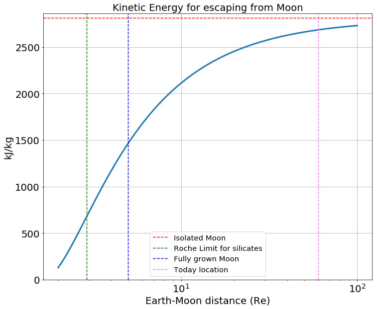
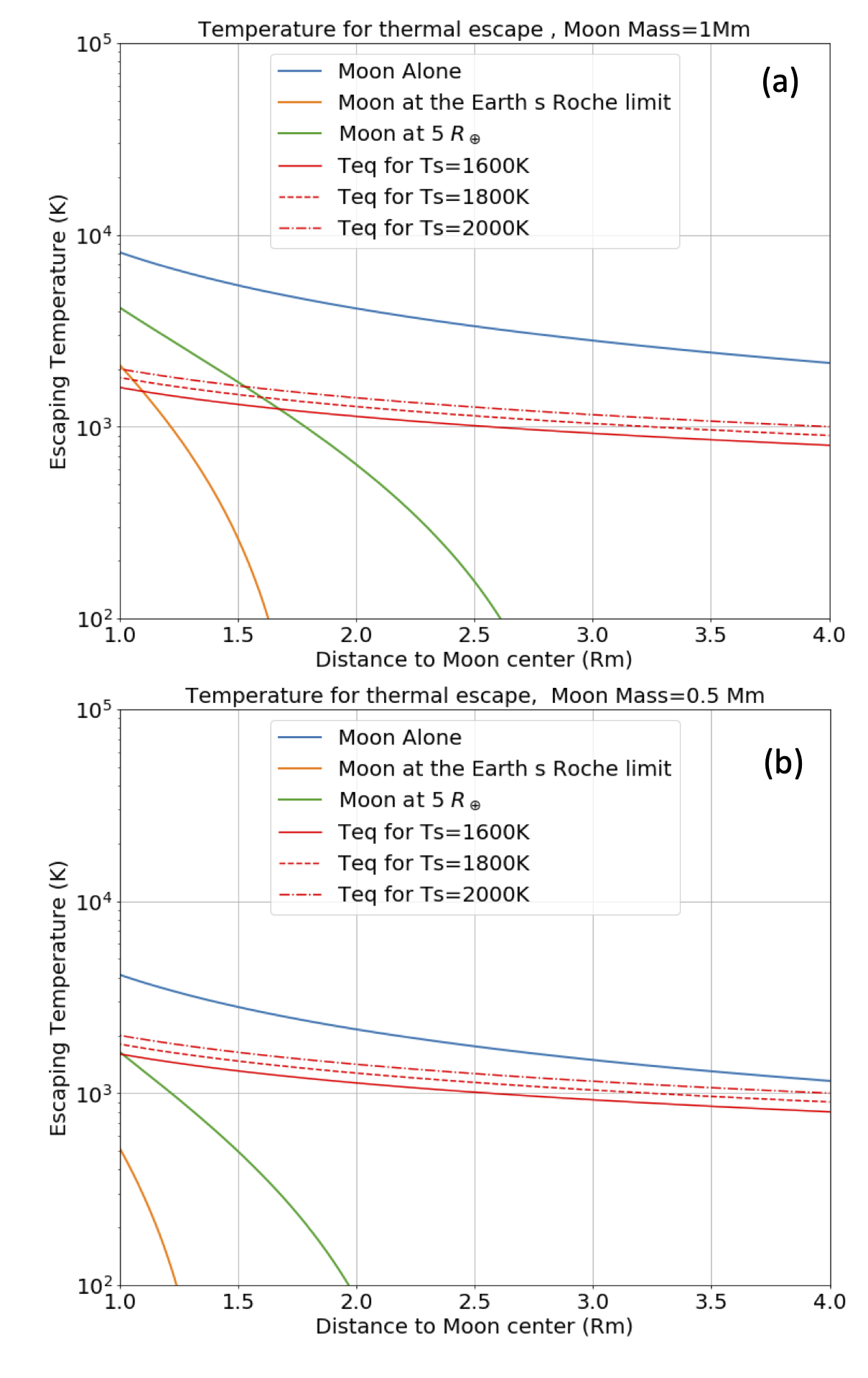
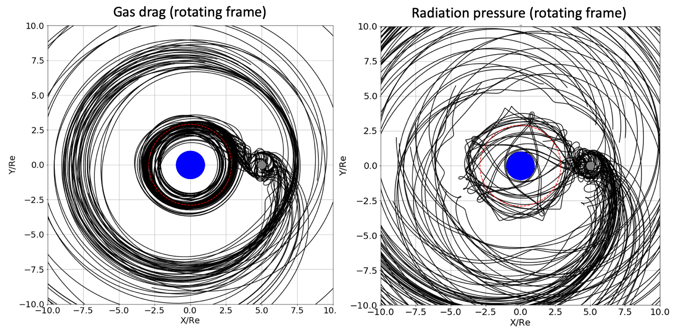
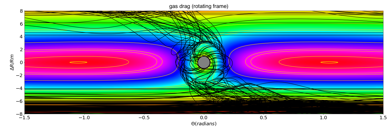
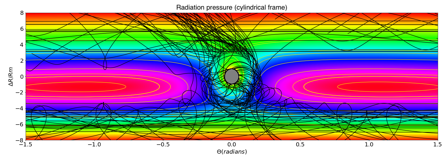
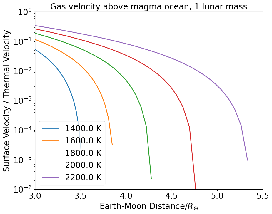
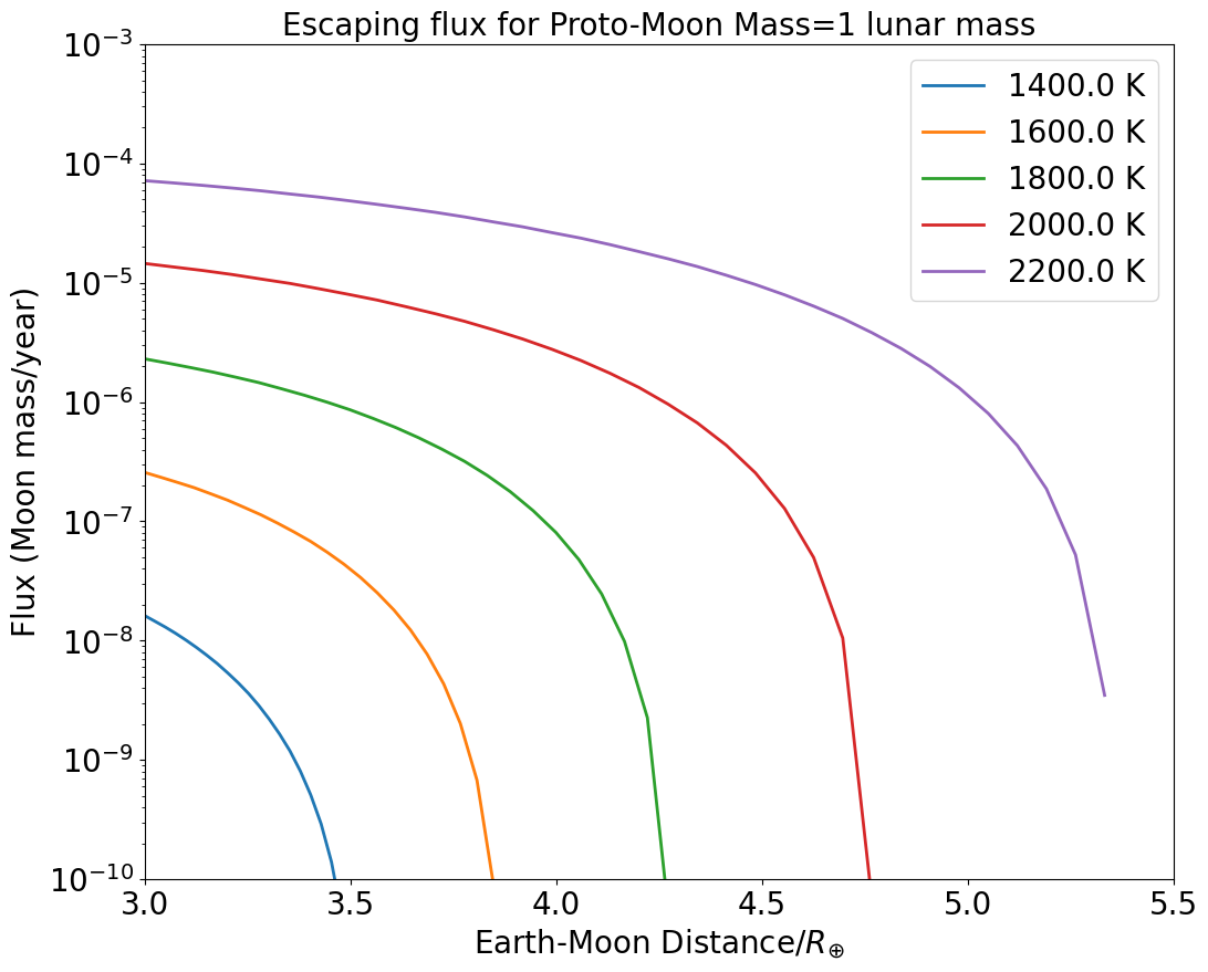
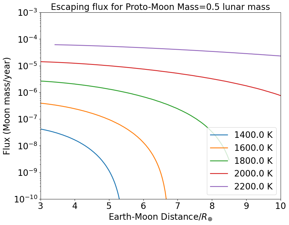
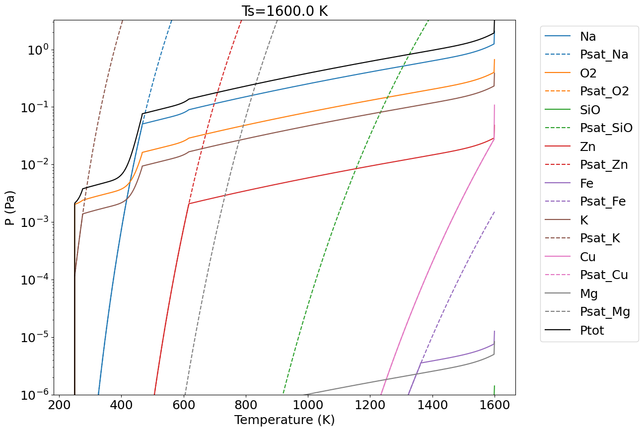
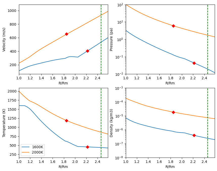
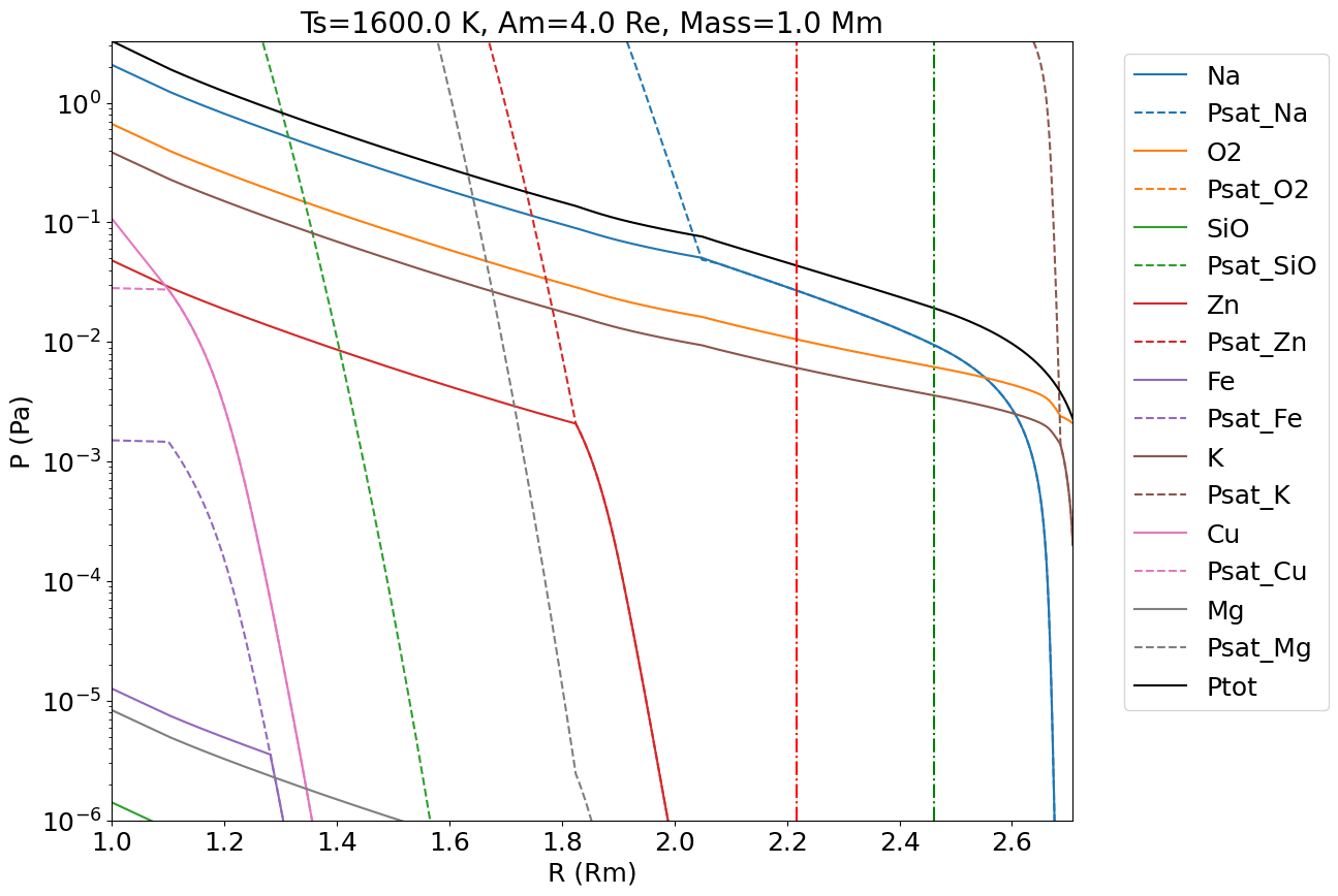
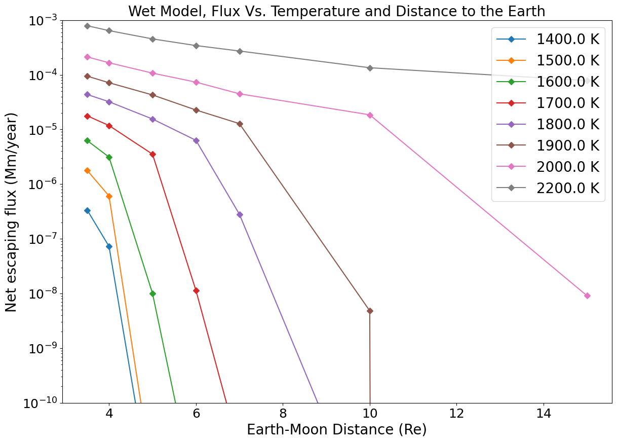
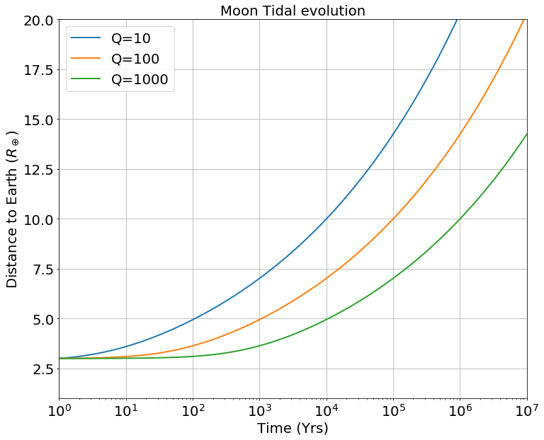
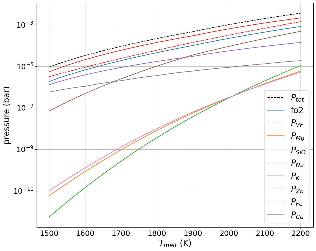
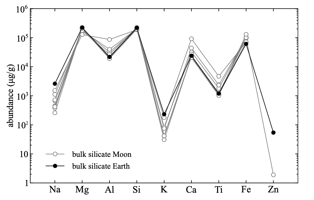
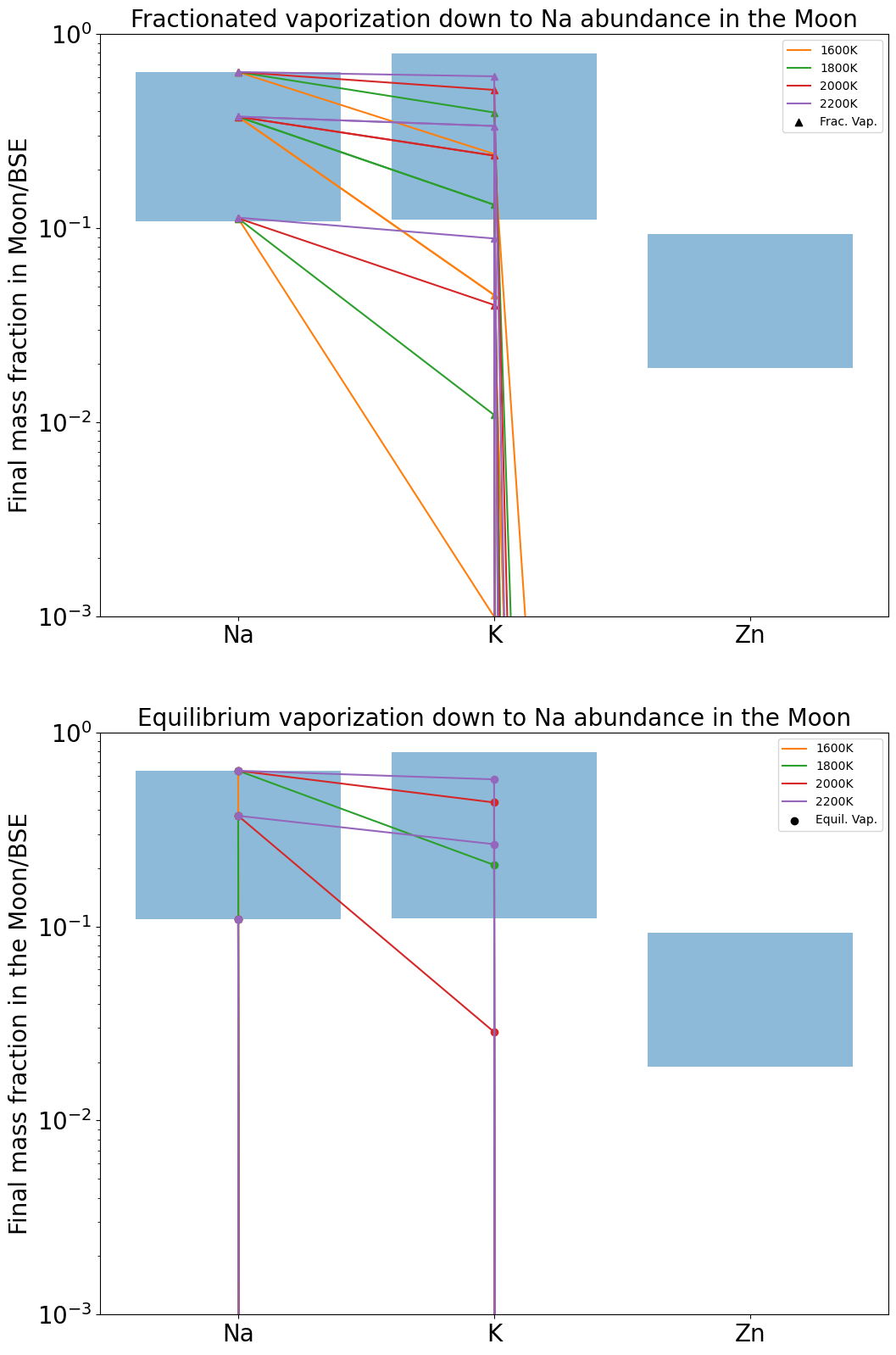
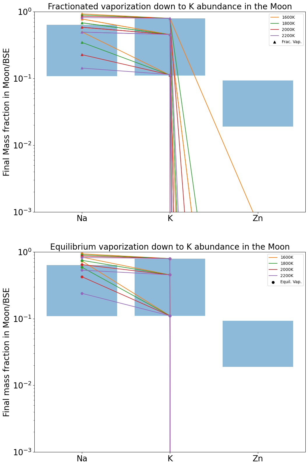
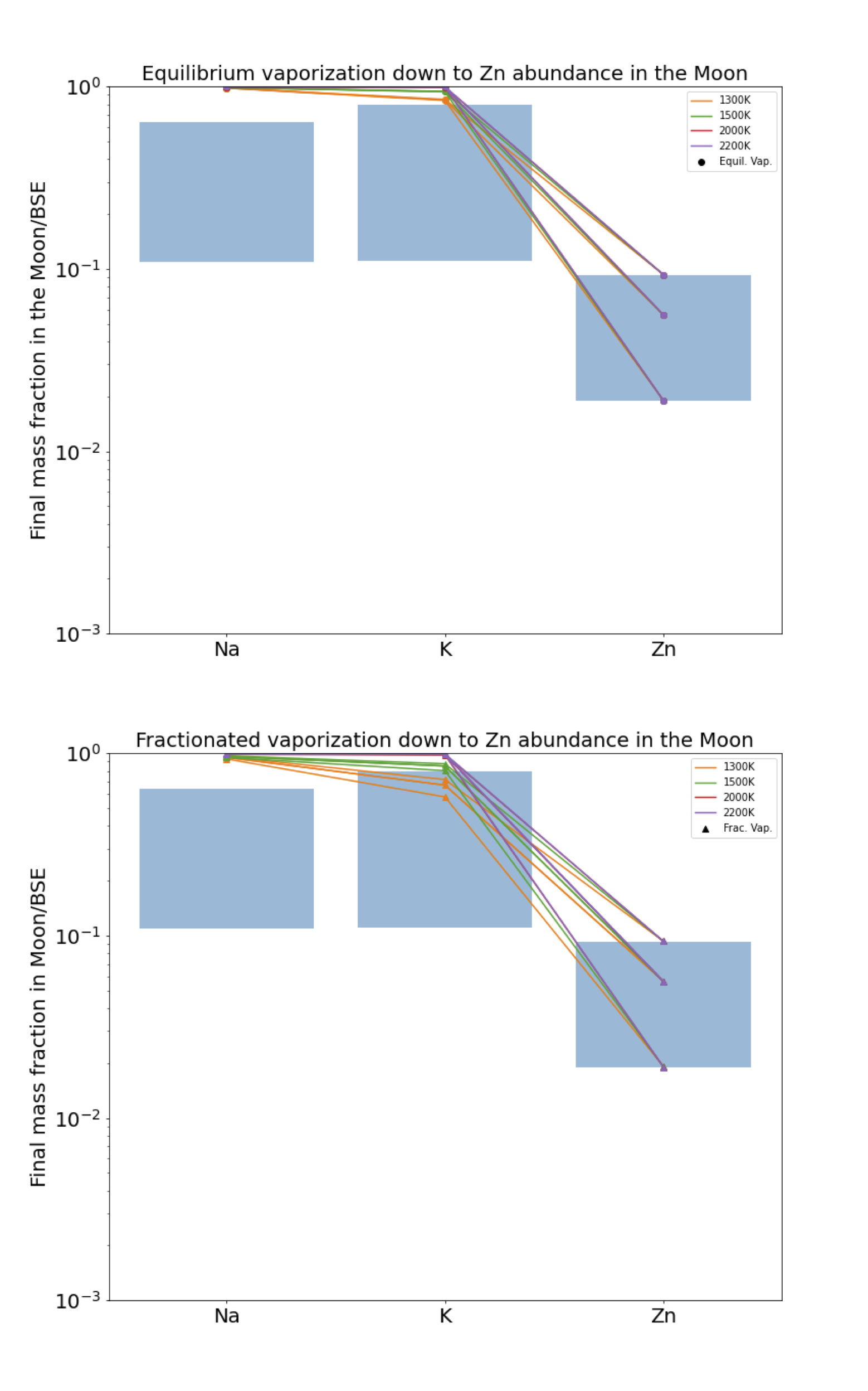
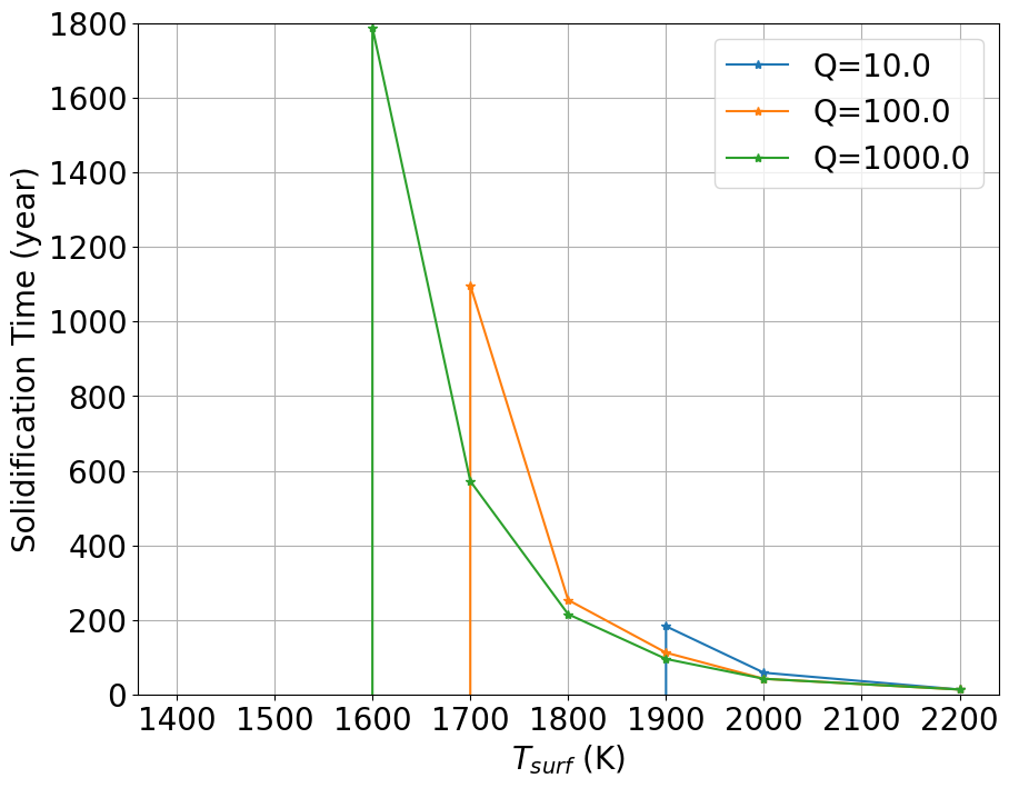
Appendix A Moon gravitational potential in the Earth’s tidal field
We consider a molten Moon located at distance from the Earth, and orbiting on a circular orbit at keplerian frequency :
| (A1) |
With , , and standing for the universal gravitational constant, the Earth’s mass and the Moon’s mass respectively. We work in a rotating frame with axis pointing from the Earth to the Moon, and with origin at the Earth’s center. We compute the acceleration on a line joining the Earth and the Moon. The acceleration felt by a particle is then :
| (A2) |
with is the abscissa of the particle measured from the Moon’s center, is the velocity in the rotating frame and is the rotation vector of the frame. The first two terms are the gravitational accelerations, while the last three terms are the inertial accelerations. The first term corresponds to the Moon’s gravitational attraction, the second is the Earth’s gravitational attraction. The third term is the centrifugal force, the fourth is the opposite of the acceleration on the the center of the system (the Earth) because we work in an accelerated frame. The last term is the Coriolis acceleration, but which has a null contribution onto the axis joining the Earth-Moon’s centers. The corresponding potential energy is :
| (A3) |
where is the projection of the Earth-centered position vector onto the line joining the Earth to the Moon’s center.
Under the Earth tidal field, two potential maxima appear on both sides of the Moon: the L1 and L2 Lagrange points. Their absolute distance to the Moon’s center is given, approximately, by the Hill Radius :
| (A4) |
Note that for the acceleration is directed toward the Moon and for the acceleration is directed opposite to the Moon’s center. So any material bounded to the Moon’s surface must be closer than to the Moon’s center.
Appendix B Radiation pressure around the Earth
In this subsection, we discuss the ratio () of radiation pressure force to gravitational force on a dust grain. The effect of radiation pressure is discussed in a context of Martian moons-forming gas/dust disk [Hyodo et al., 2018] produced by a giant impact on Mars [Hyodo et al., 2017]. Here, following their simple approach, we estimate values of condensed small particles as a function of their sizes and temperature of the Earth. values is given by
| (B1) |
where and are the radiation pressure force and gravitational force respectively. is given by [Burns et al., 1979]
| (B2) |
where is the Plank mean of the radiation pressure efficiency averaged over the spectrum. is the speed of light. is the cross section of a particle whose radius is . is the radiation flux density at distance to the Earth and given by
| (B3) |
where is the Stefan–Boltzmann constant. is black-body temperature of the Earth. Since , the is rewritten as [Hyodo et al., 2018]
| (B4) |
where and are the densities of the Earth and that of a condensed dust, respectively. In order to calculate , we follow a simple approach discussed in the previous work [Hyodo et al., 2018]. is given by
| (B5) |
where is the normalized Planck function at a wavelength of and is the radiation pressure efficiency as a function of where we assume that is unity for particles whose characteristic length is larger than wavelength and zero vice-versa (thus ). Note that, the above equation indicates that the value of does not depend on the radial distance to the central planet.
Figure 20 shows the values around the Earth as a function of particle size. As the temperature of the Earth increases or as the density of particles becomes smaller, the values become larger. The critical value of for a particle whose orbit is circular to be blown-off by radiation pressure is . If a particle orbit is an eccentric orbit, the critical value of depends on radial distance to the central planet and can be larger/smaller than 0.5 [Hyodo et al., 2018]. Figure 20 indicates that if the black-body temperature of the Earth is K and the density of particle is g cm-3, then , which is enough for particles not coming back to the Moon (see Figure 3).
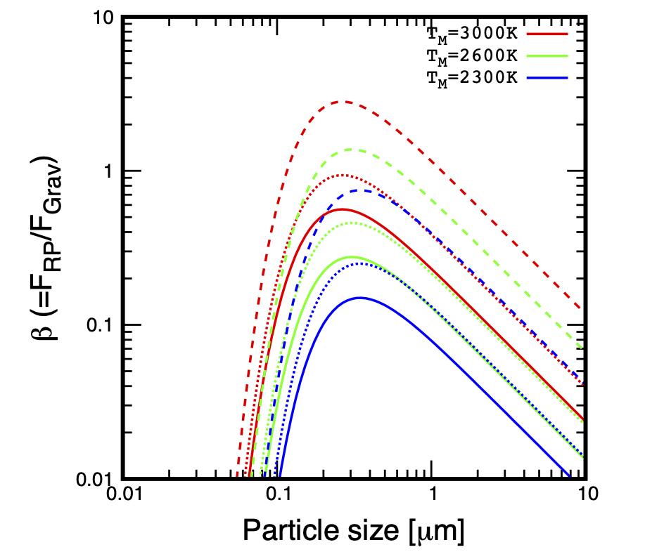
Appendix C Drag of liquid droplets
We have assumed that the droplets stay tightly coupled to the gas. Of course there should be a maximum size above which this assumption must be invalid. The coupling time of a dust-grains with the surrounding gas, is in the Stokes regime[Birnstiel et al., 2011]:
| (C1) |
where is the condensate density (3000 kg/m3 here), is the condensates radius, is the molecular cross section ( with standing for the molecular radius, here m, valid for Na atoms), and is the pure gas sound speed.
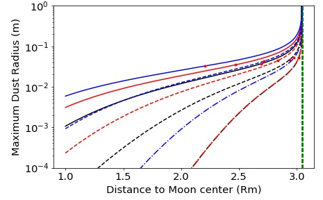
As the droplets are formed in the gas traveling upward, they form keeping an upward directed velocity. During their ascension, they are slowed-down by the Moon gravity field, while being accelerated upward by the friction with the gas. Thus, we compare the slowing-down time due to the gravity field () to the gas coupling time. We define the coupling parameter as follows : . If then condensates stay tightly coupled to the gas, while if the condensates start to fall before they couple to the gas. From condition we can derive a maximum droplet radius for coupling can be derived for every r:
| (C2) |
Finally the Epstein gas-drag regime does not play a role here. As shown on Figure Appendix21 particles are mostly decoupled from the gas at the base of the atmosphere, due to the strong gravitational pull from the Moon and the resulting short acceleration timescale. In this region the gas is dense, so that the Epstein regime does not apply. At the top of the atmosphere, when the gas density drops severely, particles simply follow ballistic trajectories: they are not efficiently decelerated by the Moon’s pull.
Concerning the growth of droplets during their journey upward, it depends on the turbulence state of the flow which is unknown for the moment.
Appendix D What is the net evaporative flux, and pressure, above the magma ocean ?
In Tang and Young [2020] (TY20 hereafter) it is argued that the pressure of the evaporating material above the lunar magma ocean is about bar, far below its saturated vapour pressure ( bar at ). This conclusion is reached by finding the pressure at which the escaping flux at the top of the atmosphere (namely, the point of escape; the Bondi radius) yields an escape rate that can be sustained by diffusive transport of the evaporated material through the atmosphere. These two processes have opposing dependencies on total pressure, in which escape rate increases linearly with pressure, whereas mass transport rates (by diffusion) decrease linearly with pressure. In Figure 6 of TY20 it should be noted that the x-axis is incorrectly designated as the ”surface pressure”, but it actually corresponds to the ”far-field” pressure as introduced in Richter et al. [2002] and re-used in Young et al. [2019]. In TY20 the ”far-field pressure” is also designated as the ”ambient pressure” in their section 3. The concept of far-field pressure was used in Richter et al. [2002] to designate the pressure far (or at infinity) from the surface of an evaporating bead of CAI-like composition, immersed in a surrounding static gas ( in Richter et al., 2002). Inside this static gas, the only mode of mass transfer is diffusion, which proceeds through binary collisions between the evaporating species and the surrounding gas. Indeed Equation 6 of Richter et al. [2002] is simply Fick’s law of mass diffusion, applied to a dilute species (the evaporating gas) diffusing through an ambient medium (a gas, in this case) with a fixed diffusion coefficient that remains constant with distance from the surface. The analytical solution to this equation is reported in Equation 6 of Young et al. [2019] and Equation 4 of Tang and Young [2020]. Richter et al. [2002] shows that at steady-state (), the far-field pressure (as defined above) is lower than the vapour pressure () of the evaporating species at the evaporative surface. As a consequence, the net evaporative flux is lower than the free evaporative flux. This leads Tang and Young [2020] to the conclusion that the net escaping flux is very low. The far-field pressure is found to be about , a pressure at which hydrodynamic escape rates and evaporation rates are found to be equal. However, the use of the Richter et al. (2002)’s approach, is motived by TY20’s assumptions that the escaping flow does not start at the surface of the magma ocean, but starts above a convectived layer, just above the magma ocean. So there is no net advection at the surface of the magma ocean (by hypothesis). In our case the upward advection of the atmosphere starts at the bottom of the atmosphere. So the R02 appraoch is not suited for in our case for the following reasons :
-
•
The evaporating species are not transported in the vertical direction through diffusion alone, but through advection, with a non-zero net upward velocity. The acceleration is provided essentially by the strong pressure gradient between the surface and infinity. In this context, the classical Euler hydrodynamic equations (conservation of mass, momentum and energy as used here) must be considered to describe properly the atmospheric structure, rather than Fick’s law only.
-
•
The evaporating species is not a minor constituent as assumed in Richter et al. (2002), and, again its transport cannot be simply described by diffusive transport: its presence affects the local flow velocity and pressure field, and thereby requires an equation of state (the ideal gas law) to yield a self-consistent solution.
So our description of the connection of the magma ocean in our model and in TY20 model differ largely. For the above reasons, we do not follow the approach of Tang and Young [2020]. In addition, the concept of far-field pressure, whereas properly defined in the context of Richter et al.(2002), becomes ill- defined in our case, because we do not know ”where” to take it. If it is the pressure at infinity (as defined in Richter et al. 2002) , then it should be zero for a Parker Wind, like considered in Tang and Young [2020]. But the Parker Wind do solve for the conservation of mass, momentum and energy fluxes, that is inconsistent with the Richter et al. (2002)’s approach.
However, a point still holds and must be discussed here: Richter et al. [2002], Young et al. [2019] and Tang and Young [2020] argue correctly that there should be a ”return flux” () of evaporating material back to the magma ocean. This return flux is opposed to the free evaporative flux (), and thus the net escaping flux () is the difference between the two. The net evaporative mass flux in a static gas ()is given by the Hertz-Knudsen equation:
| (D1) |
| (D2) |
with and standing for the actual pressure and molar mass of evaporating specie . At thermodynamic equilibrium and so the net escaping flux is zero. However the above equations are not valid for a non-static gas, i.e a gas that is globally advected away from the evaporating surface, like an expanding atmosphere above a magma ocean. Whereas this does not affect the free evaporative flux, the return flux must be reconsidered.
We present here an approach very similar to the original Hertz-Knudsen theory, but generalized to a moving gas to compute the return flux. We show that in a system in which the net advective gas velocity is non-zero, the surface pressure remains comparable to as long as the advective velocity is small compared to the thermal velocity. We proceed as follows: consider a liquid surface located at Z=0 and temperature T. We assume that the gas has a non-zero advective velocity above the surface called and directed upward. This non-zero velocity is due to the atmospheric structure that gives rise to a vertical acceleration due to the pressure gradient, allowing it to escape from the system. The free evaporative mass flux per surface unit may be simply written (replacing pressure by density, using ideal gas equation, in the fluxes equations above):
| (D3) |
where is the gas density at saturation at temperature T ( ) where . is the ”thermal velocity” meaning precisely the most problable velocity in the Maxwell Boltzman velocity distribution . Let the return flux to the melt. We assume also the gas density at the surface, , is unknown. We can write, in a general way that:
| (D4) |
where has the dimension of a velocity, and can be seen also as the flux of particles returning back to the liquid, in gas unit volume above the surface. For a static gas, for example in a closed system and equation 3 of TY20 is recovered. However, for an atmosphere in motion, we require the general expression of . Consider a parcel of gas above the liquid, at a few particles mean-free path above the surface. There, the velocity distribution of particles follows a Maxwell-Boltzmann distribution at temperature T but with a non-zero net-vertical velocity with . So in the reference frame of the liquid’s surface the 3D velocity distribution of gas particles is not centered on the velocity vector (as in a static gas), but rather centered on , because the evaporating gas is globally accelerated upward in this open system. The particle 3D velocity distribution is then :
| (D5) |
where is the decentered Maxwell Boltzmann velocity distribution :
| (D6) |
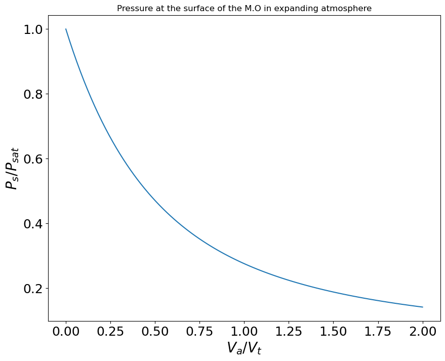
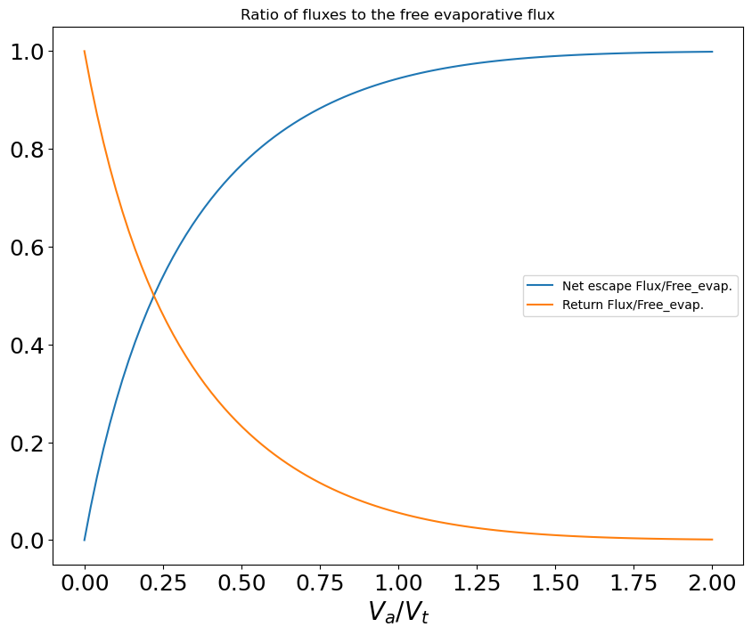
Then can be computed : it is the flux of particles crossing the surface, that is the flux of particles with (in the reference frame of the liquid surface). Counting the flux positively for particles with , so which gives :
| (D7) |
And we get, after integration :
| (D8) |
where is the complementary error-function (). So the net return flux is :
| (D9) |
Which we rewrite for easy manipulation
| (D10) |
With C(x) :
| (D11) |
Note that in the limit case of a static gas (like in a closed chamber) and we recover the return flux as reported in Richter et al. [2002], Young et al. [2019], Tang and Young [2020] valid for a static-vapour. The gas density (and pressure) above the surface is obtained by considering mass conservation. The relation between the escape-flux (), the free evaporative and return flux is : that reads :
| (D12) |
Thus
| (D13) |
or
| (D14) |
Since we assume that the liquid and the gas are at the same temperature at the surface . is plotted in Figure 22 as function of . It shows that for the surface pressure is equal to the saturating vapor pressure. For the surface pressure diminishes slowly, which allows a net and non-zero escaping flux. When the advective velocity (and the net escaping flux) increases, the surface pressure may drop significantly. For our present paper we find surface velocities that are in the range (for magma ocean at 2200 K and for a Moon orbiting at 3.5 Earth radii only) so that is comparable, but still lower, than the saturating vapor pressure. So liquid-vapor equilibrium is almost reached at the surface of the magma ocean and in no-way is the surface pressure as low as , nor is it this low at the escaping Bondi radius. The origin of this discrepancy is due to the reliance on diffusion in TY20 as the dominant mode of mass transport.
For the sake of completeness we provide below the useful quantities, and
| (D15) |
| (D16) |
They are plotted in Figure 23 .
Appendix E Isothermal models
In the core section of the text we have assumed that escape was always adiabatic. As the gas pressure is quite low (¡ 100 Pa at the base of the atmosphere), a thin and transparent atmosphere may indeed behave adiabatically. However, as gas condense into droplets, the optical depth may increase, leading to stronger absorption. So it is also interesting to present isothermal solutions for the hydrodynamical escape.
For the dry model (without recondensation), we now have and the isothermal Bernouillie relation is rewritten :
| (E1) |
The resulting flux is displayed in Figure 24.
For the wet model, following the procedure described in the core text (see section 3.2), we have recomputed the fluxes, but only keeping the isothermal part, keeping . The isothermal wet fluxes are displayed in Figure 25. In bothe cases we see that the isothermal fluxes drops slowly with distance. This can be understood by examining Equation E1 where the dependency on is logarithmic in the isothermal case. So almost do not play a role during the escape. As a results only balances the variation of potential energy , which varies only by a factor of 3 between 3.5 and 10 Earth radii (see Figure 1). In consequence V, as well as the flux, varies only by a factor between 3.5 and 10 Earth radii. This corresponds approximately to what is observed in Figures 24 and 25.
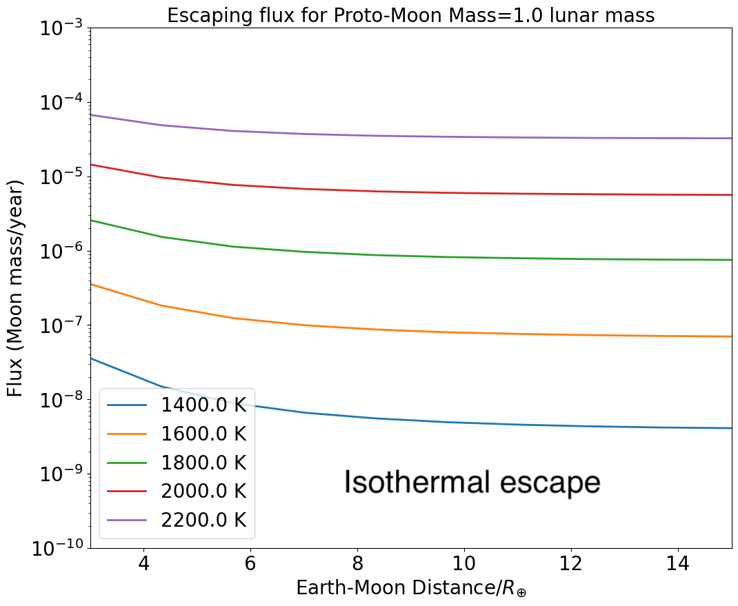
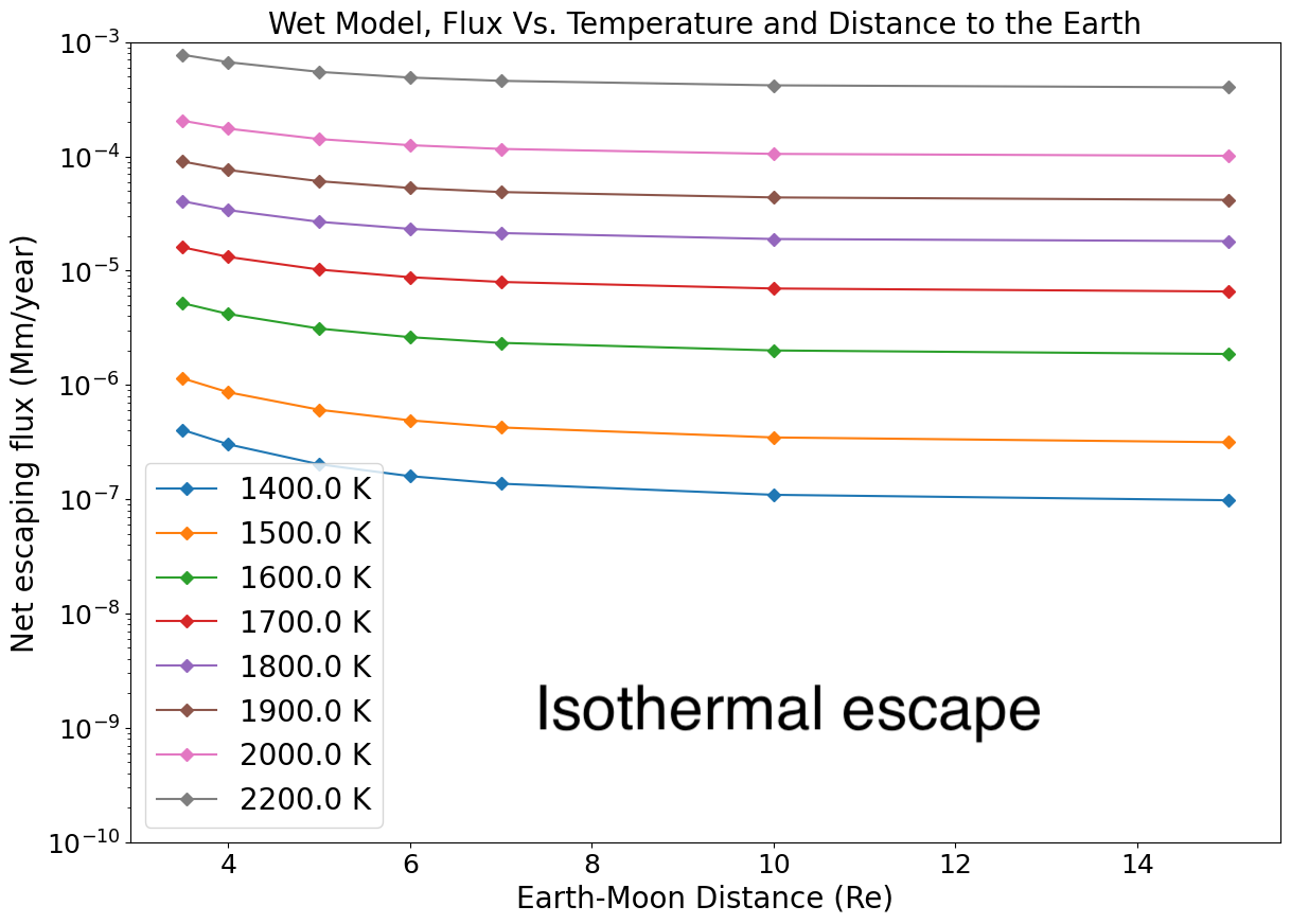
Appendix F Renewing of the magma ocean material through convection
In the model described above the magma ocean is simply considered as a ”source” function, that provides gas to the atmosphere at that maintains the base of the escaping atmosphere at constant temperature, , and ensuring thermodynamical equilibrium of the gas with the liquid. It was also assumed that the magma droplets dragged by the gas have a BSE composition. This implies that during the degassing, there is a constant renewing of the magma surface material, rapid enough to maintain its surface with BSE composition, despite of the enrichment in refractory material due to degassing. We now estimate the typical timescale of such a renewing.
When the magma ocean is fully-liquid, it convects vigorously, in a turbulent regime. The convective heat flux that escapes from this turbulent magma ocean scales as [Kraichnan, 1962, Siggia, 1994]
| (F1) |
where
| (F2) |
is the Rayleigh number, is the thermal conductivity, the temperature difference across the magma ocean, the magma ocean depth, is the thermal expansion coefficient, the gravity at the Moon surface, the thermal diffusivity, the kinematic viscosity. Using K-1, ms-1 and ms-1 for fully-liquid silicates [Bottinga et al., 1983, Karki and Stixrude, 2010, Eriksson et al., 2003], and m2s-1 at the Moon surface, km close to the Moon radius, and in the range K [Solomatov, 2000], we obtain and in the range J ms-1.
The velocity for turbulent convection scales as [Kraichnan, 1962]
| (F3) |
where is the heat flux from the ocean to the atmosphere, the thermal capacity of liquid silicates, the magma ocean density. Using the above estimate for , and assuming kg m-3 for the Moon and J kgK-1 [Solomatov, 2000], we find convective velocities m s-1. The associated turnover time scale in the magma ocean is days. This implies that the silicates below the Moon surface are renewed in about days.
Appendix G Silicate volume brought to the surface
Assuming volatiles exsolve from the magma ocean as gas bubbles [Hamano et al., 2013, Salvador et al., 2017], the volume of liquid silicates that can interact with the atmosphere, before the magma ocean solidifies at time , is
| (G1) |
where is the Moon radius. Assuming a solidification time ranges from years[Tang and Young, 2020] to yrs[Solomatov, 2000], we obtain
| (G2) |
where is the Moon volume. In this case, is orders of magnitude larger than the volume of the Moon. Hence, the whole magma ocean has time to interact with the atmosphere. We therefore expect that including the dynamics of the magma ocean will not affect the leading-order conclusions of this paper.
Appendix H Location of the photosphere
We have computed the atmospheric optical depth assuming that liquid droplets are the only source of opacity. The droplet radius, is a fixed parameter and the droplets density is . With these assumptions the optical depth, integrated from the Hill Sphere down to some distance from the Moon’s center, r, is :
| (H1) |
where is the Hill sphere location, is the density of the liquid-gas mixture and is the droplet mass fraction. We define the photosphere as the location where . We take . Results are presented for different Earth-Moon distances and for different droplet radii : 0.01 mm (Figure 26) and 1 mm (Figure 27). As expected, for larger particle size the photosphere is closer to the ground (i.e. the atmosphere is more transparent), and for a larger Earth-Moon distance also. Interestingly the temperature is the main parameter controlling the location of the photosphere. We find that the transition from an opaque atmosphere (with ) to a transparent atmosphere ( ) occurs for temperature between 1800 K and 2400 K for an Earth-Moon distance = .
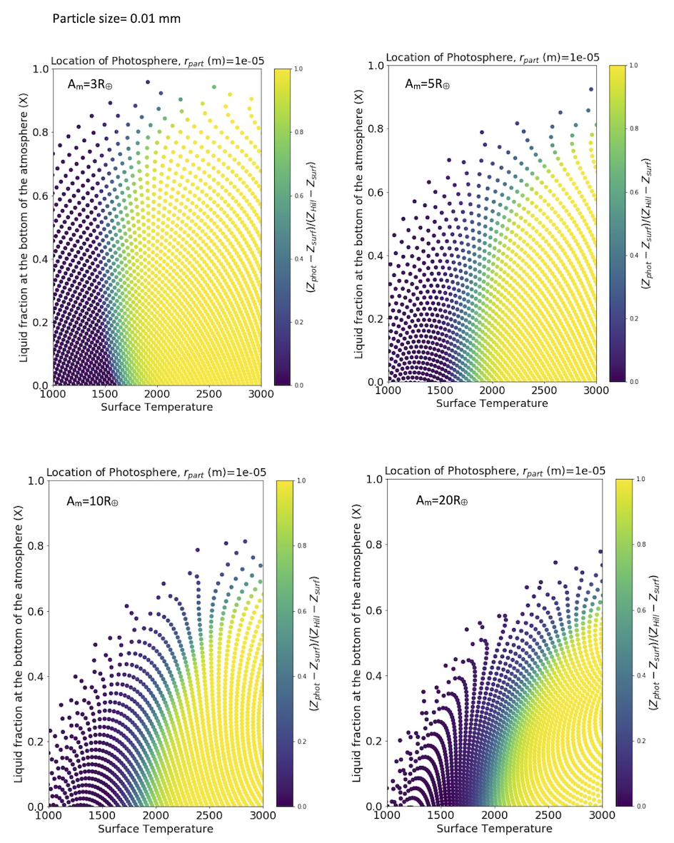
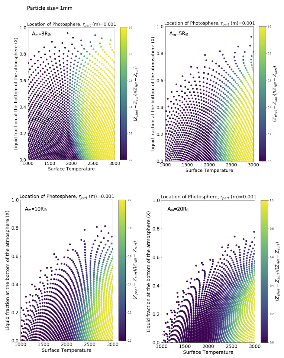
Appendix I Composition of the vapor atmosphere
The saturated vapor composition of an atmosphere at equilibrium with a magma with BSE composition was recently published [Visscher and Fegley, 2013]. However this work does not extend below 2000 K, a temperature regime of interest to explain the Moon composition. Using up to date thermodynamic data(Sossi and Fegley Jr. [2018]), we have computed the vapor composition for K. The equilibrium partial pressure may be calculated for any given vaporisation reaction:
| (I1) |
where denotes the liquid phase, the gas phase, the oxidation state of the metal in the gas phase and the coefficient of stoichiometry (an integer value). We note the equilibrium constant of this reaction. From Equation I1 the equilibrium partial vapor pressure of species (designated as species for short) is obtained as follows :
| (I2) |
where is the mole fraction of species (see table below), its activity coefficient and the oxygen fugacity.
Here we estimate the activity coefficients of Na, K, Cu and Zn based on thermodynamic measurements from laboratory experiments on basaltic melts (Na, De Maria et al. 1971, Mathieu et al. 2008 and Sossi et al. 2019; K, De Maria et al. 1971, Hastie et al. 1983 and Sossi et al. 2019; Cu, Sossi et al. 2019, and Zn, Reyes and Gaskell, 1983 and Sossi et al. 2019). The ratio / is set to remain constant as a function of temperature (cf. Charles, 1967) where is taken to be at 1700 K and at the same temperature. Uncertainties in these values are as large as a factor of 5, see also Jiang et al. (2019). For example, Mathieu et al. 2008 provide a value of = at 1623 K, Sossi et al. (2019) report the same value at 1673 K, whereas the Knudsen Effusion Mass Spectrometry measurements of De Maria et al. (1971) suggest a of at 1500 K. Copper may exist in its 2+ and 1+ oxidation states in silicate melts (Holzheid and Lodders, 2001), however at the oxygen fugacities produced by evaporation of the lunar silicate ( FMQ), it occurs uniquely as . We assume that the major element oxides (, and ) dissolve ideally into silicate melts (e.g. O’Neill and Eggins, 2002; Beckett, 2002).
Here, we take the model of Visscher and Fegley (2013) as an input parameter to calculate . This model compares well with measurements of oxygen fugacities above vaporising silicates above 1400 K (see Fig. 4 of ref. Sossi and Fegley Jr. [2018]). The values of , the stoichiometric coefficient of the vaporisation reaction, is an integer value equal to 1 (Na, K) and 2 (Mg, Fe, Si, Zn). As such, the condensed species considered are: , , , , , and , all (l) and the gas species are: , , , , , , and . We consider only these eight elements as they have the most abundant species in the vapour ¡2000 K [Visscher and Fegley, 2013].
Following our experimental data of BSE vaporisation we use the values for reported in Table 4.
| Temperature (K) | 1500 | 1600 | 1700 | 1800 | 1900 | 2000 |
|---|---|---|---|---|---|---|
| (bar) |
Here are the thermodynamic parameters for the different species of interest. The molar abundances :
| Species | X (Mole Fraction) |
|---|---|
| Na | |
| K | |
| Cu | |
| Zn | |
| Mg | |
| Fe | |
| Si |
In order to predict the temperature dependence of the activity coefficients of Na, K and Zn in silicate melts, we draw upon pre-existing experimental data. Charles (1967) determined the activity coefficients of and in alkali oxide - binary systems by application of the cryoscopic equation to pre-existing vaporisation data, thereby determining heats of solution of oxide components in the silicate melt. The two quantities are related by the van’t Hoff equation:
| (I3) |
We take values of from Charles, 1967 for (-112 kJ/mol) and fix as , while we use the values determined by Reyes and Gaskell (1983), -135 kJ/mol and Sossi et al. (2019), -143 kJ/mol for ZnO, with 121 kJ/mol for from Sossi et al. (2019). All quantities are extracted presuming infinite dilution of the trace component in the silicate melt.
The estimated activity coefficients are therefore the following :
| Temperature (K) | 1500 | 1600 | 1700 | 1800 | 1900 | 2000 |
|---|---|---|---|---|---|---|
| for | 0.0004 | 0.0008 | 0.001 | 0.002 | 0.003 | 0.004 |
| for | 0.0002 | 0.0004 | 0.0005 | 0.001 | 0.0015 | 0.002 |
| for | 37.6 | 20.5 | 12 | 7.5 | 4.9 | 3.3 |
| for | 0.18 | 0.42 | 0.56 | 0.65 | 0.71 | 0.75 |
The equilibrium constant may be calculated using thermodynamic data (e.g. Chase 1998) using the expression:
| (I4) |
in which
| (I5) |
We use the following enthalpies and entropies :
-
•
J/mol (Lamoreaux and Hildenbrand, 1984)
-
•
J/mol(Lamoreaux and Hildenbrand, 1984)
-
•
J/mol (Lamoreaux et al., 1987)
-
•
J/mol (O’Neill and Pownceby, 1993)
-
•
J/mol (Chase, 1998)
-
•
J/mol (Chase, 1998)
-
•
J/mol (Chase, 1998)
The resulting partial pressure are plotted in Figure 14.
Appendix J Caveats and approximations
This paper aims to show that degassing during the lunar assembling is potentially an important process, and may explain the depletion of lunar material in moderately volatile elements. Of course, to make the computation tractable, several approximations must be done, and before making a fully self-consistent model we aim here to show that first-orders calculation show that tidally driven evaporation is a viable process. Our simplifications are summarized below:
-
•
Radiative heating and cooling : The present work does not consider radiative heating and cooling processes that may act during the gas expansion. Only adiabatic cooling is considered. This would require to couple the dynamical model to radiative transfer code, that has never been developed for an atmosphere expanding above a magma ocean. Computation of the radiative diffusion timescale following Tremblin et al. (equation 17) shows that in the optically thick case the radiative diffusion timescale is shorter than the expansion timescale (a few 10s compared to a few s for droplets in the range of micrometer size), assuming the source of opacity are the droplets in the flow. This implies that the thermal radiation may potentially modify the temperature during the expansion if important temperature gradient is present. In the absence of a full radiative transfer model, we compare two length scales : the temperature scale height ():
(J1) and the photon mean free path (:
(J2) where is the local opacity (computed with assuming that the opacity source is the presence or droplets with a fixed radius). If , this means that a photon experiences several scattering events before reaching a region with significantly different temperature. The assumption of local thermal equilibrium (LTE) is therefore valid, and we do not need to consider the energy loss due to radiation. In the opposite case, the photons can escape without being absorbed and radiative cooling effect should not be neglected. We plot in Figure 28 the ratio between the two length scales for different atmospheric profiles, and being evaluated at the sonic point. We find that at high temperature and at low temperature , the transition between the two regimes situating at K for 1 micron radius droplets and K for 1 mm radius droplets. We conclude that above such temperature, the present work neglecting radiative cooling effects stays valid, whereas at lower temperature complete radiative modeling should be considered.
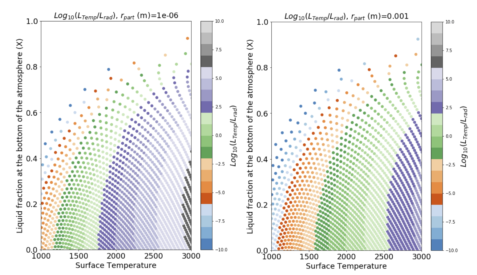
Figure 28: evaluated at the sonic point for a Moon at 5 as a function of the surface temperature and the liquid mass fraction (X). Left : for liquid droplets size=1 micron; Right:for liquid droplets size=1mm. Taking into account radiative cooling and heating from the Moon surface would require to develop a radiative transfer model, well beyond the scope of the paper that intends to identify a new escaping process and to point out its potential importance. However, for the simple case of a collisionless gas, with no pressure and at thermal equilibrium with the hot radiating Moon’s surface, we show in Figure 2.a that the gas temperature becomes always larger than the necessary temperature for escaping for a Moon within 5 of the Earth center’.
This shows that escape is an unavoidable process for a fully grown Moon. Escape becomes even more intense for a Moon’s building block, with a fraction of a lunar mass (Figure 2.b, and core text).
-
•
1D calculation : In this paper we have done the calculation in 1D, along the line joining the center of the Earth and the center of the Moon. So, strictly speaking, the computed flow would be only valid along this line, and it cannot be assumed that the flow is emitted at steradians on the surface. It is why, for simplicity purpose we have assume that the flow is arbitrarily emitted on a solid angle of 1 steradian. The full calculation would need a full 3D treatment, as the gas will probably circulate around the Moon before escaping. But such model is still beyond the state of the art, but could be done in a close future.
Appendix K Lost mass fractions
Let and the Moon and Earth Mass respectively today. Let the mass fraction of an element in the BSE, the mass fraction of an element in the Moon today, and the mass fraction of an element in the vapor at some temperature. We call the total mass lost during degassing of the Moon. where is the mass lost in the form of gas, and is the mass lost in the form of droplets dragged by the gas. We call the total mass of an element in the Moon today and the total mass of an element in the BSE. We assume that the Moon is degassed at constant temperature for simplicity so that is a constant for every species. The Initial mass of the Moon is and final mass is . If we assume that the Moon material was initially BSE composition we have :
(K1) The first term is the initial mass of element the second term is the mass lost in vapor form, and the third term is the mass lost in liquid form (assumed to have BSE composition). Since and ; we get
(K2) Dividing by , the Moon mass, we obtain
(K3) (K4) In the above equation the effect of degassing on the mass fraction in the Moon () is obvious. No degassing means so stays equal to the BSE value . if (which is the case for volatile species in general) then degassing lowers the value of .
From Equation K4 we derive the mass fraction of an element remaining in the Moon, compared to its mass fraction in the BSE:
(K5) From the above equation we see that fractionation, compared to the BSE, is only possible through vapor loss. If then this element will be enriched in the Moon, conversely elements with will be depleted in the Moon.
Appendix L Enhancement of Volatile Loss due to XUV Heating from the Proto-Earth
While our model treats tidally-driven escape heated uniquely from the bottom by the magma ocean, additional heating from the top by XUV irradiation as at exoplanets [Erkaev et al., 2007] and even Kuiper Belt Objects [Johnson et al., 2015] gives further credence to the Moon’s devolatilization by atmospheric escape. By employing the atmospheric evolution model DISHOOM [Gebek and Oza, 2020] we investigate mass loss due to surface and upper atmospheric heating. We find that while the tenuous Jeans escape rates due to surface heating are quite small, catastrophic volatile loss ( Myr) must still occur due to a remarkably bright proto-earth[Saxena et al., 2017] heating the upper atmosphere via XUV energy-limited escape. Figure 29 shows three scenarios of three different estimates of the proto-Earth temperature with distance. We adopt a heating efficiency of 0.35 similar to Io’s volcanic atmosphere[Lellouch et al., 1992]. A conservative assumption, neglecting atmospheric sputtering, that the only proto-earth irradiation driving escape is due to the X-ray and UV component () still yields a total mass loss of of a lunar mass, in 1 Myr. The mass loss rates on the order of kg/s are then quite similar to an early magma-ocean planet at 1 AU orbiting an M-dwarf[Bower et al., 2019] or a close-in exomoon[Oza et al., 2019]. Considering the timescales and proximities studied in this work, a catastrophic volatile loss scenario for the Moon seems inevitable.
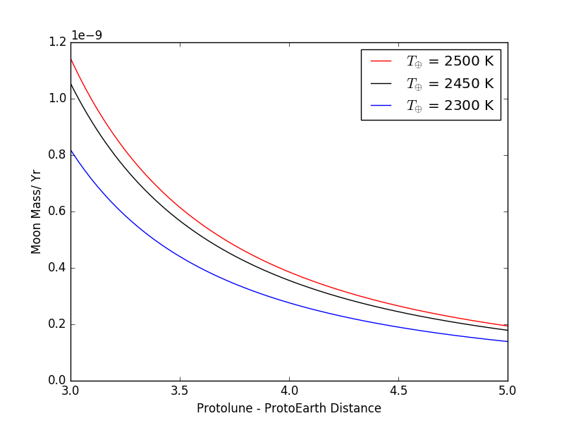
Figure 29: Energy-limited escape from the proto-Moon due to irradiation of a molten proto-Earth at three different effective temperatures : 2500 K (red), 2450 K (black), 2300 K (blue).