Tight-binding model with sublattice-asymmetric spin-orbit coupling
for square-net nodal line Dirac semimetals
Abstract
We study a 4-orbital tight-binding (TB) model for ZrSiS from the square sublattice generated by the Si atoms. After studying three other alternatives, we endow such model with a new effective spin-orbit coupling (SOC) consistent with ab initio dispersions around the Fermi energy () in four systematic steps: (1) We calculate the electronic dispersion of bulk ZrSiS using an implementation of density-functional theory (DFT) based on numeric atomic orbitals [J. Phys.: Condens. Matter 14, 2745 (2002)] in which on-site and off-site SOC can be told apart. As a result, we determine that local SOC-induced band gaps around are predominantly created by the on-site contribution. (2) Gradually reducing the atomic basis set size, we then create an electronic band structure with 16 orbitals per unit cell (u.c.) which retains the qualitative features of the dispersion around , including SOC-induced band gaps. (3) Zr is the heaviest element on this compound and it has a non-negligible contribution to the electronic dispersion around ; we show that it provides the strongest contribution to the SOC-induced band gap. (4) Using Löwdin partitioning approach, we project the effect of SOC onto the 4-orbital Hamiltonian. This way, we facilitate an effective SOC interaction that was explicitly informed by ab initio input.
I Introduction
Topological semimetals (TSMs) are a class of materials whose crossings between valence and conduction bands are topologically protected [1]. There are two main subcategories of TSMs: nodal point semimetals (NPSs), and nodal line semimetals (NLSs). NPSs have a discrete set of crossing points at , while NLSs display a continuous crossing line. Initial, theory-lead searches for NLSs called for materials with nonsymmorphic symmetry [2, 3] such as ZrSiS [4], ZrSiSe, and ZrSiTe [5]. Those materials display unusually-high magnetoresistance [6, 7, 8, 9, 10], high carrier mobilities [11, 7, 12], and linear band dispersions around [4, 6, 13].
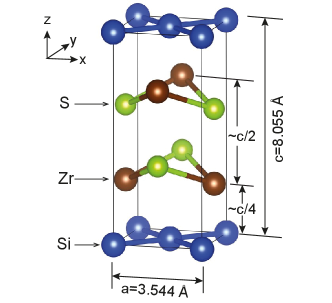
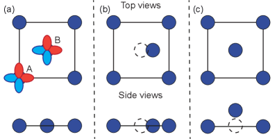
ZrSiX (X=S, Se, or Te) belongs to the nonsymmorphic P4/nmm space group. As shown in Fig. 1, two atoms of each species are present in their u.c., with their Si atoms arranged in stacked square nets [14, 15, 16, 17, 18, 19, 20]. The electronic structure of two-site square lattices is described by and orbitals in various models. Indeed, such a basis set was proposed by Luo and Xiang to study a Bi-based topological insulator [21]. Later, Klemenz and coworkers discovered nodal line semimetals in square nets [22, 23, 24], which are 2D symmorphic lattices, and presented a symmetry analysis of such nets relying on and orbitals in Ref. [24] (Fig. 2(a)). Since then, other two additional teams have implemented two-site models to study the effect of SOC in similar nets [25, 26].
Recent quantum oscillation experiments have shown that the Berry phase generated for ZrSiS depends on the orientation of the magnetic field [8, 9] and Yang et al. suggested that a key agent in such dependence is SOC [27]. It is natural to include SOC in models to understand the observations made in Ref. [27]. It is not possible, nevertheless, to gap the crossings at the Fermi level in these models upon the customary implementation of SOC [28]. Luo and Xiang [21], Deng et al. [25], and Aryal et al. [26] independently realized that square net models can be gapped at zero energy through a combination of (i) an on-site SOC (this is, one in which neighboring atoms do not contribute to SOC), and (ii) a lowering of symmetry such that the two atoms in the u.c. turn inequivalent. Such asymmetry was created by a relative displacement of one atom along the 2D plane (Fig 2(b)) [25], or by an out-of-plane relative displacement (buckling, Fig 2(c)) [21]. On the other hand, Aryal et al. incorporated an on-site asymmetry between sublattices directly onto the SOC interaction ad hoc (meaning that no microscopic justification was offered to motivate their choice for SOC interaction).
Given that the Si square nets on ZrSiS, ZrSiSe, and ZrSiTe are in fact not distorted in the way done in Refs. [21] and [25], and that Aryal’s work did not provide justification for their SOC, we seek the source of an asymmetric SOC that could be added to the models to produce a band gap at zero energy, and thus make it consistent with ab initio results containing SOC. The search for that mechanism from ab initio information is our guiding principle, and the motivation for this work.
We have previously worked with 2D models for topological insulators relying on and orbitals also [29], and we possess a deep knowledge of ab initio-informed TB formulations [30] as provided in the SIESTA code [31, 32]. We have written extensions to this code for quantum transport [33] and ab initio molecular dynamics [34] calculations. We are also closely familiar with SOC on this code, down to implementing it [35, 36, 37, 38]. Our knowledge of TB models [39, 40, 41] makes the extraction of TB parameters [42] from SIESTA possible, to the point of turning on-site SOC interactions for analysis at will. This experience underpins the description of a SOC-induced mechanism to break sublattice symmetry.
The article is organized as follows: Sec. II contains a brief overview of the models, and three previous implementations of SOC on them. We demonstrate that the leading contribution of SOC on ZrSiS is due to on-site interactions in Sec. III. To simplify the model, an on-site SOC will be used from that point onwards. A DFT-based TB model is developed in Sec IV by a gradual removal of numerical atomic orbitals from the basis set; we determine the orbitals that contribute to the electronic dispersion of the material around the most, while preserving the SOC band gaps. We also determine Zr to contribute to the on-site SOC the most. Applying the Löwdin partitioning scheme to this auxiliary TB model, we effectively induce SOC-gaps into the model provided in Ref. [24] that break sublattice symmetry in Sec. V. Conclusions are presented in Sec. VI.
II models
II.1 Band folding in models
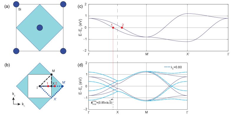
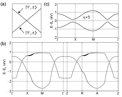
The u.c. of models is represented by the 2D square net depicted in Figs. 2(a) and 3(a), formed by one atom at the corner (A) and another at the center (B). The equivalence among A and B sublattices permits an analysis of the models within the single-atom u.c. (shaded blue square in Fig. 3(a)). Fig. 3(b) depicts the first Brillouin zones associated to the two u.c.s. The first Brillouin zone of the two-atom u.c. (white square in Fig. 3(b)) is related to the first Brilluoin zone of the single atom u.c. (shaded blue square) by folding. Here, primed points () refer to the unfolded Brillouin zone, while unprimed points () describe high symmetry points on the folded Brillouin zone. An exception is the point, which is the same for both, and left unprimed for that reason.
Comparison of the unfolded and folded first Brillouin zones in Fig. 3(b) shows the equivalence among the and points, the folding of the point onto the point, and the fact that the point of the folded Brillouin zone sits halfway among the and points of the unfolded one. We next analyze the consequences of previous observations on the electronic dispersion within the models.
The electronic dispersion within the single-atom u.c. is given by the matrix:
| (1) |
where . This Hamiltonian matrix is written in the basis of rotated orbitals (, and ). Table 1 contains the values of the TB parameters , , and , adapted from Refs. [21, 24, 25, 26]. This electronic dispersion contains two bands (or four when spin degeneracy is considered) and it is shown in Fig. 3(c), where the parameters from Ref. [24] have been used.
| Model | |||||||
|---|---|---|---|---|---|---|---|
| Klemenz et al. [24] | 0.50 | 0.10 | 0.05 | 0.05 | – | – | – |
| Aryal et al. [26] | 1.90 | 0.50 | 0.10 | 0.10 | 0.20 | 0.10 | – |
| Luo et al. [21] | 1.00 | 0.20 | 0.00 | 0.00 | 1.20 | 0.40 | - |
| Deng et al. [25] | 2.00 | 0.70 | 0.40 | 0.14 | 0.02 | – | 0.10 |
The band structure in the 2-atom u.c. is constructed on a basis of four orbitals: , , , , where and label the two sites within the u.c. In this basis, the general form of the matrix Hamiltonian is
| (2) |
where:
| and | ||||
| (3) |
Increasing the size of the u.c. decreases the size of its first Brillouin zone by the same proportion (Fig. 3(b)). This implies that, for every band within the original 2D Brillouin zone, there are two bands in the folded one. Fig. 3(c) and Fig. 3(d) show the electronic dispersions of and , following the -point trajectories marked with blue and black in Fig. 3(b), respectively. The crucial point is that the linear crossing at zero energy taking place at ,0) along the line in Fig. 3(d) is due to band folding, as a consequence of the equivalence among the and sublattices.
II.2 SOC and asymmetric sublattices
On-site SOC in models can be expressed in terms of Pauli matrices , , and acting respectively on the orbital site , and spin spaces:
| (4) |
where is the identity matrix in the sublattice space. This SOC interaction does not open an energy gap at zero energy because it does not induce an inequivalence among sites, i. e. still allows for folding (see dashed curves in Fig. 3(d) and Supplemental Material 111Supplemental Material contains a description of the on-site SOC, a MATLAB program to reproduce the bands of the 16-orbital model and to obtain the parameter from Löwdin partitioning technique, and a TB electronic dispersion of slabs using the 16-orbital model.).
To overcome this shortcoming, Aryal et al. proposed the explicit introduction of an on-site asymmetry, , that together with would open a gap [26]:
| (5) |
where is a constant with units of energy. Since is proportional to , the two atoms in the u.c. become inequivalent and folding is now forbidden, thus, a gap is open under on-site SOC.
Similarly, Luo and Xiang introduced a perturbation that incorporates effective hopping terms that arise from the buckling of the lattice [21]:
| (6) |
Lastly, the Hamiltonian proposed by Deng and coworkers can be expressed as the Hamiltonian of the undistorted lattice (with being the identity matrix in spin space) plus an asymmetric sublattice perturbation. Such perturbation acquires the form:
| (7) |
where
| (8) |
and
| and | ||||
| (9) |
In contrast to , where a sublattice dependent interaction was added on-site, the distortion of the lattice (either in-plane or out of plane) produces first nearest neighbor hoppings which are odd under sublattice symmetry, giving rise to terms proportional to . Even though those SOC perturbations are different, all of them are characterized by breaking sublattice symmetry. We note in passing that we determined their SOC couplings to apply to the unprimed basis introduced here (this is why was used in (5) instead of as reported in Ref. [26]), and that the explicit expressions for and as written in Eqns. (II.2) and (II.2) did not exist in the original sources but were written for an unified discussion and a straight comparison among models and our results which, as seen in next Sections, will turn out to be different.
III Predominant on-site SOC on ZrSiS NLS
Although SOC is not constrained to be an on-site effect [36, 44], Cuadrado et al. have shown that this approximation is usually sufficient [37]. We shall carry a detailed study of SOC in ZrSiS relying on the DFT SIESTA code [31]. The code produces TB representations of the electronic structure with Hamiltonian matrix elements calculated at the ab initio level onto a basis of numeric atomic-like orbitals [32]. This TB representation is generated without the need for post-processing (read Wannierization).
A so-called double--plus polarization basis set (DZP, or standard) is used in SIESTA calculations [32]. It contains two radial functions per angular momentum in the valence, and one extra (“polarizing”) channel for an unoccupied (excited) orbital momentum channel. For Si and S, the DZP basis set includes two orbitals for the channel, six for the channel, and five for the (polarizing) channel, leading to thirteen atomic-like orbitals for each of those two species [32]. For the Zr atom, the basis contains two radial functions for the and channels, and one radial function for the channel, leading to 15 orbitals per atom. This way, ZrSiS is described with a basis set containing 82 localized orbitals.
SIESTA uses relativistic pseudopotentials [45] and SOC can be introduced in two gradual ways: either (i) through the on-site approximation, which only couples orbitals within the same atom [36], or (ii) by including matrix elements that couple orbitals belonging to the same atom but also to other atoms, i.e. off-site terms. We dubbed this second approach a full SOC.
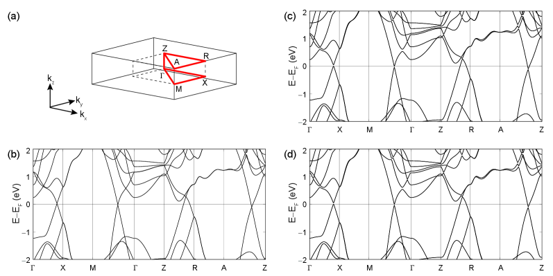
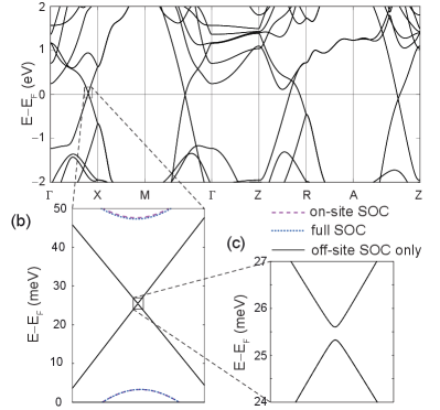
The electronic dispersion of ZrSiS with and without SOC corrections and a standard (DZP) basis set is depicted in Fig. 4. The first Brillouin zone is displayed in Fig. 4(a), Fig. 4(b) contains an electronic dispersion without SOC, while Fig. 4(c) and Fig. 4(d) are band structures with on-site and full SOC, respectively. Visual comparison of Figs. 4(c) and 4(d) indicates that the predominant contribution of SOC comes from on-site interactions (in particular, the gaps at the segment for the on-site and full SOC are both approximately meV).
Fig. 4 shows that contributions beyond the on-site interaction are small already, but we shall be more rigorous and obtain a band structure associated to a system only perturbed by the off-site SOC next. Even though SIESTA does not explicitly provide this option, it stores Hamiltonian and overlap matrices which can thus be examined and manipulated at will. We obtain the off-site SOC dispersion by defining its associated Hamiltonian and overlap matrices as:
| (10) |
where (), (), () and () are the Hamiltonian (overlap) matrices without SOC, with on-site SOC, under off-site, and under full SOC, respectively.
Fig. 5(a) depicts the band structure when only the off-site SOC is turned on. Fig. 5(b) is a zoom-in around the vicinity of the crossing along the segment, where the bands with on-site and full SOC have been included for comparison. The energy gap with just off-site SOC is meV, a value two orders of magnitude smaller than the gap of roughly 20 meV reported in Refs. [4, 46] and the one seen in Fig. 4. Consequently, the gap is due to the on-site SOC predominantly.
The fact that the band gaps around in ZrSiS NLS are predominantly due to an on-site SOC invites to extend the basis of the model beyond Si and orbitals, which will permit observing SOC-gaps without lowering the symmetry of the Si square net [21, 25], and without the need to postulate a SOC interaction that breaks sublattice symmetry ad-hoc [26]. We will develop a TB Hamiltonian with less than 82 orbitals (but more than the four ones used in the models) in Sec. IV. That TB model will reproduce SOC-induced energy gaps due to an on-site SOC. We will embed this SOC into the model through Löwdin partitioning method subsequently (Sec. V).
IV DFT-based TB models with basis sets smaller than DZP to isolate effective on-site SOC effects
IV.1 Rationale
We now design a DFT-based TB description for ZrSiS to identify the orbitals involved in the SOC-induced band gap openings. As indicated in Sec. III, the on-site SOC will suffice, and it will be utilized from now on.
One route toward TB models from DFT involves post-processing of a Hamiltonian originally written on a plane-wave basis set, into a basis of maximally localized Wannier functions [47, 48]. We follow another (similar) approach here: starting with the DFT-Hamiltonian written in a localized basis consisting of atomic orbitals [31, 32], we reduce the number of orbitals and their radial extent gradually. This will shed light into SOC-induced sublattice symmetry breaking on NLSs in this material family, which is the point of this manuscript.
IV.2 Reducing the size of the orbital basis set
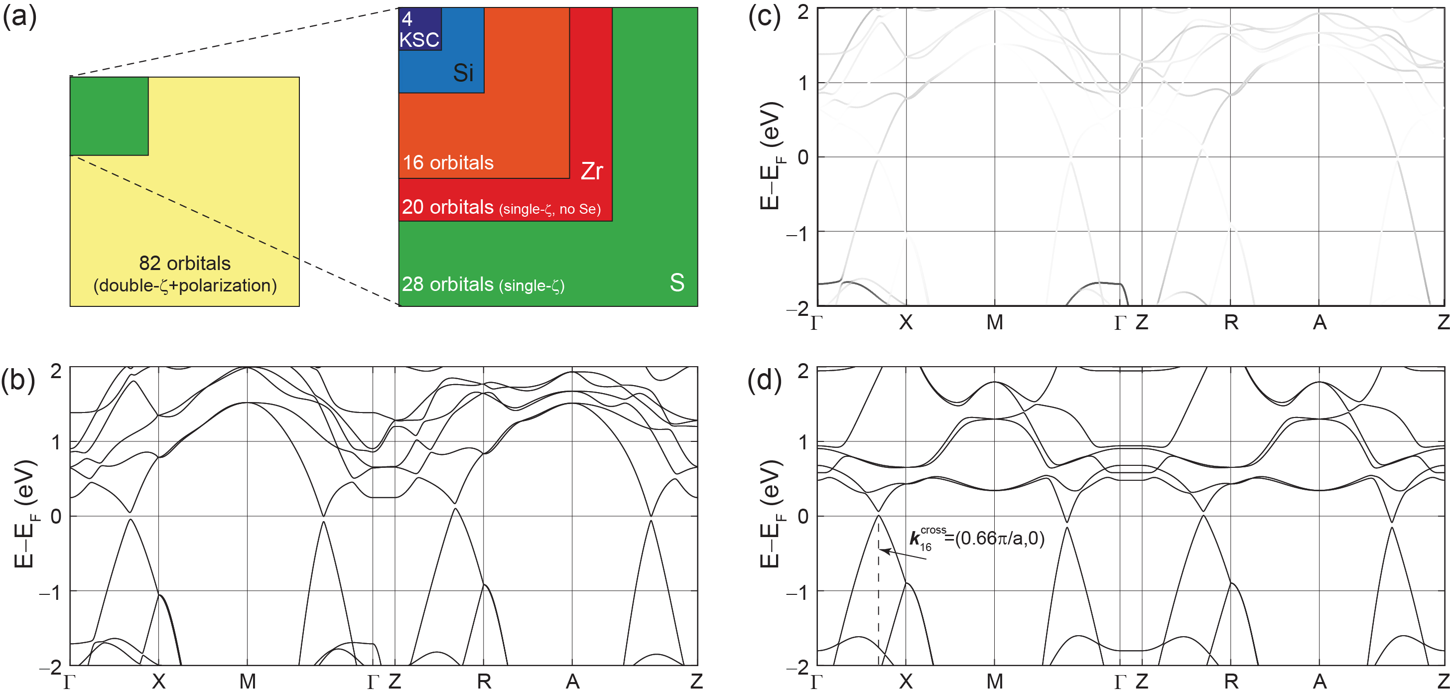
As displayed in Table 2, our initial band structure calculation for ZrSiS relied on 82 atomic orbitals, and the Hamiltonian doubled in size when SOC was included. We wish to determine orbitals with leading contributions to the on-site SOC and–as seen in Table 2–our search included a single (SZ) basis set for Zr, Si, and S (which contains one radial function per valence channel, and no polarizing orbitals) with 28 orbitals, a SZ set for Zr and Si only (which effectively removed S from the electronic structure) with 20 orbitals, and a smaller orbital set with 16 orbitals, in which the and orbitals of Zr were removed. The basis set of models containing four orbitals is shown in Table 2 as well. Fig. 6(a) represents the gradual size reduction of the (square) Hamiltonian matrices achieved as the basis sets were reduced in size.
The band structure shown in Fig. 6(b) was created with the (28-orbital) SZ basis set. The radial cutoffs of the numerical atomic orbitals [32] were set to 2.12 Å to admit second nearest-neighbor interactions at most. The overlap matrix was approximated as the identity matrix in order to reduce the number of parameters on the TB representation. The on-site SOC was included on this Hamiltonian [41], leading to the gapped electronic dispersion around . The crucial observation is that the inclusion of additional orbitals to the Hamiltonian set leads onto gap openings by on-site SOC only.
| Basis set name | Zr | Si | Se | Size of Hamiltonian |
|---|---|---|---|---|
| DZP | 15 | 13 | 13 | 82 |
| SZ | 6 | 4 | 4 | 28 |
| 20-orbital set | 6 | 4 | 0 | 20 |
| 16-orbital set | 4 | 4 | 0 | 16 |
| 0 | 2 | 0 | 4 |
The TB Hamiltonian can be further simplified, while still preserving its crucial qualitative features. The SZ basis set for ZrSiS contains 14 orbitals (Si , , , ; Zr , , , , , ; S , , , ), yielding 28 orbitals per u.c. To discard orbitals, we computed their contribution to the energy bands around . This was done by determining the eigenvectors for every band at each -point. Fig. 6(c) displays the projection of S orbitals onto the electronic dispersion of the 28 orbital model with on-site SOC. The darker the hue, the stronger the contribution. S orbitals barely contribute to the states within Fig. 6(c) and hence can be removed from the basis set without a significant distortion of the low energy electronic dispersion. Analogously, further removal of the and orbitals of Zr still leads to a gapped band structure around when the on-site SOC is turned on; Fig. 6(d) depicts the band structure of the resulting (16-orbital) TB electronic dispersion. The avoided band crossing takes place at .
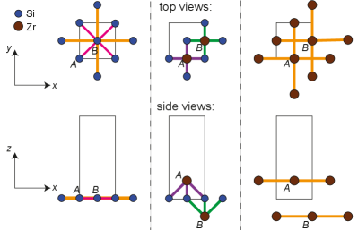
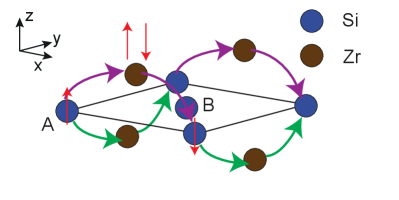
This 16-orbital model provides a qualitative understanding of the origin of SOC in ZrSiS: Fig. 7 illustrates our labelling convention. One Si atom is located at the origin of coordinates, at the corner of the prism in Fig. 1. The Si atom lies at the center of the base. Each Si layer is “sandwiched” by two layers of Zr symmetrically separated. The top Zr layer (above the Si layer) is made of atoms, while Zr atoms conform the bottom layer (below the Si layer). Colored lines in Fig. 7 link the atoms whose interaction is taken into account for this model (Appendix A). Orange and pink lines link atoms located at the same layer, purple links Zr’s atom with the Si layer below it, while green links Zr’s atom with the Si layer above it. As we can observe, the same chemical species only interact with each other when they are located at the same layer: Zr’s and atoms do not interact with each other. Interlayer hopping only happens between Zr atoms and the closest layer of Si atoms.
Furthermore, for a given pair of Si atoms separated by an in-plane lattice constant (i.e. belonging to the same sublattice), there is an associated Zr atom whose in-plane projection lies halfway between the two Si. When the Si atoms belong to the A sublattice, and their relative separation is along the x-direction (), their associated Zr is above the Si layer. In contrast, if such pair of Si atoms belongs to the B sublattice, the associated Zr would be below. It is this difference what produces the sublattice asymmetry discussed in Sec. II for the case of ZrSiS.
IV.3 Spin components
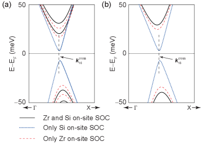
At this point, we have identified the main atomic orbitals involved in the gap opening process, however, we can still be more specific and determine the atom whose on-site SOC contributes the most. Fig. 8(a) displays a zoom-in around the band gap generated by on-site SOC (black bands). The red and blue bands are obtained when only Zr or Si on-site SOC contributions are considered, respectively. Since Si on-site SOC gap is times smaller than the gap seen in Fig. 4(d), we can neglect its contribution to simplify the model. This is an important difference among the model that we are developing and the models discussed in Sec. II: The SOC produced by the atoms in the square net is not required to gap the Fermi level. Rather, the on-site Zr SOC suffices.
Furthermore, on-site SOC couples orbitals with the same spin (i.e. through matrix elements of the form ) or with opposite spins () [41]. Fig 8(b) is a zoom-in at the on-site gap generated by recourse to only matrix elements that couple orbitals with opposite spins. Analogously to Fig 8(a), in Fig 8(b) red, blue, and black bands arise from Zr on-site SOC, Si on-site SOC, and both (Zr and Si) on-site SOC, respectively. The coupling among opposite spins is responsible for the band splitting at .
The SOC due to the four Zr orbitals in the 16-band model looks as follows:
| (11) |
The matrix entries in Eqn. (11) were ordered as follows: , , , , , , , and . The important point is that, unlike and orbitals in Eqn. (4), on-site SOC in Zr does mix spin components. As shown in Fig. 8, such coupling of opposite spins is behind the band gap opening seen in DFT calculations.
The 16-orbital Hamiltonian (Si: , , , ; Zr: , , , ) strikes a balance among basis size and a proper qualitative description of the electronic dispersion with on-site SOC. The parameters for this TB Hamiltonian are provided in Appendix A, and our code is provided in the Supplemental Material. We will consider only Zr on-site SOC among orbitals with opposite spins in next section.
V Adding SOC into the model from a Lödwin partitioning of the 16-orbital Hamiltonian
Löwdin partitioning will now be used [49, 50] to project the on-site SOC due to Zr within the 16-orbital model onto the (4-orbital) Si Hamiltonian at the vicinities of their crossing points ( and , respectively). The first steps are a diagonalization without SOC of both the 16-orbital Hamiltonian () and the one (), and a rearrangement of the diagonalized Hamiltonians, such that the two double degenerate bands around (that we call “low-energy” bands) appear at the four uppermost entries:
| (12) |
(the curly emphasizes that those Hamiltonians without SOC are all diagonal, and is a small excursion away from the points where the crossing takes place). The point is for the “low-energy blocks”, and , to describe the same two double degenerate bands despite them belonging to different models:
| (13) |
up to a scaling factor.
To be specific, let and be the unitary matrices that diagonalize the unperturbed and 16-orbital Hamiltonians, respectively, such that the eigenvalues are ordered at , with eigenvectors and (plus and minus signs label the two orthogonal spin components) (Fig. 9(a)) taking the uppermost four entries:
| (14) |
To add SOC to we must express it in the same basis:
| (15) |
where the superscript in emphasizes that it is only Zr on-site SOC what is being taken into account. As the low-energy bands are gapped under Zr on-site SOC in the 16-orbital model, its low-energy block will be perturbed, however, in general will not be block diagonal, which implies that will not be block diagonal either.
Löwdin partitioning method transforms arbitrary perturbations into a block-diagonal form, nevertheless, so that the vector spaces associated to the low and high energy bands are uncoupled again. Furthermore, the zeroth-order Löwdin partition scheme is to neglect non-block-diagonal terms, giving rise to the gapped electronic dispersion of the low-energy block shown in Fig. 9(b), which is a promising step towards a 4-orbital model with SOC. Our numerical results lead to a SOC perturbation of the low-energy matrix block of the 16-orbital Hamiltonian with SOC [41]:
| (16) |
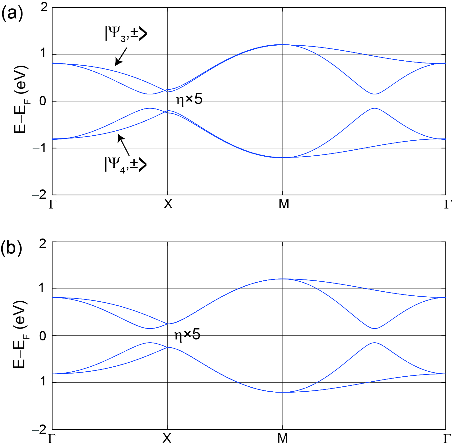
at the vicinity of the band crossing, and in the basis of eigenvectors , which are explicitly provided in Table 3. Here, is a complex parameter that depends on ; meV. We add this perturbation onto the low-energy block of the model in Fig. 9(c), thus finally embedding it with a DFT-based, effective SOC coupling.
| Orbital | ||||
|---|---|---|---|---|
| 0.000 | 0.021-0.284i | - | - | |
| 0.000 | -0.561-0.041i | - | - | |
| -0.063i | 0.000 | - | - | |
| 0.569 | 0.000 | - | - | |
| 0.000 | 0.021-0.284i | - | - | |
| 0.000 | 0.561+0.041i | - | - | |
| -0.063i | 0.000 | - | - | |
| -0.569 | 0.000 | - | - | |
| -0.182 | 0.000 | - | - | |
| 0.337i | 0.000 | -0.787+0.618i | 0.000 | |
| 0.000 | 0.318+0.023i | 0.000 | 0.787-0.618i | |
| -0.160 | 0.000 | - | - | |
| 0.182 | 0.000 | - | - | |
| -0.337i | 0.000 | 0.787+0.618i | 0.000 | |
| 0.000 | 0.318+0.023i | 0.000 | 0.787+0.618i | |
| -0.160 | 0.000 | - | - |
Now, given that the SOC perturbation only affected the bands that produced the crossing, the remaining two bands in the dispersion are still unmodified. In Fig. 10(a), we show the bands of the model once has been added to its low-energy block. Löwdin procedure only addresses how the dispersion around is modified, however, a characteristic of ZrSiS is the symmetry-protected crossing at , which is not observed in Fig. 10(a). To recover such degeneracy, the two high-energy bands in the model (Fig. 3) must also be modified. Analogously to the low-energy block, we add an high-energy SOC Hamiltonian:
| (17) |
which is now written in the basis , , , . Thus, the effective on-site SOC inherited from Zr in the model can be expressed as:
| (18) |
and the Hamiltonian under the effective on-site SOC expressed in the eigenbasis of the unperturbed Hamiltonian happens to be:
| (19) |
with an associated dispersion degenerate at depicted in Fig 10(b) (see a similar degeneracy in Figs. 4(c), 4(d), 6(b), and 6(d)).
The last question is whether SOC makes the Si and sublattices inequivalent. To answer this, we transformed the SOC Hamiltonian back into the original basis (, ), to get:
| (20) |
where has the form:
| (21) |
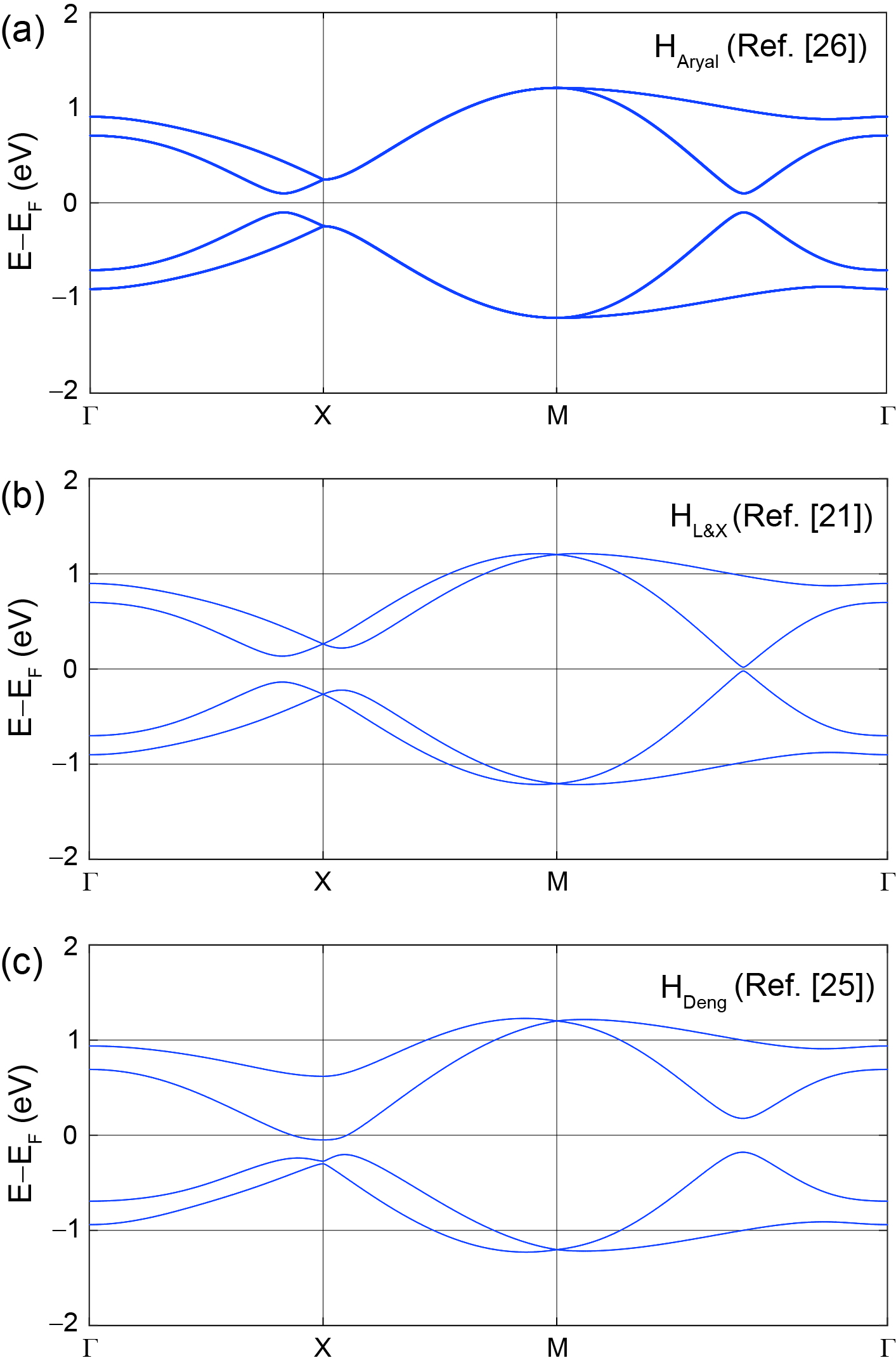
along the segment: Zr’s on-site SOC did produce an inequivalence among A and B sublattices on the model, as the hopping from to has opposite sign with respect to the hopping from to at the crossing at . Thus, Zr is responsible for the lowering of symmetry that Refs. [21] and [25] assigned to the atoms within their square nets, and which Ref. [26] postulated ad hoc. Fig. 11 displays the band structures of the models with SOC plus the sublattice asymmetric perturbations discussed in Sec. II for comparison with our model.
The correct, actual SOC Hamiltonian for ZrSiS–obtained with DFT guidance here–can also be expressed in terms of the Pauli matrices introduced in Sec. II, and it is our main contribution:
| (22) |
The picture that arises as a result is as follows: Fig 12 displays the trajectories that an electron originally with spin up follows to connect with atoms on the same sublattice. The electron will first hop to a Zr atom, which will be in charge of switching its spin through on-site SOC. Then, it will hope again to a Si atom of the same sublattice to produce an effective hopping term that acquires the value of in the vicinity of . Observe that, depending on the direction of hopping (horizontal versus vertical), the electron will pass either under or over the Si layer. Since the relative positions of neighboring Zr atoms depends on the sublattice, the presence of Zr facilitates the asymmetry observed in Eq. (21).
Informed by DFT, we have systematically showed how to embed Zr on-site SOC into the model for ZrSiS. In this manner, we not only connect the observations made in previous works, but also, we show that on-site SOC does not require the addition of extra terms to gap the dispersion around the Fermi level.
VI Conclusions
In this work, we followed a systematic procedure to induce a gap in the model. Relying on DFT all along, we concluded that (i) on-site SOC is the main responsible to the SOC-gaps reported on the band structure of ZrSiS around . Furthermore, (ii) we determined that Zr’s orbitals play a key role on the on-site SOC, and that coupling among opposite spins is crucial to split degenerate bands around . Then, (iii) we developed a DFT-based TB model larger than , but smaller than the DZP one, which allowed to treat SOC carefully. At that point, (iv) we applied a Lödwin decomposition to extract an effective SOC, and ended up with a dispersion gapped at and consistent with DFT, without arbitrary lowering the symmetry of the square net, nor postulating the entries of the SOC interaction in an ad hoc manner. This model extends the usefulness of the minimal square-net nodal line semimetal TB models.
Acknowledgements.
G.S.O.G. and S.B.L. acknowledge partial funding from the MonArk NSF Quantum Foundry, supported by the National Science Foundation Q-AMASE-i program under NSF award No. DMR-1906383. Calculations were performed at the University of Arkansas’ Pinnacle supercomputer, funded by the U.S. National Science Foundation, the Arkansas Economic Development Commission, and the Office of the Vice Provost for Research and Innovation. A.G.F. was funded by project PID2022-137078NB-I00 (MCIU/AEI/FEDER, EU) and Asturias FICYT under Grant No. AYUD/2021/51185 with the support of FEDER funds. We thank A. Huamán for his assistance with the Lödwin projection scheme. Conversations with A. Fereidouni Ghaleh Minab, J. Hu, and J. Ferrer are gratefully acknowledged.References
- Gao et al. [2019] H. Gao, J. W. Venderbos, Y. Kim, and A. M. Rappe, Annu. Rev. Mater. Res. 49, 153 (2019).
- Young and Kane [2015] S. M. Young and C. L. Kane, Phys. Rev. Lett. 115, 126803 (2015).
- Kruthoff et al. [2017] J. Kruthoff, J. De Boer, J. Van Wezel, C. L. Kane, and R.-J. Slager, Phys. Rev. X 7, 041069 (2017).
- Schoop et al. [2016] L. M. Schoop, M. N. Ali, C. Straßer, A. Topp, A. Varykhalov, D. Marchenko, V. Duppel, S. S. Parkin, B. V. Lotsch, and C. R. Ast, Nat. Commun. 7, 1 (2016).
- Hu et al. [2016] J. Hu, Z. Tang, J. Liu, X. Liu, Y. Zhu, D. Graf, K. Myhro, S. Tran, C. N. Lau, J. Wei, and Z. Mao, Phys. Rev. Lett. 117, 016602 (2016).
- Singha et al. [2017] R. Singha, A. K. Pariari, B. Satpati, and P. Mandal, PNAS 114, 2468 (2017).
- Sankar et al. [2017] R. Sankar, G. Peramaiyan, I. P. Muthuselvam, C. J. Butler, K. Dimitri, M. Neupane, G. N. Rao, M.-T. Lin, and F. Chou, Sci. Rep. 7, 40603 (2017).
- Ali et al. [2016] M. N. Ali, L. M. Schoop, C. Garg, J. M. Lippmann, E. Lara, B. Lotsch, and S. S. Parkin, Sci. Adv. 2, e1601742 (2016).
- Voerman et al. [2019] J. Voerman, L. Mulder, J. De Boer, Y. Huang, L. Schoop, C. Li, and A. Brinkman, Phys. Rev. Mater. 3, 084203 (2019).
- Wang et al. [2016] X. Wang, X. Pan, M. Gao, J. Yu, J. Jiang, J. Zhang, H. Zuo, M. Zhang, Z. Wei, W. Niu, et al., Adv. Electron. Mater. 2, 1600228 (2016).
- Zhang et al. [2018] J. Zhang, M. Gao, J. Zhang, X. Wang, X. Zhang, M. Zhang, W. Niu, R. Zhang, and Y. Xu, Front. Phys. 13, 1 (2018).
- Schilling et al. [2017] M. Schilling, L. Schoop, B. Lotsch, M. Dressel, and A. Pronin, Phys. Rev. Lett. 119, 187401 (2017).
- fu2 [2019] Sci. Adv. 5, eaau6459 (2019).
- Teicher et al. [2022] S. M. Teicher, J. F. Linnartz, R. Singha, D. Pizzirani, S. Klemenz, S. Wiedmann, J. Cano, and L. M. Schoop, Chem. Mater 34, 4446 (2022).
- Banerjee and Saxena [2021] S. Banerjee and A. Saxena, Phys. Rev. B 103, 235125 (2021).
- Michen and Budich [2022] B. Michen and J. C. Budich, Phys. Rev. Res. 4, 023248 (2022).
- Rosmus et al. [2022] M. Rosmus, N. Olszowska, Z. Bukowski, P. Starowicz, P. Piekarz, and A. Ptok, Mater. 15, 7168 (2022).
- He [2021] C. He, EPL 133, 27003 (2021).
- Herrera and Bercioux [2023] M. A. Herrera and D. Bercioux, Commun. Phys. 6, 42 (2023).
- Cano et al. [2021] J. Cano, S. Fang, J. Pixley, and J. H. Wilson, Phys. Rev. B 103, 155157 (2021).
- Luo and Xiang [2015] W. Luo and H. Xiang, Nano Lett. 15, 3230 (2015).
- Klemenz et al. [2019] S. Klemenz, S. Lei, and L. M. Schoop, Annu. Rev. Mater. Res. 49, 185 (2019).
- Klemenz et al. [2020a] S. Klemenz, A. K. Hay, S. M. Teicher, A. Topp, J. Cano, and L. M. Schoop, J. Am. Chem. Soc. 142, 6350 (2020a).
- Klemenz et al. [2020b] S. Klemenz, L. Schoop, and J. Cano, Phys. Rev. B 101, 165121 (2020b).
- Deng et al. [2022] J. Deng, D. Shao, J. Gao, C. Yue, H. Weng, Z. Fang, and Z. Wang, Phys. Rev. B 105, 224103 (2022).
- Aryal et al. [2022] N. Aryal, Q. Li, A. Tsvelik, and W. Yin, Phys. Rev. B 106, 235116 (2022).
- Yang et al. [2021] Y. Yang, H. Xing, G. Tang, C. Hua, C. Yao, X. Yan, Y. Lu, J. Hu, Z. Mao, and Y. Liu, Phys. Rev. B 103, 125160 (2021).
- Konschuh et al. [2010] S. Konschuh, M. Gmitra, and J. Fabian, Phys. Rev. B 82, 245412 (2010).
- Barraza-Lopez and Naumis [2022a] S. Barraza-Lopez and G. G. Naumis, J. Phys.: Condens. Matter 35, 035502 (2022a).
- Martin [2020] R. M. Martin, Electronic Structure: Basic Theory and Practical Methods, 2nd ed. (Cambridge University Press, 2020).
- Soler et al. [2002] J. M. Soler, E. Artacho, J. D. Gale, A. García, J. Junquera, P. Ordejón, and D. Sánchez-Portal, J. Phys.: Condens. Matter 14, 2745 (2002).
- Junquera et al. [2001] J. Junquera, O. Paz, D. Sánchez-Portal, and E. Artacho, Phys. Rev. B 64, 235111 (2001).
- Barraza-Lopez et al. [2010] S. Barraza-Lopez, M. Vanević, M. Kindermann, and M. Y. Chou, Phys. Rev. Lett. 104, 076807 (2010).
- Mehboudi et al. [2016] M. Mehboudi, B. M. Fregoso, Y. Yang, W. Zhu, A. van der Zande, J. Ferrer, L. Bellaiche, P. Kumar, and S. Barraza-Lopez, Phys. Rev. Lett. 117, 246802 (2016).
- Barraza-Lopez et al. [2009] S. Barraza-Lopez, K. Park, V. García-Suárez, and J. Ferrer, Phys. Rev. Lett. 102, 246801 (2009).
- Fernández-Seivane et al. [2006] L. Fernández-Seivane, M. A. Oliveira, S. Sanvito, and J. Ferrer, J. Phys.: Condens. Matter 18, 7999 (2006).
- Cuadrado et al. [2021] R. Cuadrado, R. Robles, A. García, M. Pruneda, P. Ordejón, J. Ferrer, and J. I. Cerdá, Phys. Rev. B 104, 195104 (2021).
- Martinez-Carracedo et al. [2023] G. Martinez-Carracedo, L. Oroszlány, A. García-Fuente, B. Nyári, L. Udvardi, L. Szunyogh, and J. Ferrer (2023), arXiv:2309.02558.
- Sloan et al. [2013] J. V. Sloan, A. A. P. Sanjuan, Z. Wang, C. Horvath, and S. Barraza-Lopez, Phys. Rev. B 87, 155436 (2013).
- Naumis et al. [2017] G. G. Naumis, S. Barraza-Lopez, M. Oliva-Leyva, and H. Terrones, Rep. Prog. Phys. 80, 096501 (2017).
- Barraza-Lopez and Naumis [2022b] S. Barraza-Lopez and G. G. Naumis, J. Phys.: Condens. Matter 35, 035502 (2022b).
- Slater and Koster [1954] J. C. Slater and G. F. Koster, Phys. Rev. 94, 1498 (1954).
- Note [1] Supplemental Material contains a description of the on-site SOC, a MATLAB program to reproduce the bands of the 16-orbital model and to obtain the parameter from Löwdin partitioning technique, and a TB electronic dispersion of slabs using the 16-orbital model.
- Kurita and Koretsune [2020] K. Kurita and T. Koretsune, Phys. Rev. B 102, 045109 (2020).
- Cuadrado and Cerdá [2012] R. Cuadrado and J. Cerdá, J. Condens. Matter Phys. 24, 086005 (2012).
- Hosen et al. [2017] M. M. Hosen, K. Dimitri, I. Belopolski, P. Maldonado, R. Sankar, N. Dhakal, G. Dhakal, T. Cole, P. M. Oppeneer, D. Kaczorowski, et al., Phys. Rev. B 95, 161101 (2017).
- Wannier [1937] G. H. Wannier, Phys. Rev. 52, 191 (1937).
- Marzari et al. [2012] N. Marzari, A. A. Mostofi, J. R. Yates, I. Souza, and D. Vanderbilt, Rev. Mod. Phys. 84, 1419 (2012).
- Löwdin [1963] P.-O. Löwdin, J of Mol. Spectrosc. 10, 12 (1963).
- Roland [2003] W. Roland, Springer Tracts in Modern Physics 191 (2003).
Appendix A Tight binding description from DFT
To construct a TB model, it is necessary to compute two-center integrals of the form [42]:
| (23) | ||||
| (24) |
where and are atomic positions in which localized orbitals and are centered at, respectively.
SIESTA [31] constructs an auxiliary supercell, and then proceeds to calculate the two center integrals between each orbital within the u.c. with every orbital in the supercell. The information of these integrals, written into text files, is used to explicitly build the entries of the Hamiltonian for each point in reciprocal space here:
| (25) |
where the primed index runs over the full supercell and implies that is the unit cell counterpart of .
For elements containing up to electrons, Slater and Koster proposed that the values of these two center integrals can be expressed as [42, 30]:
| (26) |
where are the known TB parameters while are functions of the projection cosines , and that can be explicitly found in the original work of Slater and Koster [42].
Once positions of the atoms and the values of the two-center integrals are known, the TB parameters associated to the orbitals and can be obtained by solving the system of linear equations of the form of Eqn. (26), generated by and the set of orbitals in the supercell whose equivalent orbital in the u.c. is . Typically, these systems will be overdetermined–there are more neighbors than unknown parameters. There can be instances where and still . Even though the contribution of such integrals cannot be considered in the Slater-Koster approximation, excluding them does not brake any symmetries and we have found that the change in the dispersion of the bands is negligible.
In the following subsection, we report a TB description of the 16-orbital Hamiltonian. The parameters used to build the model were obtained by solving systems of linear equations as described in the present subsection.
A.1 16-orbital model
To produce the dispersion depicted in Fig. 6(d), we label the atoms in the u.c. first. In this model, S orbitals have already been excluded from the basis set. Fig. 7 illustrates our labelling convention. We define the Hamiltonian matrix that takes into account interactions in sub-blocks of matrices:
| (27) |
Each block contains the information of the interaction of all the orbitals of one atom with every orbital of another atom. The order of the block rows and columns is ZrB, ZrA, SiA, SiB (i.e. contains the information of the interaction among ZrA and SiA orbitals).
Using the Slater-Koster approach, we wrote the entries of each block in terms of the lattice vectors (Table 4), the displacement vectors (Table 5), and the TB parameters (Table 6). Recalling that the projection cosines , , , along , , respectively are defined by:
the non-zero matrix elements of the Hamiltonian expressed in the basis: Si: , , , ; Zr: , , , , are written in Table7.
| Lattice constants |
|---|
| , |
| Lattice vectors |
| , , |
| SiA-SiB |
| , , |
| , |
| ZrA-SiA |
| , , |
| ZrA-SiB |
| , , |
| ZrB-SiA |
| , , |
| ZrB-SiB |
| , , |
| Zr-Zr and Si-Si |
| , , , |
. Atom () Orbital () 1 Zr 0.0000 3.199 2 3.220 3 3.239 4 Si 0.0000 -5.179 5 2.301 6 2.564 AtomR AtomC () OrbR OrbC () 1 Si Si 2.5062 -1.690 2 -2.207 3 2.207 4 1.691 5 3.046 6 -0.680 7 Zr Si 2.8210 0.522 8 1.141 9 1.425 10 -1.685 11 -0.535 12 -1.128 13 -0.634 14 2.168 15 Si Si 3.5440 -0.139 16 -0.279 17 0.555 18 Zr Zr 3.6460 -0.407
| SiA-SiB () |
|---|
| , |
| , |
| , |
| , |
| , |
| , |
| , |
| , |
| ZrA-SiA (;), ZrB-SiB (;) |
| , |
| , |
| , |
| , |
| , |
| , |
| , |
| ZrA-SiB (;), ZrB-SiA (;) |
| , |
| , |
| , |
| , |
| , |
| , |
| , |
| , |
| Zr-Zr and Si-Si () |
| , |
| , |
| , |
| , |
| , |
| , |
| , |
| , |