Tightness of exponential metrics for log-correlated Gaussian fields in arbitrary dimension
Abstract
We prove the tightness of a natural approximation scheme for an analog of the Liouville quantum gravity metric on for arbitrary . More precisely, let be a suitable sequence of Gaussian random functions which approximates a log-correlated Gaussian field on . Consider the family of random metrics on obtained by weighting the lengths of paths by , where is a parameter. We prove that if belongs to the subcritical phase (which is defined by the condition that the distance exponent is greater than ), then after appropriate re-scaling, these metrics are tight and that every subsequential limit is a metric on which induces the Euclidean topology. We include a substantial list of open problems.
Acknowledgments. We thank Karim Adiprasito, Timothy Budd, Hugo Falconet, Josh Pfeffer, Scott Sheffield, and Xin Sun for helpful discussions. J.D. is partially supported by NSFC Key Program Project No. 12231002. E.G. was partially supported by a Clay research fellowship and by NSF grant DMS-2245832. Z.Z. was partially supported by NSF grant DMS-1953848.
1 Introduction
There has been an enormous amount of research in the past several decades concerning random geometry in two dimensions. Some of the major topics in this subject include Schramm-Loewner evolution, conformal field theory, statistical mechanics models on planar lattices, random planar maps, Liouville quantum gravity, and random geometries related to the KPZ universality class. We will not attempt to survey this vast literature here, but see, e.g., [sheffield-icm, gwynne-ams-survey, bp-lqg-notes, bn-sle-notes, pw-gff-notes, ghs-mating-survey, vargas-dozz-notes, legall-sphere-survey, ganguly-dl-survey] for some recent expository articles. However, most of the results in this area have not been extended to higher dimensions. One reason for this is that conformal invariance (or covariance) plays a central role in many of the results in two dimensions, and there are no non-trivial conformal maps in higher dimensions. Another reason is that many of the arguments in the two-dimensional case rely on topological properties which are not true in higher dimensions, e.g., the Jordan curve theorem.
In this paper, we consider the problem of constructing an analog of the Liouville quantum gravity (LQG) metric on , for arbitrary . Heuristically speaking, LQG is the random geometry described by the random Riemannian metric tensor
| (1.1) |
where is a parameter, is the Euclidean metric tensor, and is a variant of the Gaussian free field (GFF) on (or more generally on a Riemann surface). See, e.g., [shef-gff, bp-lqg-notes, pw-gff-notes] for an introduction to the GFF. The definition (1.1) does not make literal sense since is a generalized function (distribution) instead of a true function, so its exponential cannot be defined pointwise. Nevertheless, one can define various objects associated with (1.1) by replacing with a sequence of continuous functions which approximate , then taking an appropriate limit.
Perhaps the easiest object to construct in this way is the LQG area measure, which is a limit of regularized versions of (where denotes Lebesgue measure). The construction of this measure is a special case of the theory of Gaussian multiplicative chaos (GMC), which allows one to make sense of random measures of the form for , whenever is a log-correlated Gaussian field on a domain (for arbitrary ) and is an appropriate deterministic base measure on . See [shef-kpz, rhodes-vargas-review, bp-lqg-notes] for more on Gaussian multiplicative chaos and the LQG area measure.
Recent works have also constructed the Riemannian distance function associated with (1.1), i.e., the LQG metric. This is a random metric on constructed as follows. For , let be the convolution of the Gaussian free field with the heat kernel . Also let , where is the so-called LQG dimension exponent [dg-lqg-dim]. Then, let
| (1.2) |
where the infimum is over all piecewise continuously differentiable paths from to . The papers [dddf-lfpp, gm-uniqueness] prove that there exist normalizing constants such that converges in probability to a limiting metric with respect to the topology of uniform convergence on compact subsets of (the convergence in probability was recently improved to a.s. convergence in [devlin-lfpp-as]). In particular, it was shown in [dddf-lfpp] that the approximating metrics are tight, and in [gm-uniqueness] (building on [local-metrics, gm-confluence, lqg-metric-estimates]) that the subsequential limit is unique. The proofs in these papers are much more difficult than the proofs in the construction of the LQG area measure. Intuitively, this is because the minimizing path in (1.2) depends on . See [ddg-metric-survey] for a survey of known results about the LQG metric.
In light of the theory of Gaussian multiplicative chaos, it is natural to wonder whether there is an analogous theory of exponential metrics associated with log-correlated Gaussian fields on for arbitrary111Note that when , the metric induced by is simply given by the one-dimensional GMC measure, as any path in is an interval. , which generalizes the LQG metric. The construction of such a theory is listed as Problem 7.19 in [gm-uniqueness].
This paper carries out the first major step toward such a theory: namely, we prove the tightness of a natural approximation scheme similar to (1.2) for log-correlated Gaussian fields on (in the full subcritical phase of values). That is, we carry out the higher-dimensional analog of [dddf-lfpp]. See Theorem 1.2 below for a precise statement. We expect that it will be challenging, but possible to prove that the subsequential limit is unique (and characterized by a list of axioms similar to the ones which characterize the LQG metric in dimension two [gm-uniqueness]) by adapting the arguments in the two-dimensional case [gm-uniqueness, dg-uniqueness]. Indeed, these arguments do not use two-dimensionality in as fundamental a way as the proof of tightness in [dddf-lfpp]. See Problem LABEL:prob:uniqueness for further discussion.
More speculatively, our limiting metric might have connections to other higher-dimensional extensions of objects related to LQG, e.g., Liouville conformal field theory in even dimensions [cercle-higher-dimension, dhks-even-dim], the higher-dimensional analogs of the Brownian map considered in [ml-iterated-folding], uniform samples from various classes of triangulations of higher-dimensional spheres (see, e.g., [bz-locally-constructible, dj-3-manifolds]), higher-dimensional analogs of random planar maps constructed from trees [BC23, budd-lionni-3-spheres], and random graphs in arising from sphere packings (see, e.g., [bc-sphere-packing]). See Subsection 1.2 for more details.
The problem of constructing natural random Riemannian metrics in dimension is also of substantial interest in theoretical physics in the context of quantum gravity (see, e.g., the books [gh-quantum-gravity, adj-quantum-geometry, rovelli-quantum-geometry]). We refer to the introductions of [BC23, budd-lionni-3-spheres] for additional relevant discussion and references.
The proofs in this paper are by necessity substantially different than those in the two-dimensional case [dddf-lfpp]. In particular, we do not have an a priori Russo-Seymour-Welsh (RSW) type estimate (which in the two-dimensional case comes from a conformal invariance argument), and various path-joining arguments in [dddf-lfpp] do not work in higher dimensions. For these reasons, we use a fundamentally novel approach to proving tightness which bypasses any direct proofs of RSW estimates as well as the use of the Efron-Stein inequality. See Subsection 1.3 for details.
The results of this paper open up a number of interesting questions about random metrics on . See Section LABEL:sec:open-problem for a discussion of some open problems.
1.1 Definitions and main result
We now introduce some notation and state the main result of this paper. We consider the space with and define the box
| (1.3) |
Fix a smooth function and such that
-
1.
K is radially symmetric, meaning that for any with the same Euclidean norm.
-
2.
K is supported222 We expect that our arguments can be adapted to the case when K is not compactly supported but has sufficiently rapid decay at . This would require some added technicalities similar to ones encountered in [dddf-lfpp]. However, the choice of K in this paper is in some sense unimportant since, regardless of the choice of K, the fields we consider are closely related to the canonical log-correlated Gaussian field on considered in [lgf-survey, fgf-survey] (see Remark 1.4). in the box .
-
3.
K is normalized such that .
We also let be a space-time white noise on . That is, is the Gaussian random generalized function on such that for any , the formal integral is centered Gaussian with variance .
We consider a log-correlated Gaussian field and its approximation , defined as follows:
| (1.4) | ||||
for and integer . From the definition of , we see that and are centered Gaussian processes with covariance kernels
| (1.5) |
where denotes the convolution. Using the representation (1.4) and the fact that is a random tempered distribution (see e.g. Section 2.3 of [fgf-survey]), one can verify that each has a modification which is a smooth function (see also Proposition 2.1 of [df-lqg-metric]). We henceforth assume that each has been replaced by such a modification. Furthermore, from (1.1) we get for each . The process is interpreted as a generalized function, and is closely related to the log-correlated Gaussian field on considered in [lgf-survey, fgf-survey] (see Remark 1.4).
Analogously333As explained in [dddf-lfpp] (see also [cg-support-thm, Section 3.1]), in the two-dimensional case, the convolution of the planar Gaussian free field with the heat kernel (at an appropriate -dependent time) has the same law as the field of (1.4) with , up to adding a random continuous function. Hence (1.6) is directly analogous to (1.2). To avoid unnecessary technical work, in this paper we require that K is compactly supported, but we expect that our results can be fairly easily extended to the case where K is not compactly supported but has sufficiently fast decay at . to (1.2), for a parameter , we define the exponential metric associated with as follows:
| (1.6) |
where the infimum is taken over all piecewise continuously differentiable paths joining . This can be interpreted as an approximation of the random metric formally given by reweighting the Euclidean lengths of paths by . We will be interested in (subsequential) limits of the renormalized metrics , where the normalizing constant 444For technical reasons, we first work with this particular choice of normalizing constant. However, in the end, we can choose any reasonable normalizing constant, such as the median of or . is defined as:
| (1.7) |
where denotes the minimal -length of a path joining and inside the box .
In Section 3, we will prove the following.
Proposition 1.1.
For each , there exists such that
| (1.8) |
Furthermore, is a continuous, non-increasing function and we have
| (1.9) |
The proof of Proposition 1.1 is via a subadditivity argument. Just like in the two-dimensional case, we do not know the value of explicitly (see Problems LABEL:prob:positive-Q and LABEL:prob:special). Analogously to the two-dimensional case (see [dg-supercritical-lfpp, Equation (1.4)]), we define the critical value
| (1.10) |
See Remark 1.3 for some discussion of why this value is critical. We note that if and only if . The lower bound from (1.9) implies that , and the upper bound implies that . The main result of this paper is the tightness of our approximating metrics in the full subcritical phase.
Theorem 1.2.
When , equivalently , the sequence of metrics is tight with respect to the topology of uniform convergence on compact subsets of . Furthermore, each possible subsequential limit (in distribution) is a metric on which induces the Euclidean topology.
Remark 1.3.
When , we expect that the metrics are not tight with respect to the topology of uniform convergence on compact subsets of . So, our result should be optimal modulo the critical case when . Indeed, the maximum of on a fixed bounded open set should grow like as , see e.g. [Mad15]. From this and the continuity properties of (Claim (2) of Lemma 2.3), if is fixed, then when is large with high probability there exists such that for each in the box . For this choice of , the definition of shows that the -distance from to is at least . By (1.8),
If , then for a small enough choice of , this goes to as , which means that cannot be tight with respect to the local uniform topology.
In the two-dimensional case, it was shown in [dg-supercritical-lfpp, dg-uniqueness] that the re-scaled approximating metrics converge with respect to the topology on lower semicontinuous functions for all (including when ). However, when , the limiting metric does not induce the Euclidean topology on . Rather, there are uncountably many “singular points” which lie at infinite distance from every other point. It is plausible that similar statements are true for general , but we do not address this in the present paper. See Problem LABEL:prob:supercritical.
Remark 1.4.
The field of (1.4) is closely related to the log-correlated Gaussian field on considered in [lgf-survey, fgf-survey]. Indeed, define the random generalized function in the same manner as in (1.4), but with integrated over instead of over . Then, a short computation shows that for any choice of the kernel K above, one can make sense of as a random generalized function viewed modulo additive constant555That is, makes sense whenever is smooth and compactly supported with . and that agrees in law, modulo additive constant, with the log-correlated Gaussian field from [lgf-survey, fgf-survey]. Furthermore, has a modification which is a continuous function, viewed modulo additive constant. This was discussed in [lgf-survey, Section 4.1.1] and explained in detail in the two-dimensional case in [afs-metric-ball, Appendix B] (the same proof works for any dimension). Due to the continuity of , one can easily deduce from Theorem 1.2 that a natural approximation scheme for the exponential metric associated with is also tight.
1.2 Related models
Since the construction of the LQG metric in [dddf-lfpp, gm-uniqueness], there have been several additional works which prove tightness and/or uniqueness for various random fractal metrics. Examples include the supercritical LQG metric [dg-supercritical-lfpp, dg-uniqueness] (as mentioned in Remark 1.3), the conformal loop ensemble chemical distance [miller-cle-metric], and the limit of long-range percolation on [baumler-long-range-perc, dfh-long-range-perc]. We also mention the directed landscape, a random directed metric on related to the KPZ universality class [dov-dl].
An important feature of LQG is its relation with two-dimensional Liouville conformal field theory (LCFT) rigorously constructed in [dkrv-lqg-sphere] and follow-up works. The framework of LCFT can produce exact solvability results for the area and length measures associated with LQG surfaces when the underlying field is well chosen. Recently, two-dimensional LCFT has been extended to even dimensions in the papers [cercle-higher-dimension, dhks-even-dim]. Both of these works construct a log-correlated Gaussian field on a -dimensional manifold whose law is re-weighted according to the so-called Liouville action. In other words, these works carry out analogs of [dkrv-lqg-sphere] on certain -manifolds. It should be possible to use the results of the present paper to associate a random metric with the fields considered in [cercle-higher-dimension, dhks-even-dim], at least as a subsequential limit. As in the two-dimensional case, the exponent of Proposition 1.1 should correspond to the background charge in [cercle-higher-dimension] (which is also called ).
In two dimensions, LQG is conjectured to describe the scaling limit of random planar maps. In particular, the LQG metric is believed to describe the scaling limit of the random planar maps equipped with their graph distance in, e.g., the Gromov-Hausdorff sense. This convergence has been rigorously established for uniform random planar maps toward LQG with (), but is open for other values of . More precisely, it was shown in [legall-uniqueness, miermont-brownian-map] that uniform random planar maps converge to a random metric space called the Brownian map, and in [lqg-tbm1, lqg-tbm2] that the Brownian map is equivalent to -LQG, as a metric space. See also [hs-cardy-embedding] for a stronger topology of convergence and Section 2.4 of [ddg-metric-survey] for further discussions.
It would be extremely interesting to find a natural discrete random geometry in dimension whose scaling limit is described by one of the exponential random metrics considered in this paper (or some minor variant thereof).
In analogy with the case of uniform triangulations in two-dimensions (which converge to -LQG), a natural discrete model to consider is uniform triangulations of the -dimensional sphere, with total -simplices. Such triangulations appear to be very difficult to analyze. For example, it is a well-known open problem to determine whether the number of triangulations of the three-sphere with total tetrahedra grows exponentially or superexponentially [dj-3-manifolds, gromov-spaces]. Moreover, simulations suggest that uniform triangulations of the three-sphere may not have interesting scaling limits when viewed as metric spaces, see, e.g., [bk-3d-simplicial, av-3d-simplicial, abkv-3d-vacuum, ckr-3d-entropy, hty-3d-phases, hin-3d-simulation]. We refer to the introductions of [dj-3-manifolds, bz-locally-constructible, budd-lionni-3-spheres] and the references therein for further discussion.
On the other hand, there are natural restricted classes of triangulations of -spheres which appear to be more tractable, and whose cardinality can be shown to grow exponentially in . Examples include locally constructible, constructible, shellable, and vertex-decomposable triangulations [dj-3-manifolds, bz-locally-constructible]. One could ask whether a uniform sample from any of these restricted classes converges in the Gromov-Hausdorff sense to the exponential metric associated with a log-correlated Gaussian field (or a field which locally looks like a log-correlated Gaussian field).
Another interesting class of -dimensional triangulations which one could consider are those which can be represented as the tangency graph of a sphere packing in (or the -sphere). Unlike for , there is not a simple criterion for when a graph can be represented by a sphere packing in for . In fact, for several values of , it is known that the problem of determining whether a given graph admits a sphere packing representation in is NP hard [hk-disks-and-balls]. In dimension two, circle packings and their links to random conformal geometry are fairly well-understood (see, e.g., the survey [nachmias-circle-packing]). In higher dimensions the theory is much less well-developed and likely to be much more difficult. But, a few results can be found, e.g., in [cr-rigidity, bc-sphere-packing, lee-conformal-growth]. One could look for a natural model of random sphere packings in whose scaling limit is described by the exponential of a log-correlated Gaussian field.
In another direction, connections between -LQG and random planar maps for general have been obtained using the framework of mating-of-trees theory [wedges], see the survey [ghs-mating-survey]. The recent work [BC23] presents an analog of mating-of-trees constructions in three dimensions. In a similar vein, the paper [budd-lionni-3-spheres] introduces a model of random triangulations of the three-sphere, decorated by a pair of trees, which is combinatorially tractable and has interesting geometric features. It is natural to wonder if either of these models are related to the exponential metrics for log-correlated fields in dimension three.
Recently, an analog of the Brownian map in dimension was proposed in [ml-iterated-folding]. It is also natural to wonder whether this random metric space has any relation to the exponential metrics of log-correlated Gaussian fields, analogous to the aforementioned relationship between the Brownian map and -LQG.
1.3 Outline
Here, we outline the proof strategy of Theorem 1.2 and describe the content of each subsequent section.
1.3.1 Comparison to the two-dimensional case
First, let us highlight the main differences between the method in this paper and the methods used in the earlier works [ding-dunlap-lqg-fpp, ding-dunlap-lgd, df-lqg-metric, dddf-lfpp, dg-supercritical-lfpp] to establish the tightness of approximations of exponential metrics for log-correlated fields in two-dimensions. All the results in two dimensions rely crucially on RSW estimates, which give up-to-constants comparisons between quantiles of -crossing lengths of rectangles in the “easy direction” and the “hard direction”, see e.g. Section 3 of [dddf-lfpp]. The arguments to prove these estimates are based on either approximate conformal invariance or on forcing paths to cross each other, neither of which works in higher dimensions. For this reason, we will use a fundamentally different approach to prove tightness which bypasses any direct proof of RSW estimates.
The first difference in our approach as compared to the two-dimensional case is that we initially use the median of the point-to-point distance, namely from (1.7), as the normalizing constant. In contrast, previous works use the median of the left-right crossing distance within a box as their normalizing constant (although these two medians are eventually proved to be equivalent up to a constant). The point-to-point distance is typically larger than the left-right crossing distance, which makes it easier to upper-bound other types of distances in terms of . We choose to work with the internal point-to-point distance inside a box to ensure that we have long-range independence, which allows us to employ percolation arguments. To use the percolation argument, we will actually work with the -quantile of for close to one, but not depending on , in most parts of the proof.
The second difference arises from the lack of concentration results for dimension . In previous works, the authors have derived upper tail estimates for the left-to-right crossing distance, see Sections 4 and 5 of [dddf-lfpp] and Section 3 of [dg-supercritical-lfpp] for these types of results. These estimates are based on the RSW estimates, percolation arguments, and the Efron-Stein inequality. Despite the fact that the RSW argument is not applicable in our case, we can still hope to use the percolation argument to achieve an upper tail estimate in our setting. Simplistically, if we can compare and (which should differ by at most a constant if is fixed), then we can divide a box into pieces. By using the scaling property of (Lemma 2.2), the definition (1.7) of (actually we will use a large quantile instead of the median) and percolation arguments, we can deduce an upper tail estimate for the -distance across a hypercubic shell666A hypercubic shell is the domain between two concentric boxes, which is the -dimensional analog of a square annulus., e.g. , in terms of . It turns out that a specific comparison bound between and for all integers , as detailed in Proposition LABEL:prop:compare, is sufficient to achieve an upper tail estimate for the diameter of a box. This in turn ensures the tightness of the metric. Deriving this comparison is the most technical part of this paper and is detailed in Section LABEL:sec:compare. We will actually derive a comparison between the metrics and in that section, which may also be of independent interest.
The third difference also arises from the lack of concentration results for dimension and our choice of the normalizing constant. In previous works, a lower tail estimate for the left-right crossing distance follows from the RSW argument, see Section 4 of [dddf-lfpp], and this implies that each subsequential limit is a metric. Here we will use a different approach to demonstrate this. Note that, a prior, the point-to-point distance can be much larger than the left-to-right crossing distance of a box. Our strategy begins by showing that the distance across a hypercubic shell is positive with non-zero probability. Combining with a zero-one law argument (Lemma LABEL:lem:zero-one), we can increase this probability to one, thereby establishing that each subsequential limit is a metric. This will be detailed in Subsection LABEL:subsec:non-degenerate.
1.3.2 Detailed outline
Next, we describe our strategy in more detail and outline the content of each section. More comprehensive overviews can be found at the beginning of each respective section and subsection.
In Section 2, we provide preliminaries and fix some notation. Let be the space-time white noise. Throughout this paper, we will work with the approximation of the log-correlated Gaussian field
for integers (note that , as defined in (1.4)). Some basic properties and estimates of are provided in Subsection 2.2. In Subsection 2.3, we define as the exponential metrics associated with and establish some basic properties of these metrics, including a Gaussian concentration bound (Lemma 2.7). Subsection 2.4 collects basic arguments about percolation with finite range of dependence, which will play a crucial role in Sections 3 and LABEL:sec:bound-distance.
In Section 3, we will prove Proposition 3.1, which establishes the existence of an exponent satisfying (1.8). This follows from the subadditivity inequality: for integers , and the proof is similar to Proposition 2.5 of [dg-supercritical-lfpp]. This inequality requires constructing a path connecting and of typical -length. The construction essentially follows two steps. The first step is to construct a path on such that its -length can be upper-bounded. The second step is to modify the path locally so that its -length can be controlled using a percolation argument on a refined lattice. To use the percolation argument, we actually consider a large quantile of . In Lemma LABEL:lem:Q-lower, we will establish basic properties of , based on estimates for . This will conclude the proof of Proposition 1.1.
In Section LABEL:sec:bound-distance, we will establish a chaining argument similar to the ones in Section 6.3 of [ding-dunlap-lqg-fpp] and Section 6.1 of [df-lqg-metric], and derive bounds for different types of distances. First, we present the chaining argument in Subsection LABEL:subsec:chaining. We use paths of typical -length at different scales to connect any two points in a box, and thus establish an upper-bound for the -diameter of a box in terms of the large quantiles of for . This result will be used subsequently in two places. First, we will use it in Subsections LABEL:subsec:bound-diameter and LABEL:subsec:cross to show that the medians of the diameter of a box or distance across a hypercubic shell all satisfy the relation in (1.8). Secondly, this result will be used to prove the tightness of the metric in Subsection LABEL:subsec:tightness after a comparison between quantiles of for different values of is achieved. In Subsection LABEL:subsec:super-exponential, we will establish super-exponential concentration bounds for distances across and around hypercubic shells, which will be used in Section LABEL:sec:compare.
In Section LABEL:sec:compare, we will compare the metrics and for integers . We will briefly describe the strategy here, and refer to Subsection LABEL:subsec:sec5-strategy for a more detailed outline of this section. The comparison is achieved by controlling the behavior of the field (note that is obtained from by adding to the field). In most parts of the space, behaves well, and and satisfy the desired bound given in Proposition LABEL:prop:compare. However, there are places where does not behave well, and a priori, it is possible that a - or -geodesic spends most of its time in these problematic regions. Our main effort is to address these regions. The proof essentially involves two steps. In the first step, we use a coarse-graining argument to show that, with high probability, we can find boxes at different scales to cover the problematic regions. Importantly, all these boxes satisfy the condition that the -distance around the hypercubic shell enclosing the box can be upper-bounded by the -distance across a larger hypercubic shell. In the second step, we use this condition to show that the ill-behaved field within these boxes has a minor impact on the metric . Specifically, paths can be modified to avoid these boxes, and their -length will increase by no more than a constant factor. Moreover, for paths entirely contained within the domain where behaves well, by adjusting the paths, their -length and -length satisfy the desired bound. This leads to a comparison between and .
In Section LABEL:sec:final-proof, we prove Theorem 1.2. The proof consists of two parts. In Subsection LABEL:subsec:tightness, we combine results from the chaining argument in Subsection LABEL:subsec:chaining and the comparison of quantiles from Section LABEL:sec:compare to demonstrate the tightness of when normalized by the -quantile of , where is close to one but independent from . In Subsection LABEL:subsec:non-degenerate, we will establish that each possible subsequential limit is a metric. From the definition of quantiles and the positive association (FKG) property for positively correlated Gaussian processes, we first show that the distance across a hypercubic shell is bounded away from zero with positive probability. Another crucial input is a zero-one law (Lemma LABEL:lem:zero-one), which is derived from the locality property of the metric. By using this argument, we can increase the probability to one. Applying this to countably many hypercubic shells shows that the subsequential limit is a metric, which in turn implies an up-to-constants comparison between the median and the -quantile of . This gives tightness when we normalize by instead of by the -quantile.
In Section LABEL:sec:open-problem, we list some open problems related to the metric we constructed. Appendix LABEL:appendix:index includes a list of notation that we will use in this paper.
2 Preliminaries
2.1 Basic notation
Numbers
We write . Without specific mention, the logarithm in this paper will be taken with respect to the base . For , we use to represent the largest integer not greater than . For a random variable , we will use to represent its median.
Metrics
Let be a metric space. For a curve , the -length of is defined as
where the supremum is taken over all partitions of . The -length of a curve may be infinite.
For a curve and a set , consider the pre-image . Write the interior of as the disjoint union of countably many open intervals . We define the restriction of to as , which is the union of a family of curves, and its length is defined as
| (2.1) |
Note that and are the same up to the inclusion of end points (of intervals in ) or single points (i.e., each interval containing them is not a subset of ). For the sets that we will consider in this paper, the lengths of and will be the same.
For , the internal metric of on is defined as
| (2.2) |
where the infimum is taken over all paths in from to . Then is a metric on , allowing the distance between two points to be infinite.
We say is a length metric if for all and , there exists a curve with -length at most connecting and . We say is a geodesic metric if for each , there exists a curve with -length precisely connecting and .
Subsets of Euclidean space
In this paper, we consider the space where is a fixed dimension. For , we write for its coordinates. We use the notation , , and to represent the -, -, and -norms, respectively. We use , , and to denote the distances associated with these norms. Without specific mention, the distance that we use is the -distance. For a set and , we define the -neighborhood
As in (1.3), for , we write for the open box centered at with side-length . We call a domain a hypercubic shell if for some and .
We extend the notation of , , , and to the integer lattice . For and an integer , we define as the box centered at with side-length . Namely,
We will clarify in the context whether we are considering as a point in or as a vertex in . For an integer , define the set
| (2.3) |
Typically, we consider as a subset of . However, when analyzing (-)paths or (-)clusters on the rescaled lattice , as defined in Subsection 2.4, we view as a subset of . In this paper, we will also consider the graph distance on the rescaled lattice which is defined as times the -distance when considering as a subset of .
Convention about constants
2.2 Approximation of a log-correlated Gaussian field
In this subsection, we establish some basic properties of the Gaussian random functions introduced in Subsection 1.1. Let us fix a convolution kernel and a constant which satisfy the conditions 1, 2, 3 in Subsection 1.1. Let be a white noise on and we define and as in (1.4). We will also have occasion to consider the following additional functions.
Definition 2.1.
For integers and , we define
Note that .
The following properties of follow directly from its definition and the conditions on K. We omit the proof here.
Lemma 2.2.
For integers , we have
-
1.
is smooth.
-
2.
The law of is invariant under translation and rotation of .
-
3.
For any with , the fields and , which are obtained by restricting to the domains and , are independent.
-
4.
The fields satisfy the scaling property: .
We collect some basic estimates about the field in the following lemma:
Lemma 2.3.
-
1.
For any integers and , .
-
2.
There exists some constant such that for all and :
(2.4) -
3.
There exists some constant such that for all , we have
-
4.
(Borell-TIS inequality) For all and integer , we have
(2.5) -
5.
There exists some constant such that for all and integer , we have
Proof.
We first prove Claim (1). By using the property of white noise and the identity from condition 3, we obtain:
We now prove Claim (2). Using the smoothness of K and Fernique’s theorem (see e.g. [fernique-criterion]), we have a tail estimate for . That is, there exists a constant such that for all :
| (2.6) |
By Claim (4) in Lemma 2.2, for any integer , we have . Therefore,
Combining this with (2.6), we obtain that for all integer and :
| (2.7) |
Let us first prove (2.4) in the case where . Using the facts
and , we obtain that for all integer :
Using (2.7) and the fact that , we can choose a constant depending only on such that:
This result can be extended to all by enlarging the value of , thereby proving Claim (2).
Next, we prove Claim (3). Using the fact
we obtain that for all integer and
Using Claims (1) and (2), translation invariance of , and the fact that , we have
| (2.8) | ||||
where we enlarged the value of . When is large enough (independent of ), the right-hand side is smaller than . By integrating (2.8) with respect to , we obtain Claim (3).
Claim (4) follows from the Borell-TIS inequality (see [borell-tis1, TIS76], and also [adler-taylor-fields, Theorem 2.1.1]) and the fact that as stated in Claim (1).
Finally, we prove Claim (5). Using the fact
we obtain
Applying Claims (1) and (2) gives the desired result. ∎
2.3 Definition of the exponential metric
In this subsection, we introduce the exponential metric associated with , which is the main focus of this paper. We also establish some of its basic properties.
Definition 2.4.
Fix . For integers , we define the exponential metric associated with the field from Definition 2.1 as follows:
where the infimum is taken over all piecewise continuously differentiable paths joining . For an open set , we define the internal metric as described in (2.2). When , the metric is the same as the metric introduced in (1.6). When , is equivalent to the Euclidean metric.
The following lemma is a direct consequence of Claims (2) and (4) in Lemma 2.2. We omit the proof here.
Lemma 2.5.
For integers and any open set (including ), we have
-
1.
The law of is invariant under translation and rotation of .
-
2.
The law of satisfies the scaling property:
As a corollary of Claim (3) in Lemma 2.2, we have that the internal metrics of are independent within two domains located far from each other.
Lemma 2.6.
For integers and any open sets with , the internal metrics and are independent.
Proof.
The internal metric is determined by , and the internal metric is determined by . By Claim (3) in Lemma 2.2, we obtain the result. ∎
We prove a concentration bound for the exponential metric. The proof is similar to that of [dddf-lfpp, Lemma 23].
Lemma 2.7.
For all open subset or , compact subsets that are connected in and , integers , and , the following concentration bound holds:
| (2.9) |
Proof.
We first show that . Let us begin with the upper bound. By the assumption, there exists a large constant such that and are connected by a path of Euclidean length at most in . Therefore,
The last inequality follows from the Gaussian tail of , as indicated by Claim (2) in Lemma 2.3. Furthermore, there exists a large constant such that any path connecting and must have a Euclidean length of at least within . Therefore,
Combining the above two inequalities yields .
We now prove (2.9) first for a bounded open set . For integer , let be the exponential metric associated with , where is piecewise constant and takes the value on each dyadic box for . Then, . This, combined with Definition 2.4, implies that
Together with the fact that (because it has a Gaussian tail, as indicated by Claim (2) in Lemma 2.3), we obtain:
| (2.10) | ||||
By definition, is -Lipschitz as a function of
in terms of the -norm. In addition, there exists a matrix such that , where are i.i.d. standard Gaussian random variables. By Claim (1) in Lemma 2.3, the -norm of each row of equals to . Therefore, , as a function of , is -Lipschitz in terms of the -norm. By the Gaussian concentration inequality (see [borell-tis1, TIS76], and also [adler-taylor-fields, Lemma 2.1.6]), we have for all :
| (2.11) |
By sending to infinity and combining with (2.10), we obtain the desired lemma in the case where is bounded.
We can extend the result to arbitrary by considering the truncation for integers . Since decreases to as goes to infinity, we have:
Note that the inequality (2.11) holds for as long as and are connected in which holds for all sufficiently large . Therefore, applying (2.11) with instead of and then sending to infinity gives the desired lemma. ∎
2.4 Percolation with finite range of dependence
In this subsection, we consider the integer lattice with and establish some results about percolation with finite range of dependence. The definitions and results from this subsection can be naturally adapted to the rescaled lattice for any integer . These results will play an important role in Sections 3 and LABEL:sec:bound-distance.
Let be an integer, and consider a probability measure on the configuration . We say that is -dependent if for any two subsets with , the restrictions and are independent. A vertex is called open if , and closed if . A path (resp. -path) is a sequence of vertices such that (resp. ) for any . A path is called open if all the vertices contained in it are open, and closed if all the vertices contained in it are closed. Similarly, we can define an open -path and a closed -path. For a subset , we use to denote its interior boundary, where is the edge set of .
We begin with a lemma about the exponential decay of the probability of long closed -paths when is fixed and all the vertices have a probability close to one of being open. The proof follows from an elementary path-counting argument.
Lemma 2.8.
Fix an integer . There exist two constants and depending only on such that for any -dependent measure satisfying , we have
Proof.
Let be a constant to be chosen. Assume that is an -dependent measure with . Let be any -path connecting and . Then, we have
We consider a subset of this path defined inductively as follows: first, take , and for define
| (2.12) |
We stop the induction when . Let us consider the obtained sequence . Then, . We further have:
| (2.13) | ||||
The first property follows directly from (2.12). The second property is because, by (2.12), . The last property is because when the iteration stops, we have .
We now upper bound the probability that there exists a closed sequence satisfying (2.13). First, we have , which follows from the following inequality:
For fixed , we know that the number of sequences satisfying (2.13) is at most since and . Furthermore, for a fixed choice of the sequence, the probability that all the vertices contained in it are closed is at most by the -dependent property of and the fact that . Therefore, when is close enough to one, we have
Next, we prove two corollaries from the above lemma, which will be used later. An open (resp. closed) cluster is a connected component of open (resp. closed) vertices. Similarly, we define the open (resp. closed) -cluster which is a connected component of open (resp. closed) vertices where two vertices are considered to be neighboring each other if . We define the diameter of a cluster or -cluster with respect to the -distance on .
Lemma 2.9.
For an integer and as defined in Lemma 2.8, let be an -dependent measure that satisfies . Then, for each ,
Here, the constant may depend on , but is independent of .
Proof.
If there exists a closed -cluster in with diameter at least , then we can find a vertex such that is connected to with a closed -path. Summing over all the possible choices of and applying Lemma 2.8 using instead of , we obtain the desired result. ∎
Lemma 2.10.
For any integer and , there exists a constant such that for any -dependent measure satisfying , we have
Proof.
Recall from Lemma 2.8 the constant , which depends on . Let be a constant to be chosen. Let be an -dependent measure with . Let be a large integer to be chosen. Define the events
By duality, we know that on the event , all vertices in are open and are connected to infinity by an open path. Hence, we only need to show that
| (2.14) |
First, we prove a lower bound for the probability of . Using the assumption that , we obtain
| (2.15) |
Next, we establish an upper bound for the probability of . If the event happens, then the closed -cluster must intersect the set . Let be an intersection point where . Then there exists a closed -path from to . Thus, by applying Lemma 2.8 using instead of , we obtain:
| (2.16) | ||||
Combining (2.15) and (2.16), and first taking to be large and then taking close to , yields (2.14). In particular, the choice of depends only on and . This concludes the lemma. ∎
3 Existence of an exponent
In this section, we will first prove the existence of an exponent such that (1.8) holds (Proposition 3.1). This exponent governs the internal -distance between two points in a box as grows. Furthermore, Lemma LABEL:lem:distance-any-point extends this result to any pair of points, and Lemma LABEL:lem:Q-lower establishes some basic properties about . Combining these results gives Proposition 1.1.
We first introduce some notations. For each , let
| (3.1) |
That is, is a valued vector in where only the -th coordinate is equal to . For integer and , let represent the -th quantile of the internal distance , defined as
| (3.2) |
We have since is a continuous random variable. When , the number from (1.7) satisfies .
Proposition 3.1.
There exists an exponent such that
| (3.3) |
The proof of Proposition 3.1 is via a subadditivity argument. We will use Lemmas 3.2 and 3.3 below. The former directly follows from the concentration bound in Lemma 2.7. The latter employs a percolation argument from Subsection 2.4 and follows an approach similar to that of [dg-supercritical-lfpp, Lemma 2.9].
Lemma 3.2.
For fixed , there exists a constant depending only on and such that for all integer , we have
Proof.
Applying the concentration bound from Lemma 2.7 with , and , yields that
Hence, for any fixed , the following inequality holds:
where the constant depends on , but is independent of . This implies the lemma. ∎
Lemma 3.3.
There exist and a constant such that for all integers :
| (3.4) |
We will first use a subadditivity argument to prove Proposition 3.1 based on this lemma, and then provide the proof of Lemma 3.3.
Proof of Proposition 3.1.
Next, we proceed to the proof of Lemma 3.3. First, we present two auxiliary results. In Lemma 3.4, we provide estimates for the field . Subsequently, we use these estimates in Lemma 3.5 to compare and .
Lemma 3.4.
There exist constants and such that for all integers :
Proof.
We now provide a comparison between and based on the above lemma.
Lemma 3.5.
For a fixed , there exists a constant such that for all integers :
Proof.
Based on the definition of given by (3.2), we obtain:
| (3.6) |
By using Lemma 3.4 and the symmetry of , there exists a constant such that for all :
| (3.7) |
Since , we have
Therefore, for all :
Combining this with (3.6) and (3.7), we obtain that for all , with being the constant from (3.7),
Combining with the definition of and Lemma 3.2 yields that
| (3.8) |
Similarly, for sufficiently large , we can show that
This, together with the definition of and Lemma 3.2, implies that
| (3.9) |
We now turn to the proof of Lemma 3.3. The proof follows a similar approach to that of [dg-supercritical-lfpp, Lemma 2.9]. Our goal is to construct a path that connects and within the box , such that the -length of this path can be upper-bounded by and with high probability provided that is sufficiently large. (We will actually use , with , instead of . However, by Lemma 3.5, they do not differ much.) The construction will consist of four steps. In Step 1, we introduce some regularity events for the field, which all happen with high probability. In Step 2, we construct a discrete path on (recall its definition from (2.3)) whose -length can be upper-bounded by . Step 3 involves local modifications to the discrete path so that its -length can be upper-bounded. We will use a percolation argument for the rescaled lattice to achieve this. The introduction of the auxiliary scale is mainly for this step. In Step 4, we control the -length of the resulting path using the regularity events.
Proof of Lemma 3.3.
Let be a constant to be chosen. Define the integer
| (3.10) |
We assume that
Otherwise, Equation (3.4) can be deduced from Lemmas 3.2 and 3.5 by choosing a sufficiently large . This is because, for a fixed , by Lemmas 3.2 and 3.5, we have
| (3.11) | ||||
and .
Next, we will construct a path connecting and within . When is sufficiently close to one (not depending on ), the -length of this path will be at most with probability at least . Therefore,
| (3.12) |
As announced earlier, the construction consists of four steps:
Step 1: Regularity event for and . Define the event
| (3.13) |
where is the constant defined in Lemma 3.4. Using the fact that and Claim (2) in Lemma 2.3, we obtain
| (3.14) | ||||
Combining this with Lemma 3.4, applied with instead of , yields that
| (3.15) |
Step 2: Discretize the -geodesic between and on . Define the event
| (3.16) |
By (3.2), we have
| (3.17) |
On the event , there exists a piecewise continuously differentiable path from to such that
| (3.18) |
Recall from (2.3) that . Then, we have . For an illustration, we refer to Figure 1. We consider as a subset of . Sometimes, we will consider (-)paths or (-)clusters on the rescaled lattice , as defined in Subsection 2.4, and only in these cases, we regard as a subset of . We now construct, on the event , a self-avoiding path on as a discrete approximation of the path . See Figure 1 for an illustration.777For illustrative purposes, we depict planar graphs, but all these arguments hold for dimensions greater than two.
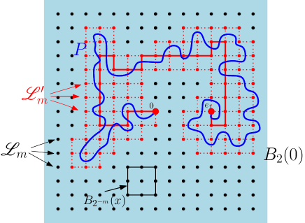
Let be a subset of defined as follows:
where represents the closure of . It follows that , and there exists a discrete path in connecting them. This is because for any considering the first exit time of from the box , we can find a vertex such that , and also enters the box . By doing this procedure iteratively, we obtain a discrete path in that connects and . Taking any path in connecting and , and applying the loop erasure procedure similar to (2.12), yields a self-avoiding path connecting and in . That is, there exists a self-avoiding path satisfying the properties that
| (3.19) | ||||
We now show that on the event , we have
| (3.20) |
This is because for each , the second property in (3.19) ensures that the path must cross the hypercubic shell . This segment has Euclidean length of at least . By the event , for some , we have:
Therefore, this segment has a -length of at least
| (3.21) |
Furthermore, each point on is contained in at most such hypercubic shells. Combining this fact with (3.21) and (3.18), we obtain (3.20).
Step 3: Modify the path on . Recall from (2.3) that . It follows that . We now construct a path on that closely follows the path and has typical -length. We call a vertex open if for all and
| (3.22) |
and closed otherwise. We assume that all the vertices in are open. Using the translation and rotational invariance and the scaling property from Lemma 2.5, we have
Combining this with the definition of from (3.2), we obtain that for all
| (3.23) | ||||
In particular, as approaches one, this probability also tends to one. Recalling the notation in Subsection 2.4, we similarly define open (or closed) (-)paths and (-)clusters on the rescaled lattice . Define the event
| (3.24) | ||||
Here, the diameter is associated with the graph distance on the rescaled lattice .
By the definition in (3.22), whether a vertex is open is determined by the field restricted to the domain . So, according to Lemma 2.6, for two subsets with graph distance at least , the statuses of the vertices in being open or closed are independent of the statuses of those within . Therefore, induces an -dependent measure on (where represents closed and represents open) with . As a result, we can apply the percolation result in Subsection 2.4. By using (3.23), Lemma 2.9, and Lemma 2.10 (with ), we can show the existence of such that when , the following inequality holds:
| (3.25) |
The last inequality is due to the fact that . From now on, we take
| (3.26) |
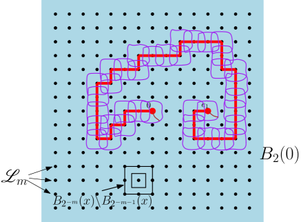
On the event , for each , there is no closed -cluster on that crosses the hypercubic shell 888For with , we consider the hypercubic shell instead. This ensures that for any under consideration, we have . or encloses . Therefore, by duality, there exists a unique open cluster on that encloses within the hypercubic shell . Furthermore, the open clusters corresponding to neighboring vertices on intersect, as illustrated in Figure 2. Since both and are contained in infinite open clusters, we can find open paths on see the brown curves in Figure 2. These paths connect and to their corresponding open clusters that enclose or , respectively.
By joining these open paths and clusters together, and applying the loop erasure procedure, we can construct a self-avoiding open path on that connects and , closely following the sequence . Let us denote the resulting path as . It satisfies the condition that for each :
| (3.27) |
Step 4: Concatenate the geodesic and upper bound the -length. In the final step, we join the geodesics between and for and upper bound its -length. Assume that
By using (3.27) and the definition of open vertices from (3.22), for each , there exists a piecewise continuously differentiable path that connects and and satisfies:
| (3.28) |
By concatenating the paths , we obtain a path that connects and within .
We now upper bound the -length of on the event . For each , by (3.27), we can choose such that
| (3.29) |
Since , we have
| (3.30) | ||||
By (3.29) and the event defined in (3.13), we obtain that there exists a constant (not depending on ) such that for all and ,
Combining this with (3.30) yields that
Combining this with (3.28) and (3.10), we further have
For each