Time-adaptive phase estimation
Abstract
Phase estimation is known to be a robust method for single-qubit gate calibration in quantum computers [1], while Bayesian estimation is widely used in devising optimal methods for learning in quantum systems [2]. We present Bayesian phase estimation methods that adaptively choose a control phase and the time of coherent evolution based on prior phase knowledge. In the presence of noise, we find near-optimal performance with respect to known theoretical bounds, and demonstrate some robustness of the estimates to noise that is not accounted for in the model of the estimator, making the methods suitable for calibrating operations in quantum computers. We determine the utility of control parameter values using functions of the prior probability of the phase that quantify expected knowledge gain either in terms of expected narrowing of the posterior or expected information gain. In particular, we find that by maximising the rate of expected gain we obtain phase estimates having standard deviation a factor of larger than the Heisenberg limit using a classical sequential strategy. The methods provide optimal solutions accounting for available prior knowledge and experimental imperfections with minimal effort from the user. The effect of many types of noise can be specified in the model of the measurement probabilities, and the rate of knowledge gain can easily be adjusted to account for times included in the measurement sequence other than the coherent evolution leading to the unknown phase, such as times required for state preparation or readout.
I Introduction
Phase estimation has found an increasing number of applications in metrology and quantum computing in recent years. Although resources are considered differently in these two settings [3, 4, 5], the methods of each have led to new applications in the other. In metrology, classical averaging limits to estimates with phase uncertainty scaling at best according to the standard quantum limit (SQL), , with the number of resources , while general strategies are fundamentally limited only by Heisenberg’s uncertainty principle and can obtain a improvement over the SQL reaching the so-called Heisenberg limit (HL), [6]. Entanglement was initially thought to be a key ingredient in schemes to reach Heisenberg scaling, [7], but when it was also found that the same scaling could be reached using sequentially prepared unentangled systems [8, 9, 10, 11, 12, 13, 14]111This is not necessarily true when noise is considered [88]., ideas from quantum computing [16, 17] soon led to new experimentally accessible metrology procedures with this scaling [18]. On the other hand, there have been several more recent proposals to use metrology methods to calibrate operations for quantum computing [19, 20, 21, 22, 1].
Many metrology proposals make use of a Bayesian approach to estimation which provides a natural framework to describe adaptive procedures, where the settings for future experiments are modified based on the results of previous measurements [23, 24, 25, 26, 27, 18, 28, 29, 30, 31]. While adaptive methods can lead to better performance, they are generally more complex than non-adaptive strategies and can also be more difficult to implement in some experiments. Remarkably, Higgins et al. found that they could reach near-optimal Heisenberg scaling using a non-adaptive procedure by optimising the number of measurements performed with different coherent applications of the unknown phase [32, 33].
While initial proposals like that of Higgins et al. [32] considered ideal settings with pure states and unitary operations, the role of noise and experimental imperfections has been increasingly studied over time [34]. This development has been both in the understanding of the fundamental limits to precision [35, 36, 37, 38, 39, 40, 41, 42, 43], and in devising better strategies to cope with non-ideal conditions, where the Bayesian framework with adaptive measurements has proved useful [44, 45, 46, 47, 48, 49, 50]. In some cases, adaptive methods have been used to design strategies better suited to the physics of particular experiments. In recent developments for the sensing of magnetic fields with NV centres, adaptive procedures were used to account for reduced visibility measurements [51, 52, 53, 54, 55, 56, 57, 58]222Readout can also be improved by adaptive methods [89, 90]. In many proposals the adaptive control acts on a phase that can be seen as an adjustment of the measurement basis, but the time of coherent interaction is chosen non-adaptively, e.g. as detailed in [32]. Since the interaction times proposed in [32] are optimised without noise, and thus may not be suited to experimental conditions, some experimenters perform optimisations using numerical simulations that include relevant noise in order to find interaction times better suited to their experiments[60, 61, 62, 53, 63]. Recently, Belliardo and Giovannetti [64] have analytically shown how to modify coherent interaction times in the non-adaptive procedure of Higgins et al. [32] to account for certain types of noise. Others have investigated the possibility of also choosing the interaction time, or equivalently, in the case of some optical measurements, the size of a so-called N00N-state [33]333This is an example where entanglement can be used to convert temporal resources into spacial resources [11]., adaptively: initially in proposals without noise [27, 33], or with mixed-state quantum computation [28], and later in proposals using numerical algorithms that can also account for noise and imperfections [66, 67, 68, 57, 69].
Commonly the performance of a strategy is only considered in the asymptotic regime, when the number of resources (i.e. number of physical systems and total estimation time) approaches infinity. Many experiments, however, could benefit from strategies that are optimised for finite resources. Phase estimation in metrology is typically studied in two settings. In one setting, often referred to as local, the goal is to achieve optimal sensitivity to phase fluctuations from an a priori known phase . In the other setting, referred to as global, it is assumed that there is initially no a priori knowledge of the phase [47]. While the amount of a priori knowledge of the phase is not relevant in the asymptotic regime, it can significantly change the optimal estimation strategies for finite estimation times [70]. Therefore, it is useful to have methods that can account for arbitrary a priori phase knowledge.
In addition, the coherent interaction time in many proposals is optimised under the assumption that this time dominates the experiment time. While this is true in the asymptotic regime, many experiments may not reach this regime for all or at least a significant portion of the estimation time [54]. An extreme example is found in GaAs quantum dots where the measurement time is several orders of magnitude longer than the coherent evolution [71]; here the authors show an exponential improvement in the mean-square error (MSE) of parameter estimation by adaptively choosing the time of coherent evolution.
In this paper we present time-adaptive phase estimation (TAPE), a method that allows for the adaptive optimisation of the coherent interaction time and a control phase to be adjusted to the resources of the experiment. TAPE can provide strategies optimised both when the experiment time is proportional to the time of coherent interaction, and when the experiment time is proportional to the number of measurements; the method also allows for any resource allocation in between these two extreme cases. In addition TAPE can provide optimal strategies for arbitrary a priori knowledge of the phase, because the choice of measurement settings depends only on the prior knowledge of the phase after the last measurement, and not on any record of previous measurements. In contrast to earlier works investigating similar adaptive procedures [27, 33], we use a more general form for the measurement probabilities so that we can account for many types of noise or imperfections.
We propose and analyse several different objective functions for the adaptive parameter selection that lead to near-optimal performance with respect to known theoretical bounds, with and without noise. When the experiment time is proportional to the time of coherent interaction we reach uncertainties in the phase estimates that are a factor of larger than the HL. In addition, we find that TAPE is quite robust to errors that are not accounted for in the model of the estimator. This demonstrates that, similarly to proposals like robust phase estimation [1], our methods are well-suited to calibration of single-qubit operations in the context of quantum computing.
TAPE uses a numerical representation of the phase knowledge as a Fourier series that can easily describe arbitrary prior knowledge, at the possible expense of increased computation. Since the complexity of the Fourier representation (i.e. number of coefficients to track in memory) increases with phase knowledge, the computation time required for adaptive control of experimental parameters may become too large for some practical applications. To tackle this limitation we propose a method that reduces the interval over which the Fourier representation of the phase is used. This can significantly reduce the required memory and time of computation.
II Bayesian estimation
The evolution and measurement for a single step of sequential phase estimation can be described by the quantum circuit in Fig. 1 [72]
@C=1em @R=.7em
\lstick— 0 ⟩ \gateH \ctrl1 \gateR_z(-α) \gateH \meter\cw
\lstick— ϕ ⟩ \qw\gateU^k \qw\qw\qw\qw
where is the Hadamard gate, with Pauli operator is a z-rotation, and is a control phase to be optimised. with an eigenstate of the unitary with unknown phase . determines the number of applications of the unitary evolution. The parameters and will be chosen adaptively for each measurement as detailed in section III. We denote the possible measurement outcomes at step by , and in order to describe a range of noise or measurement errors [54], we assume the outcome to occur with probability
| (1) |
where allow respectively for the description of asymmetry and reduced contrast in the measurement444While describes a reduced probability for the outcome , the reverse situation can always be described by relabelling the outcomes.. The subscript of indicates that these values can generally depend on . Since the outcome and the control parameters and depend on we should really denote them but we omit the subscripts for simplicity of notation.
As in [27, 33, 51] we use a Fourier series to write the probability density describing our knowledge of the phase at step
| (2) |
Given prior knowledge and measurement outcome , we update our state of knowledge using Bayes’ theorem
| (3) |
where
is the posterior probability of outcome . Equation (3) specifies how to modify the coefficients given the measurement outcome.
We choose to use the estimator
| (4) |
A nice feature of the Fourier series representation for is that the estimator (4) depends only on one coefficient. Given an estimate of (in general now, not necessarily given by (4)), we quantify the uncertainty in by the square root of the Holevo variance [74]:
| (5) |
where is the sharpness and the angular brackets indicate an average over the estimates . If the estimate is biased, one can use instead, where is the value of the correct system phase [33]. In [26] the authors show that the estimator (4) minimises the Holevo variance (5).
III Adaptive procedures
In the previous section we have described how in general to use Bayes’ theorem to update our knowledge of the phase given the measurement outcomes, and how to obtain an estimate from the density at step . The task of achieving minimal uncertainty in the estimates obtained from (4) is then dependent on the choices of the values of the control phase and the number of applications of . In a sequential procedure, the state coherently evolves according to for a time proportional to , so that the choice of corresponds to choosing the time of coherent evolution. In the following we will assume such a sequential procedure, but we note that the results can also be applied in the case of some parallel procedures by using entanglement.
Given prior knowledge at step we look to choose the optimal control phase for a given value of by maximising a function of , , and that quantifies the expected knowledge gain from the next measurement. One might then expect that the optimal choice of can be determined by maximising the expected knowledge gain over all possible values of . This can be a good choice when the evolution time of is negligible compared to other times in the experiment, as in the example of GaAs quantum dots mentioned above [71]. But in general experiments with different values of require different resources in terms of execution time, so that the expected knowledge gains for different values of are not directly comparable555Even more generally, which resources are valuable depends on the setting and what the experimenter wants to optimise. e.g. they may have a restricted number of qubits to measure, so that number of measurements becomes the relevant resource. In this sense it is useful to have a method where the optimisation can be adjusted by the experimenter to describe best how they value their resources..
In [27, 33], the authors studied a method where the value of is chosen adaptively. In [27], corresponds to the number of photons in a N00N state, however as shown for the noiseless case in [33] the sequential procedure we discuss here is mathematically equivalent. This equivalence also holds under certain types of noise [13, 14]. Physically these two procedures are different but they are connected by the use of entanglement to convert between temporal and spatial resources [11].
In the case that the experiment time is proportional to , the relevant resource is the number of applications of . This way of considering resources, which is typically chosen in quantum metrology, is considered in [27, 33]. In these works the authors calculate the expected (differential) entropy 666The differential entropy is the entropy of a continuous random variable, but it lacks some important properties of the Shannon entropy for discrete random variables. See e.g. [91], chapter 8. In this manuscript we will usually write simply “entropy” when referring to the differential entropy. of the posterior after the next measurement using a Gaussian approximation. Motivated by the resource dependence on they choose the value of that minimises the expected entropy divided by . Here refers to the total number of resources used since the beginning of the estimation sequence, where an initially uniform prior is assumed (no prior knowledge of the phase). Since this method requires knowing assuming an initially uniform prior and because the priors in the later stages of the estimation must be approximately Gaussian, it is not well suited to incorporating arbitrary prior knowledge. Moreover, the approach of dividing the entropy by is based on scaling of the uncertainty in the phase that is only valid without noise.
Here we study two different methods for adaptively choosing that have the following features:
-
1.
The resource dependence on is adjustable so that it can be chosen to match a given experiment. Since we consider sequential procedures, we take the resource requirement for performing an experiment with a particular value of to be the time required to perform that experiment.
-
2.
The choice of for a given measurement is determined only by the prior probability density at that step of the estimation sequence.
-
3.
The methods can be applied to different functions quantifying the expected knowledge gain associated with a particular choice of . We study two such possible functions possessing different benefits: the expected sharpness gain and the expected (differential) entropy gain.
In the following we show how to calculate these two functions quantifying expected knowledge gain exactly; with the exact expressions in hand these functions can be computed for any prior, not only Gaussian. The expected knowledge gains are calculated from expressions that can describe experiments with noise. This allows the methods to determine good phase estimation procedures for noisy experiments, as well as in the noise-free case.
III.1 Expected knowledge gain
Given prior knowledge at step , one might expect that in order to minimise the Holevo variance of the estimates (equation (5)) at step , a good strategy can be to choose the control phase that minimises the expected Holevo variance of the posterior Bayesian probability density for the next measurement. However, it is shown in [26, 33] that in order to minimise the Holevo variance of the estimates one should choose to maximise the expected sharpness of the posterior Bayesian probability density for the next measurement
where we denote the sharpness of by
| (6) |
Similarly to the estimate (4), a nice feature of the Fourier series representation for is that the sharpness (6) depends only on a single Fourier coefficient. Maximising the expected sharpness of for the next measurement is a good strategy since the sharpness of the estimates can be written as the average of over possible measurement records; maximising the sharpness of the estimates is equivalent to minimising the Holevo variance of the estimates [33]. We note that the average of over possible measurement records considered in [33] assumes a uniform prior at the beginning of the estimation sequence, and this strategy may be less optimal for other priors.
In order to evaluate the best strategy for the measurement at step , we define the expected sharpness gain as
| (7) |
rather than working with the expected sharpness of the posterior directly. The reason for working with the gain will become clear later on when we consider gain rates. Similarly, we define the expected entropy gain for the probability density at step ,
| (8) |
where is the differential entropy of ,
We note that can be seen as the expected information gain from the next measurement. It can be rewritten as (see Supplemental Material, section S.V)
where we denoted , for short, and is the Kullback-Leibler divergence of the posterior from the prior [77, 78]. In ref. [50] the authors show that maximising expected entropy gain maximises the likelihood of estimating the true phase. In terms of the coefficients of the prior, this can be computed by an expression of the form
| (9) |
The -dependent coefficients and are generally also functions of and . Since our knowledge after a finite number of measurements is always described by a finite Fourier series, the sum over is always finite. The derivation of this expression as well as the exact expressions for , , and are given in the Supplemental Material, section S.V.
Before discussing in detail how to use the expected gains to choose we discuss the choice of the control phase and compare the benefits of using sharpness to quantify expected knowledge gain versus entropy. For both methods described in section III.2 below, computing the expected gain for a given value of always involves an optimisation of the control phase for that particular -value. An example prior is shown in figure 2 and the values of the expected entropy and sharpness gains for the next measurement are plotted for . The expected entropy gain increases significantly from to while the increase for larger -values is smaller. The expected sharpness gain also increases significantly from to , but contrary to the expected entropy gain, decreases for , and becomes zero for . This is because as increases, it is increasingly likely that the posterior will have multiple peaks. When the effect of the measurement leads to a posterior density that is split into multiple peaks with an envelope similar to the prior density, so that the sharpness is unchanged. Conversely, the entropy still increases when the probability density is split into multiple peaks, so that the expected entropy gain is large for all values of .
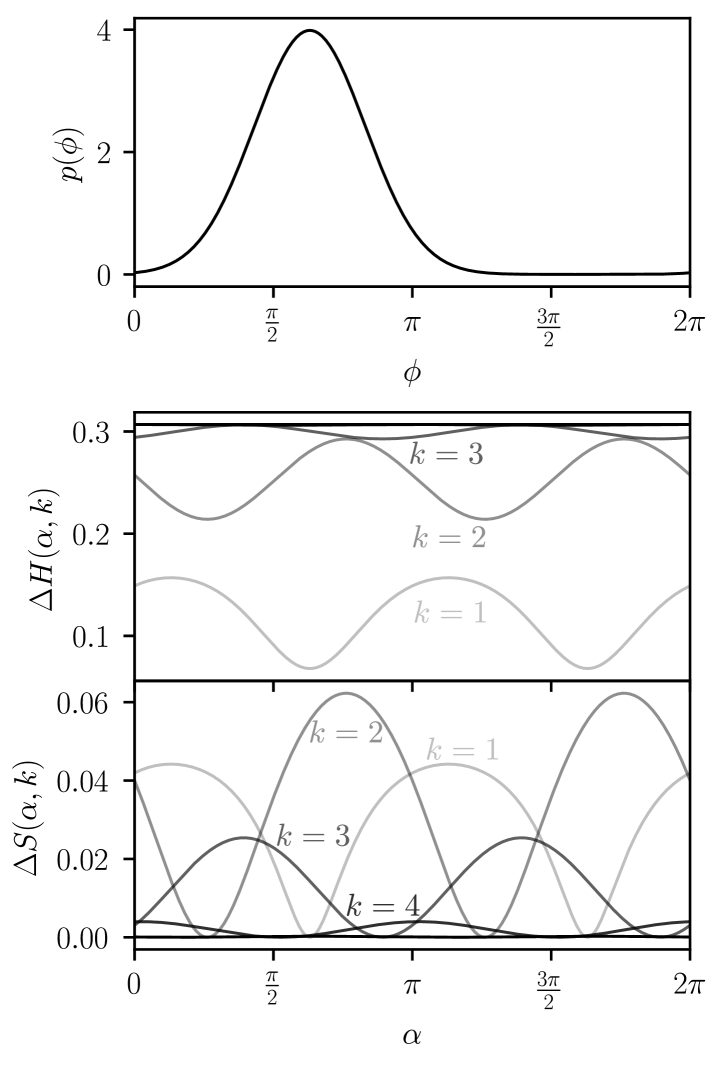
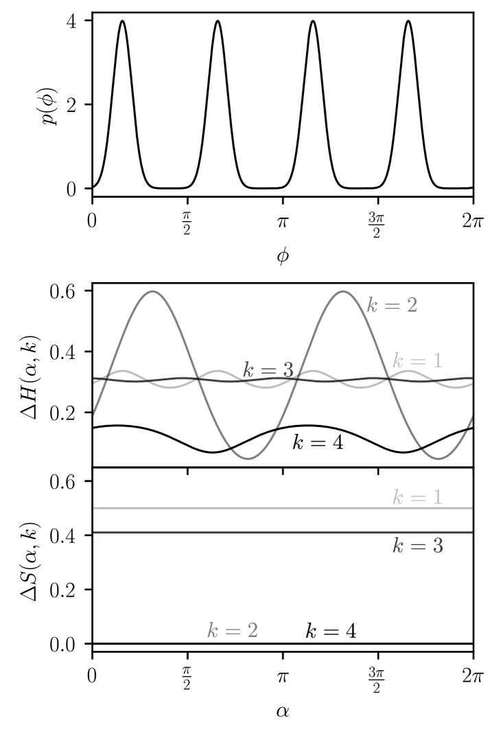
These differences between the entropy and the sharpness make them useful for different purposes. Maximising the expected sharpness gain is useful to ensure that the probability density has a single peak – this is important for obtaining an accurate estimate of the phase. On the other hand, the entropy allows to quantify good strategies when there are multiple peaks in . In figure 3 we plot a prior with four peaks along with the expected entropy and sharpness gains to illustrate these differences. We see that the maximum entropy gain corresponds to a measurement with that will eliminate two of the peaks in with high probability. In contrast, the expected sharpness gain for is zero because the density with either four or two equally spaced peaks has zero sharpness, meaning that the strategy of eliminating two peaks is not quantified by the sharpness. The expected sharpness gain in this case is non-zero only for odd values of since they will lead to a narrowing of the envelope of . The entropy quantifies strategies that sharpen the overall envelope (), the strategy of eliminating two peaks (), and the strategy of sharpening the individual peaks ().
III.2 Choosing
We now describe the two methods for choosing . As noted above, if experiments with different values of require different amounts of resources, comparing the expected knowledge gain for different does not directly provide a means for choosing .
Let be a vector of possible -values for the next measurements, and let be the vector of corresponding times; i.e. is the time required to perform an experiment with . The methods for choosing take the vectors and as input. The value of the expected gain used by these methods is the maximum over possible values of .
III.2.1 Multi-step gain method
The first method we study for the adaptive choice of is based on the following idea: if we compute the expected gain for more than one measurement we can compare the expected knowledge gain for different sequences of measurements that take the same total time. Comparing many possible -values in this way will generally lead to an expensive optimisation since there can be many measurement sequences that take the same total time, and because the complexity of computing the expected knowledge gain grows exponentially with the number of measurements (also see the Supplemental Material, section S.III). Therefore we devise a technique which allows us to compare only a few -values at a time.
The following example illustrates how this method proceeds. Suppose the amount of resources per -value is proportional to () and we restrict the choice of to the set . We can then compute the expected knowledge gain for performing two measurements with versus the gain for performing one measurement with . If the former is greater, we perform an experiment with . Otherwise, we can compute the expected knowledge gain for performing two measurements with versus that for performing one measurement with . If the former is greater, we perform an experiment with , and so on. Note that calculating the expected gain for multiple measurements requires optimising one control phase for each measurement. This optimisation is performed sequentially starting with the first measurement. A detailed description is given in the Supplemental Material, section S.III.
In this example we see that we need only compute the expected knowledge gain for one or two measurements and for only a few possible sequences of measurements. We expect this to converge to a locally optimal choice of . This method for choosing can be generalised to other possible input vectors and using an algorithm which is given in the Supplemental Material, section S.III. It works with vectors and sorted in increasing order, under the assumption that implies , and restricted to . In this general algorithm we restrict the computation of expected knowledge gain to at most 5 measurements to prevent the computation from becoming too expensive. To allow for general inputs and under this restriction, we in general compare sequences that require only approximately the same time. The detailed method is described by algorithm S.5 in the Supplemental Material, section S.III.
III.2.2 Gain rate method
The second method we study for choosing uses the rate of expected knowledge gain. A similar idea has been used recently to estimate decoherence timescales in a qubit [79]. We compute a vector of expected knowledge gain where corresponds to the expected knowledge gain for performing a single measurement with , computed using either (7) or (9) depending on the choice of gain function. We then calculate the vector of expected rate of knowledge gain (elementwise division), and choose the with . The value of may be found by performing a brute force search over -values. Since we use a computation that runs in series, the brute force search can take too long for many practical implementations, and we reduce the computation by performing a Fibonacci search [80] to find a good value of . Since the computation of any element of can be performed independently, a brute force search could be performed by computing the gain rate for each -value in parallel. Since the brute force search is expected to lead to slightly better performance than the Fibonacci search we use here, it could be considered for future implementations. Overall, the gain rate method has the advantage of being simpler and computationally cheaper than the multi-step method.
IV Numerical representations
The representation of phase knowledge using the Fourier series (2) means that the number of non-zero coefficients to keep track of increases with our knowledge of the phase. If the number of non-zero coefficients at step is , the computation for the Bayesian update (3) requires calculating new coefficients. Considering the case that we start with a uniform probability density, we initially have in (2). After performing some measurements with applications of in total, the last update will require calculating non-zero coefficients.
If we are in a situation which results in Heisenberg scaling, then . If the scaling of is slower than Heisenberg scaling, then it follows from (3) that the number of coefficients after reaching a given value of will be greater than for Heisenberg scaling. However, if we assume a probability density which on average preserves its functional form (i.e. the overall shape stays the same and only the width changes) as estimation proceeds and decreases, then from standard Fourier analysis should scale as . This follows from the fact that we expect the square root of the Holevo variance of the Bayesian probability density, , to scale in the same way as with . This suggests that when we converge more slowly than Heisenberg scaling, the description of obtained from (3) uses disproportionately many non-zero coefficients and becomes inefficient. For this case, we should seek a good representation of with fewer coefficients to minimise computational overhead. In this sense we can expect that it should be possible for the number of coefficients to be inversely proportional to the uncertainty, , even if we do not have Heisenberg scaling.
The computation for adaptively choosing and scales more favourably with than the Bayesian update. Computing the expected sharpness gain (7) does not scale with the total number of coefficients , while the expected entropy gain (9) scales as . Since we expect the optimal value of to increase with (in the noise-free case), there may exist algorithms, offering a complexity independent of , for choosing such that the expected entropy gain typically is maximised.
The practicality of using TAPE depends on the possibility of computing the Bayesian update and choice of control parameters ( and ) in a time shorter or equal to the time it takes to run the next measurement. Since the update computation time scales linearly with , it will become longer than the measurement time for sufficiently large . In the asymptotic limit when , the average measurement time, proportional to for sequential procedures, will also scale linearly with if we have Heisenberg scaling. If the slope of the linear increase in computation time is less than that of the measurement time, the computation will remain shorter than the measurement time on average for all . However, this may not be the case for many experiments where TAPE could otherwise be useful, for example if decoherence prevents large -value measurements from giving phase information, or if TAPE is used for parallel procedures. In these cases it is beneficial to find methods that reduce the time of computation. One approach is to change representation from a truncated Fourier series to another function such as a Gaussian which is described by a number of parameters that is independent of [81]. Here we propose an alternative method that allows the truncated Fourier series representation to be used for arbitrarily large while ensuring that the number of coefficients needed in the series scales much slower than . This way all the procedures of sections II and III can still be used for large with minimal changes, and the user is also free to adjust the generality of the description of versus computational overhead as suits their purposes.
Given a probability density , we define a contraction of as , such that for and otherwise. We refer to as the magnification, to as the offset, and we represent as a truncated Fourier series. Thus, by representing the density as a contraction we use the truncated Fourier series representation for and assume that for values of outside this interval. We are effectively “zooming in” on a region around the expected value of and assuming that the probability of outside this region is negligible. Given a contraction where has coefficients we can calculate a new contraction , a multiple of with as
| (10) | ||||
| (11) |
where .
By using the truncated Fourier series on a reduced interval of size , a contraction of (with coefficients) uses only coefficients. The assumption that outside the interval is often false with finite probability. However by performing more measurements this probability can always be reduced arbitrarily while increasing the number of coefficients . Once this probability is small enough for the given application we can make contractions to ensure that the number of coefficients no longer exceeds . Thus, with this method we must balance the probability that a contraction fails to represent the estimated phase against the maximum computation time per measurement.
In the Supplemental Material, section S.IV, we show that under the assumption of a Gaussian probability density , using contractions reduces the number of Fourier coefficients required by , while keeping the probability that outside the interval below a constant value (which can be chosen to be arbitrarily small). In general, the computational complexity will depend on the particular functional form of , but the Gaussian case demonstrates that the method can sometimes greatly reduce computation. If a much poorer complexity is found when faster computation is needed, it could be helpful to modify the adaptive strategy for choosing and such that becomes closer to a Gaussian before each contraction is performed.
The expected sharpness or entropy gain relations (7) and (9) can be used for the contracted Fourier series representation with the replacement , although the values of the expected sharpness gain in that case will not correspond to those for the full density 777Although the differential entropy is not invariant when changing the scale, the differential entropy gain is.. However the control parameters that achieve the maximum gain for the contraction can still be used to determine the values to use for the next measurement. Denoting the optimal control phase thus obtained as and the optimal number of applications of as , then the corresponding values to use for the un-contracted density can be calculated as , . In this way we can use contractions to reduce the time not only for the update computation but also for the search of optimal parameters and using the expected entropy gain 888this also works when using sharpness gain, but there is no speedup.
V Simulation results
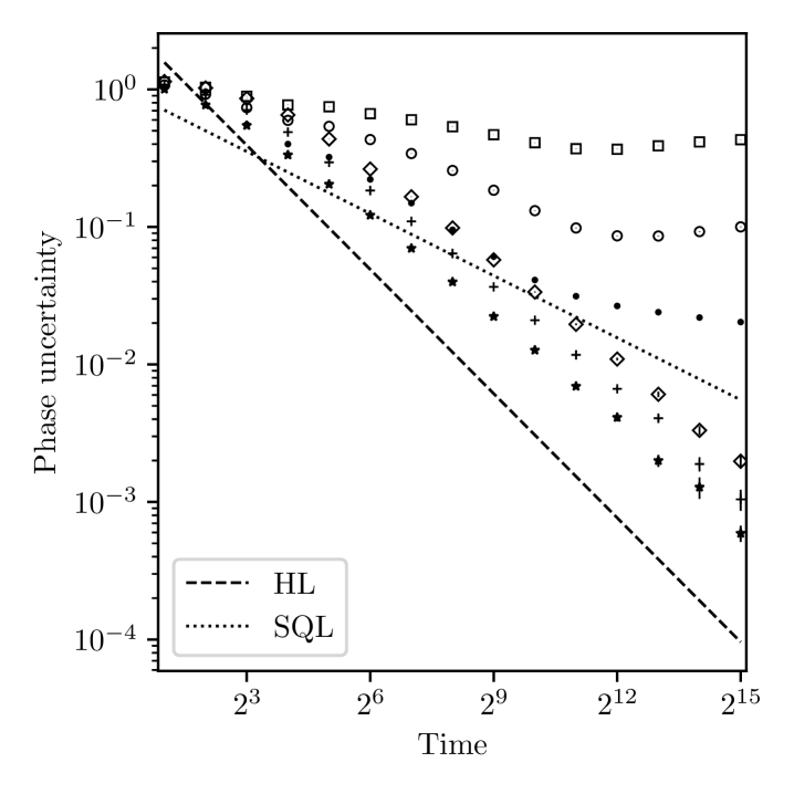
In order to characterise the performance of the methods considered above we study the results of numerical simulations. We focus on estimation starting from a uniform prior (initially no information about the phase), though we note that our methods are also well-suited to any prior that can be well-represented with a Fourier series and the contractions described in section IV, given available computational resources and particular timing requirements of an experiment. We first consider the case of noise-free quantum metrology. In this context the time of the measurement is assumed to be proportional to the number of applications of the unitary evolution ; in the following we set the time of to 1 so that the time of a single measurement is equal to . In this case, the number of resources in the SQL, , and HL, , is the total number of applications of in the estimation procedure, and is equal to the total estimation time.
In figure 4 we plot the uncertainty in the phase estimates resulting from repeating the estimation procedure with randomly chosen values for the system phase 999The performance of estimation may be dependent on the system phase when starting from a uniform prior if the control phase for the first measurement is fixed (e.g. ). By choosing a random control phase for the first measurement, the performance is the same for any value of the system phase. Thus, our results can also be interpreted as the performance for any particular value of the system phase assuming a random control phase is used in the first measurement.. More specifically, we plot the uncertainty multiplied by total estimation time for which any phase estimation reaching HS results in a constant value independent of estimation time; for the HL, the constant value is . The uncertainty in the phase estimates is calculated according to equation (5), where the sharpness is calculated as for a true system phase , and the expectation value is approximated as an average over simulations. This choice can only lead to larger uncertainty values than the usual sharpness, , since . For the results in figure 4 we find , which shows that the estimator is unbiased and either choice of sharpness measure leads to essentially the same values for the uncertainty. Nevertheless, in all simulation results presented in this manuscript we have calculated the phase uncertainty using .
For the multi-step (gain rate) method, each plotted point is calculated from () realisations of estimation. We compare four adaptive methods for the choice of control parameters and . For the multi-step method we plot separately the results of maximising either the expected sharpness gain (7) or the expected entropy gain (9) for total estimation times . For the gain rate method we plot the results of maximising the expected sharpness gain (7) to determine the choices of and , but we find that maximising the expected entropy gain (9) performs worse (not shown), which is due to the properties of entropy mentioned in section III.1. We also note that when maximising the expected entropy gain only, we tend to obtain very accurate estimates with a small number of outliers that significantly increase the phase uncertainty.
Instead of studying further the gain rate method maximising only expected entropy gain, we plot the result of a hybrid strategy in which the choices of and are determined using the expected entropy gain for at most the first half of the total estimation time, and the expected sharpness gain is used for the remaining time. This approach is motivated by the fact that although maximising ones information about the phase is desired, obtaining a precise estimate for the phase additionally requires a narrow probability density . Since multi-peak density functions can have the same entropy as single-peak functions with a broader peak, maximising the entropy doesn’t necessarily lead to a narrow density. We choose the hybrid method to study the performance of strategies that maximise the information gain, while still ensuring a narrow density that is required for accurate phase estimation.
As shown by Gutiérrez-Rubio et al. [50], maximising the entropy gain leads to the maximum likelihood of estimating the correct system phase. Another way to understand the drawback of maximising the entropy gain only, is that maximising the likelihood of estimating the system phase does not generally minimise , which depends on the entire distribution of phase estimates, call it , rather than the value at a single point. Note that if one could maximise expected gain over an entire measurement sequence used for estimation, maximising the expected sharpness gain should minimise [33]. Since we perform the optimisation only for the next measurement, it becomes interesting to study the hybrid method.
The two plotted methods based on gain rate are for total estimation times , and all methods make use of contractions (section IV) to reduce computation times; if the square root of the Holevo variance of the phase density, is less than , where is the current magnification, then we perform at least one measurement using parameters that maximise the expected sharpness gain, and then we perform a contraction with . The additional measurement to maximise the expected sharpness gain is used in the hybrid method, and multi-step method maximising entropy to reduce the probability of the system phase being outside the reduced interval over which the Fourier series representation of the phase knowledge is used in the contraction. Since -values are chosen adaptively, a sequence of optimal choices does not generally lead to the total times we choose to plot in figure 4. For the simulations plotted we therefore always restrict the optimisation over to values less than or equal to the total remaining time. For this reason we have performed simulations for each plotted point independently of the other points for different total times.
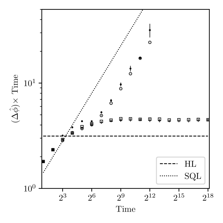
The results in figure 4 show that all methods perform better than the SQL. The gain rate method using sharpness gain or the hybrid method perform best, and we fit the results for total estimation times from to with a functional form . The values of and obtained from the fits are summarised in table 1. The hybrid method clearly reaches HS (), while the method maximising sharpness only is extremely close to HS, and both methods are close to the theoretically lowest achievable uncertainty for the values simulated. In particular, the uncertainty for a total time of (i.e. the longest time simulated) is a factor of from the HL when maximising sharpness gain only. For the same total time the hybrid method reaches an uncertainty within a factor of from the HL.
| Method | ||
|---|---|---|
| sharpening | ||
| hybrid |
We attribute the poorer performance of the multi-step method to the fact that the compared gains require only approximately equal time and to the fact that only a local optimum is used (see Supplemental Material, section S.III). Although we expect the performance could be improved by starting the search at a -value dependent on the Holevo variance of the prior (cheap to compute) and additionally using a “search down” method analogous to algorithm S.4 (see Supplemental Material, section S.III), we choose rather to focus on the gain rate method since it demonstrates near-optimal performance in addition to being simpler and computationally more efficient.
In the Supplemental Material, section S.I, we have also compared the multi-step and gain rate methods in the case where we allow only the subset of -values: . In this case the gains compared by the multi-step method require exactly the same time, and the method performs similarly to the gain rate method. However even in this situation the multi-step method at best performs similarly to the hybrid method using the gain rate. For completeness, we have also simulated the gain rate methods studied here when a brute force search for is used rather than a Fibonacci search. In that case the hybrid method performs best reaching an uncertainty within of the HL. A summary of simulation results for the best performing methods we have studied is given in table S.1 in the Supplemental Material, section S.I.
In figure 5 we consider the performance of the methods using the gain rate when the measurement time is independent of . This situation describes the limit where the time required to perform the unitary evolution is negligible compared to other times in the experiment such as state preparation and readout. In this case the total time is equal to the number of measurements. We plot methods based on maximising either sharpness gain or entropy gain as well as a hybrid method, as in figure 4. In addition we compare the case where the gain maximisation is based on the correct rate in this context, i.e. where (so ), with the usual case in metrology: . We plot the mean error resulting from realisations of estimation from 1 to 40 measurements.

The results in figure 5 show that the strategies using the correct rate () outperform those optimised for the usual metrology setting with . In this case we find that the method that maximises the expected entropy gain performs best while that maximising expected sharpness gives the lowest accuracy in phase estimation; the hybrid method has a performance in between the two. We fit the results from to measurements with an exponential decay . The values of the fitted parameters and for each of the plotted curves in figure 5 are listed in table 2.
| Method | ||
|---|---|---|
| sharpening (M) | ||
| hybrid (M) | ||
| entropy (M) | ||
| sharpening | ||
| hybrid | ||
| entropy |
Although the performance is better when the correct rate is used, the improvement is not dramatic. This is perhaps not surprising since the quantum phase estimation algorithm (QPEA) [85, 72] is known to be optimal even when the number of applications of is not the relevant resource (indeed this is also the case in the setting of quantum computation) [3, 4]. Methods based on QPEA also lead to Heisenberg scaling in the context of quantum metrology [33]; that is, estimation procedures using similar allocation of per measurement have been shown to be optimal in both settings. Nevertheless, we see that in the case of the single-step optimisation we perform for sequential strategies we can obtain a slight improvement by using the appropriate rate in the optimisation. In this setting we attribute the better performance when maximising the information gain rather than the sharpness gain to the fact that higher -values are cheap compared to the metrology setting, allowing strategies that are better quantified by the richer nature of the entropy.
For the remaining simulations we return to the metrology setting where since in this context we can compare performance with known theoretical bounds. In particular, we study the performance in the presence of noise.
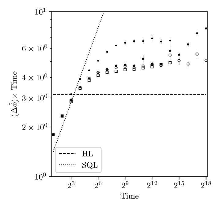
In figure 6 we model a system with dephasing. We assume perfectly prepared states, and , the Pauli-z operator. After each application of we additionally apply a dephasing channel described by the Kraus operators , . At the end we perform the measurement in the x-basis. In this case it is possible to have Heisenberg scaling only initially while increasing is beneficial, but as is increased dephasing eventually reduces the information available by the measurement and we are restricted to scaling. The ultimate bound on precision can then be expressed as , where is a prefactor depending on the noise channel. In the case of dephasing this prefactor has been shown to be equal to at least (but it is not known if this bound is tight) [39]. In figure 6 we consider the case where ; the bound is also plotted. As before we simulate the gain rate method for sharpness gain, entropy gain, and the hybrid case described above. We compare these three methods when no decoherence is accounted for in the estimator model ( in equation (1)) and when the decoherence rate is already known (). We plot the phase uncertainties calculated from realisations of the estimation starting from a uniform prior and system phase chosen uniformly at random.
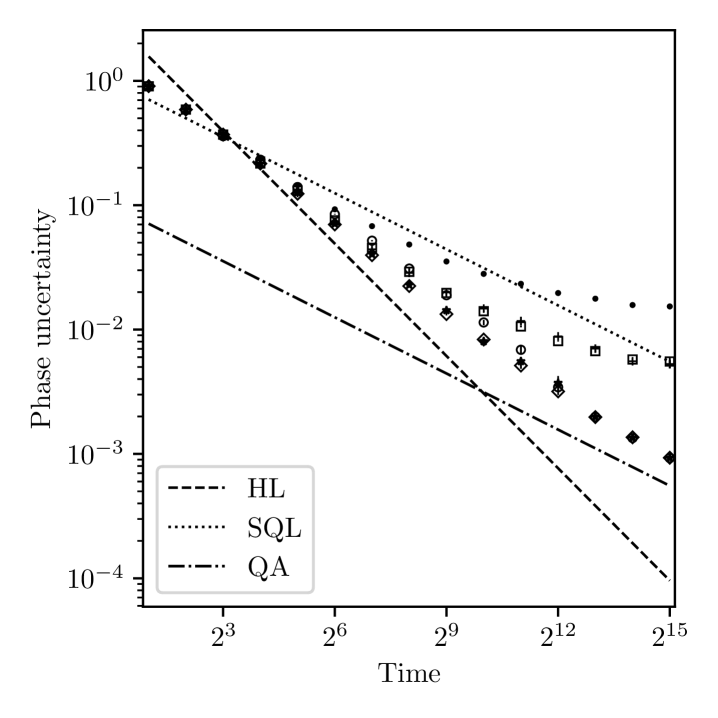
When decoherence is not accounted for in the estimator model, maximising the entropy leads to the poorest performance since this chooses larger -values for which the system decoheres, leading to reduced information in the measurement. For all methods that do not account for decoherence in the model, estimation works initially, but as is increased decoherence eventually introduces large random errors in the estimates. When decoherence is accounted for in the model we find that all methods perform well. When sufficiently many resources are used the method that maximises the rate of entropy gain performs similarly to the other methods. This can be explained by the fact that decoherence eventually limits the -values chosen by the strategy and the density is far less likely to have multiple peaks. We find that when the decoherence is accounted for, the performance after a total estimation time of is within of the theoretical bound when maximising the expected entropy gain, when maximising the expected sharpness gain, and for the hybrid method. Our methods could also be combined with an optimised estimation of decoherence timescales as proposed by Arshad et al. [79].
The results in figure 6 demonstrate some robustness of the estimation methods to errors not accounted for in the model. In figure 7 we present the results of a last set of simulations to examine further the robustness of the methods. In this case we assume perfectly prepared states and . After the applications of we apply a bit-flip channel with Kraus operators , , Pauli-x,y, followed by spontaneous emission with Kraus operators
We choose to set , and simulate the hybrid gain rate method with . For each value of we simulate estimation using an estimator model with () and without () errors included.
We see that when errors are included in the model the phase uncertainty is significantly larger than in the noise-free case, but we still retain better than classical scaling for longer estimation times. We fit the phase uncertainty with a functional form , with fit parameters and . By fitting subsets of points we see that tends to increase for longer times, but we would need to simulate further to see if HS is eventually reached. When errors are not included in the model, only the case performs similarly to the SQL initially, while for larger errors the performance drops significantly. We see also that for longer estimation times the lack of errors in the model can prevent further reduction of the phase uncertainty. This suggests that it may be better to restrict to lower -values in the presence of large unknown errors. Overall, these results demonstrate robustness of the method to large errors indicating that TAPE can also be useful for calibration of quantum systems, e.g. for quantum computing, as considered in ref. [1].
In the noise-free case we find average computation times are for the computation required for a single shot using a standard PC (CPU model: Intel(R) Core(TM) i7-8565U CPU @ 1.80GHz) without any parallel computation. When noise is included in the model we find that the maximisation of expected knowledge gain can take a time up to for the entropy gain, and when maximising the expected sharpness gain. This makes the method suitable for trapped ion or neutral atom based quantum computing systems where the time of a single shot is typically a few milliseconds. Since the computation of expected knowledge gain for each -value could be performed in parallel it may be possible to obtain sufficient speedups for some applications in superconducting circuits or NV centres. Further speedups may also be possible when maximising the expected sharpness gain if the optimal value of where determined analytically. An alternative approach to achieve faster computation with the implementation we use here is to restrict measurements to use only a subset of possible -values; a further discussion can be found in the Supplemental Material, section S.I.
For experimental systems with sufficiently low measurement rates, TAPE thus provides a near-optimal and very flexible method for phase estimation. In the metrology setting without noise, the best performance we know of for phase estimation using a classical sequential strategy is the adaptive method of Higgins et al. that is inspired by QPEA from quantum computing [18, 4]. Their adaptive method reaches a phase uncertainty (as quantified by the square root of the Holevo variance of the estimates) a factor of larger than the HL, while they have later devised a non-adaptive method, also inspired by QPEA, that performs similarly, demonstrating uncertainty less than a factor of larger the HL [32, 33]. The latter non-adaptive method has also been shown to be a robust method for calibrating single-qubit gates for quantum computation [1]. Non-classical strategies for phase estimation reaching lower uncertainty estimates are known, as e.g. the method of Pezzè and Smerzi [86, 87] which provides phase estimates with uncertainty 1.27 larger than the HL. However, classical sequential strategies are best suited to single-qubit gate calibration. In the metrology setting we have found that TAPE reaches an uncertainty that is a factor of larger than the HL using the hybrid method, demonstrating similar or better performance to known methods. The results presented in figures 6 and 7 also show significant robustness to errors, demonstrating that TAPE can be a good method for calibrating single-qubit operations.
In contrast to algorithms inspired by QPEA where a predetermined number of measurements is performed for values of , TAPE chooses the time of phase evolution (i.e. the -value) adaptively. For the non-adaptive method that is used for robust phase estimation [1, 32], the number of measurements for each -value is optimised beforehand for a given total number of phase applications assuming no prior knowledge of the phase. If noise is present the optimisation needs to be modified as shown in [64]. But as noted therein, the noise models they consider “are to be thought more as toy models” that “capture some of the key features of those scenarios”. Depending on the type of noise present in a given experiment a further analysis and optimisation of the number of measurements to perform with each -value will be required to minimise the phase uncertainty. By using the general form for the measurement probabilities (1), TAPE allows for the description of a wide range of noise to be included in the model of the estimator and directly provides near-optimal phase estimation procedures by accounting for the modelled noise in the optimisation for the control parameters and .
In addition, TAPE allows the exact experiment times to be easily included in the optimisation for the adaptive choice of -value. This is very convenient for experiments where state preparation and readout times cannot be neglected in comparison to the time required to apply the unknown phase. Using the QPEA inspired methods above, a further optimisation of the number of measurements with each -value would otherwise be needed to minimise the phase uncertainty.
In the QPEA inspired methods above, the value of to use for a particular step in the estimation sequence requires knowing how many measurements have been performed so far with each -value. In TAPE, once the model of the noise is specified (by setting the values ), and the experiment times required for each -value are set, the values of the control parameters and are determined using only the current prior knowledge density . This makes it easy to apply TAPE in situations where some prior knowledge may be available. As an example suppose we would like to use phase estimation for calibrating single-qubit operations on a quantum computer where internal parameters of the device can drift over time. One could use either TAPE or a QPEA inspired method to initially estimate parameters. However, it would be easy to include the drift rate in the model of the phase knowledge as e.g. a broadening of the probability density function over time. Then one could use TAPE to perform a minimal number of measurements to keep track of the parameters needed for single-qubit operations over time.
Other proposals for phase estimation such as [27, 67, 31], and some discussed in [25] are more similar to TAPE in that they choose the value of adaptively. However, they do not demonstrate better performance in terms of uncertainty of phase estimates or flexibility in terms of using potentially available prior information or accounting for experimental resources and imperfections.
VI Conclusion
Between the different forms of TAPE compared we find that choosing the control parameters for the phase and number of unknown phase applications based on the rate of knowledge gain gives near-optimal performance in several different settings, while requiring computation times that make it accessible to many experiments. In the context of noise-free quantum metrology we reach uncertainties in phase estimates within of the HL using a hybrid method maximising the rate of expected entropy and sharpness gains. In addition, we have found uncertainties within of the HL using the hybrid gain rate method performing a brute-force search over measurement setting , rather than a Fibonacci search (Supplemental Material, section S.I, table S.1). Performing the computations for each -value in parallel would allow this to be done in times comparable to those we find for performing a computation in series with the Fibonacci search method, or even faster.
In a setting where experiment times are proportional to the number of measurements rather than to the number of unknown phase applications , we find that maximising the information gain only, leads to the best performance, while the hybrid strategy performs only slightly worse. The method is also able to find optimal strategies in the presence of different types of noise, and demonstrates significant robustness to errors. Combined with the fact that the optimisation can be easily tuned to the real times of experiments as a function of and can be used with arbitrary prior information, TAPE thus provides an extremely versatile phase estimation method that can directly give optimal performance in a wide range of experimental settings.
Code availability
The core implementation of TAPE used for all simulations in this work is available at:
The gain rate method is provided therein. The multi-step method was implemented in python using the methods from the core implementation. The code used to generate the figures and values simulated in this work are available from B.N. upon reasonable request.
Author contributions
Initial theory for phase estimation in the noise-free case for including derivation of an expression for the expected entropy gain was done by A.V.L., and the resulting adaptive method was implemented by V.N. for a trapped-ion experiment in the group of J.P.H. to perform adaptive Ramsey measurements. B.N. had the idea to choose different -values adaptively using the same formalism, and worked out the theory in the general case allowing for a range of noise. B.N. devised the gain rate and multi-step methods and chose to study the sharpness as a measure of knowledge in addition to the entropy. The manuscript was written by B.N. with input from all the authors.
Acknowledgements.
We acknowledge support from the Swiss National Science Foundation (SNF) under Grant No. 200020_179147, and from Intelligence Advanced Research Projects Activity (IARPA), via the US Army Research Office grant W911NF-16-1-0070. B.N. thanks Ivan Rojkov for helpful feedback on the manuscript.References
- Russo et al. [2021] A. E. Russo, W. M. Kirby, K. M. Rudinger, A. D. Baczewski, and S. Kimmel, Consistency testing for robust phase estimation, Phys. Rev. A 103, 042609 (2021).
- Gebhart et al. [2023] V. Gebhart, R. Santagati, A. A. Gentile, E. M. Gauger, D. Craig, N. Ares, L. Banchi, F. Marquardt, L. Pezzè, and C. Bonato, Learning quantum systems, Nature Reviews Physics 5, 141 (2023).
- van Dam et al. [2007] W. van Dam, G. M. D’Ariano, A. Ekert, C. Macchiavello, and M. Mosca, Optimal quantum circuits for general phase estimation, Phys. Rev. Lett. 98, 090501 (2007).
- Wiseman et al. [2009] H. M. Wiseman, D. W. Berry, S. D. Bartlett, B. L. Higgins, and G. J. Pryde, Adaptive measurements in the optical quantum information laboratory, IEEE Journal of Selected Topics in Quantum Electronics 15, 1661 (2009).
- Kaftal and Demkowicz-Dobrzański [2014] T. Kaftal and R. Demkowicz-Dobrzański, Usefulness of an enhanced kitaev phase-estimation algorithm in quantum metrology and computation, Phys. Rev. A 90, 062313 (2014).
- Górecki et al. [2020] W. Górecki, R. Demkowicz-Dobrzański, H. M. Wiseman, and D. W. Berry, -corrected heisenberg limit, Phys. Rev. Lett. 124, 030501 (2020).
- Giovannetti et al. [2004] V. Giovannetti, S. Lloyd, and L. Maccone, Quantum-enhanced measurements: Beating the standard quantum limit, Science 306, 1330 (2004), https://www.science.org/doi/pdf/10.1126/science.1104149 .
- Luis [2002] A. Luis, Phase-shift amplification for precision measurements without nonclassical states, Phys. Rev. A 65, 025802 (2002).
- Rudolph and Grover [2003] T. Rudolph and L. Grover, Quantum communication complexity of establishing a shared reference frame, Phys. Rev. Lett. 91, 217905 (2003).
- de Burgh and Bartlett [2005] M. de Burgh and S. D. Bartlett, Quantum methods for clock synchronization: Beating the standard quantum limit without entanglement, Phys. Rev. A 72, 042301 (2005).
- Giovannetti et al. [2006] V. Giovannetti, S. Lloyd, and L. Maccone, Quantum metrology, Phys. Rev. Lett. 96, 010401 (2006).
- O’Loan [2009] C. J. O’Loan, Iterative phase estimation, Journal of Physics A: Mathematical and Theoretical 43, 015301 (2009).
- Boixo and Heunen [2012] S. Boixo and C. Heunen, Entangled and sequential quantum protocols with dephasing, Phys. Rev. Lett. 108, 120402 (2012).
- Maccone [2013] L. Maccone, Intuitive reason for the usefulness of entanglement in quantum metrology, Phys. Rev. A 88, 042109 (2013).
- Note [1] This is not necessarily true when noise is considered [88].
- Kitaev [1995] A. Y. Kitaev, Quantum measurements and the abelian stabilizer problem, Electron. Colloquium Comput. Complex. TR96 (1995).
- Griffiths and Niu [1996] R. B. Griffiths and C.-S. Niu, Semiclassical fourier transform for quantum computation, Phys. Rev. Lett. 76, 3228 (1996).
- Higgins et al. [2007] B. L. Higgins, D. W. Berry, S. D. Bartlett, H. M. Wiseman, and G. J. Pryde, Entanglement-free heisenberg-limited phase estimation, Nature 450, 393 (2007).
- Teklu et al. [2009] B. Teklu, S. Olivares, and M. G. A. Paris, Bayesian estimation of one-parameter qubit gates, Journal of Physics B: Atomic, Molecular and Optical Physics 42, 035502 (2009).
- Brivio et al. [2010] D. Brivio, S. Cialdi, S. Vezzoli, B. T. Gebrehiwot, M. G. Genoni, S. Olivares, and M. G. A. Paris, Experimental estimation of one-parameter qubit gates in the presence of phase diffusion, Phys. Rev. A 81, 012305 (2010).
- Kimmel et al. [2015] S. Kimmel, G. H. Low, and T. J. Yoder, Robust calibration of a universal single-qubit gate set via robust phase estimation, Physical Review A 92, 062315 (2015).
- Martínez-García et al. [2019] F. Martínez-García, D. Vodola, and M. Müller, Adaptive bayesian phase estimation for quantum error correcting codes, New Journal of Physics 21, 123027 (2019).
- Wiseman and Killip [1997] H. M. Wiseman and R. B. Killip, Adaptive single-shot phase measurements: A semiclassical approach, Phys. Rev. A 56, 944 (1997).
- Wiseman and Killip [1998] H. M. Wiseman and R. B. Killip, Adaptive single-shot phase measurements: The full quantum theory, Phys. Rev. A 57, 2169 (1998).
- Berry and Wiseman [2000] D. W. Berry and H. M. Wiseman, Optimal states and almost optimal adaptive measurements for quantum interferometry, Phys. Rev. Lett. 85, 5098 (2000).
- Berry et al. [2001] D. W. Berry, H. M. Wiseman, and J. K. Breslin, Optimal input states and feedback for interferometric phase estimation, Phys. Rev. A 63, 053804 (2001).
- Mitchell [2005] M. W. Mitchell, Metrology with entangled states, in Quantum Communications and Quantum Imaging III, Vol. 5893, edited by R. E. Meyers and Y. Shih, International Society for Optics and Photonics (SPIE, 2005) p. 589310.
- Boixo and Somma [2008] S. Boixo and R. D. Somma, Parameter estimation with mixed-state quantum computation, Phys. Rev. A 77, 052320 (2008).
- Olivares and Paris [2009] S. Olivares and M. G. A. Paris, Bayesian estimation in homodyne interferometry, Journal of Physics B: Atomic, Molecular and Optical Physics 42, 055506 (2009).
- Valeri et al. [2023] M. Valeri, V. Cimini, S. Piacentini, F. Ceccarelli, E. Polino, F. Hoch, G. Bizzarri, G. Corrielli, N. Spagnolo, R. Osellame, and F. Sciarrino, Experimental multiparameter quantum metrology in adaptive regime, Phys. Rev. Res. 5, 013138 (2023).
- Smith et al. [2023] J. G. Smith, C. H. W. Barnes, and D. R. M. Arvidsson-Shukur, An adaptive Bayesian quantum algorithm for phase estimation, arXiv:2303.01517 [quant-ph] (2023).
- Higgins et al. [2009] B. L. Higgins, D. W. Berry, S. D. Bartlett, M. W. Mitchell, H. M. Wiseman, and G. J. Pryde, Demonstrating heisenberg-limited unambiguous phase estimation without adaptive measurements, New Journal of Physics 11, 073023 (2009).
- Berry et al. [2009] D. W. Berry, B. L. Higgins, S. D. Bartlett, M. W. Mitchell, G. J. Pryde, and H. M. Wiseman, How to perform the most accurate possible phase measurements, Phys. Rev. A 80, 052114 (2009).
- Giovannetti et al. [2011] V. Giovannetti, S. Lloyd, and L. Maccone, Advances in quantum metrology, Nature Photonics 5, 222 (2011).
- Shaji and Caves [2007] A. Shaji and C. M. Caves, Qubit metrology and decoherence, Phys. Rev. A 76, 032111 (2007).
- Escher et al. [2011] B. M. Escher, R. L. de Matos Filho, and L. Davidovich, General framework for estimating the ultimate precision limit in noisy quantum-enhanced metrology, Nature Physics 7, 406 (2011).
- Maccone and Giovannetti [2011] L. Maccone and V. Giovannetti, Beauty and the noisy beast, Nature Physics 7, 376 (2011).
- Escher et al. [2012] B. M. Escher, L. Davidovich, N. Zagury, and R. L. de Matos Filho, Quantum metrological limits via a variational approach, Phys. Rev. Lett. 109, 190404 (2012).
- Demkowicz-Dobrzański et al. [2012] R. Demkowicz-Dobrzański, J. Kołodyński, and M. GuŢă, The elusive heisenberg limit in quantum-enhanced metrology, Nature Communications 3, 1063 (2012).
- Kołodyński and Demkowicz-Dobrzański [2013] J. Kołodyński and R. Demkowicz-Dobrzański, Efficient tools for quantum metrology with uncorrelated noise, New Journal of Physics 15, 073043 (2013).
- Alipour et al. [2014] S. Alipour, M. Mehboudi, and A. T. Rezakhani, Quantum metrology in open systems: Dissipative cramér-rao bound, Phys. Rev. Lett. 112, 120405 (2014).
- Macieszczak et al. [2014] K. Macieszczak, M. Fraas, and R. Demkowicz-Dobrzański, Bayesian quantum frequency estimation in presence of collective dephasing, New Journal of Physics 16, 113002 (2014).
- Demkowicz-Dobrzański et al. [2017] R. Demkowicz-Dobrzański, J. Czajkowski, and P. Sekatski, Adaptive quantum metrology under general markovian noise, Phys. Rev. X 7, 041009 (2017).
- Cole et al. [2006] J. H. Cole, A. D. Greentree, D. K. L. Oi, S. G. Schirmer, C. J. Wellard, and L. C. L. Hollenberg, Identifying a two-state hamiltonian in the presence of decoherence, Phys. Rev. A 73, 062333 (2006).
- Maccone and De Cillis [2009] L. Maccone and G. De Cillis, Robust strategies for lossy quantum interferometry, Phys. Rev. A 79, 023812 (2009).
- Dorner et al. [2009] U. Dorner, R. Demkowicz-Dobrzanski, B. J. Smith, J. S. Lundeen, W. Wasilewski, K. Banaszek, and I. A. Walmsley, Optimal quantum phase estimation, Phys. Rev. Lett. 102, 040403 (2009).
- Kołodyński and Demkowicz-Dobrzański [2010] J. Kołodyński and R. Demkowicz-Dobrzański, Phase estimation without a priori phase knowledge in the presence of loss, Phys. Rev. A 82, 053804 (2010).
- Kacprowicz et al. [2010] M. Kacprowicz, R. Demkowicz-Dobrzański, W. Wasilewski, K. Banaszek, and I. A. Walmsley, Experimental quantum-enhanced estimation of a lossy phase shift, Nature Photonics 4, 357 (2010).
- Vidrighin et al. [2014] M. D. Vidrighin, G. Donati, M. G. Genoni, X.-M. Jin, W. S. Kolthammer, M. S. Kim, A. Datta, M. Barbieri, and I. A. Walmsley, Joint estimation of phase and phase diffusion for quantum metrology, Nature Communications 5, 3532 (2014).
- Ángel Gutiérrez-Rubio et al. [2020] Ángel Gutiérrez-Rubio, P. Stano, and D. Loss, Optimal frequency estimation and its application to quantum dots, arXiv:2004.12049 [cond-mat.mes-hall] (2020).
- Cappellaro [2012] P. Cappellaro, Spin-bath narrowing with adaptive parameter estimation, Phys. Rev. A 85, 030301 (2012).
- Hayes and Berry [2014] A. J. F. Hayes and D. W. Berry, Swarm optimization for adaptive phase measurements with low visibility, Phys. Rev. A 89, 013838 (2014).
- Bonato et al. [2016] C. Bonato, M. S. Blok, H. T. Dinani, D. W. Berry, M. L. Markham, D. J. Twitchen, and R. Hanson, Optimized quantum sensing with a single electron spin using real-time adaptive measurements, Nature Nanotechnology 11, 247 (2016).
- Bonato and Berry [2017] C. Bonato and D. W. Berry, Adaptive tracking of a time-varying field with a quantum sensor, Phys. Rev. A 95, 052348 (2017).
- Santagati et al. [2019] R. Santagati, A. A. Gentile, S. Knauer, S. Schmitt, S. Paesani, C. Granade, N. Wiebe, C. Osterkamp, L. P. McGuinness, J. Wang, M. G. Thompson, J. G. Rarity, F. Jelezko, and A. Laing, Magnetic-field learning using a single electronic spin in diamond with one-photon readout at room temperature, Phys. Rev. X 9, 021019 (2019).
- Joas et al. [2021] T. Joas, S. Schmitt, R. Santagati, A. A. Gentile, C. Bonato, A. Laing, L. P. McGuinness, and F. Jelezko, Online adaptive quantum characterization of a nuclear spin, npj Quantum Information 7, 56 (2021).
- McMichael et al. [2021] R. D. McMichael, S. Dushenko, and S. M. Blakley, Sequential bayesian experiment design for adaptive ramsey sequence measurements, Journal of Applied Physics 130, 144401 (2021), https://doi.org/10.1063/5.0055630 .
- Zohar et al. [2022] I. Zohar, Y. Romach, M. J. Arshad, N. Halay, N. Drucker, R. Stöhr, A. Denisenko, Y. Cohen, C. Bonato, and A. Finkler, Real-time frequency estimation of a qubit without single-shot-readout, arXiv:2210.05542 [quant-ph] (2022).
- Note [2] Readout can also be improved by adaptive methods [89, 90].
- Said et al. [2011] R. S. Said, D. W. Berry, and J. Twamley, Nanoscale magnetometry using a single-spin system in diamond, Phys. Rev. B 83, 125410 (2011).
- Waldherr et al. [2012] G. Waldherr, J. Beck, P. Neumann, R. S. Said, M. Nitsche, M. L. Markham, D. J. Twitchen, J. Twamley, F. Jelezko, and J. Wrachtrup, High-dynamic-range magnetometry with a single nuclear spin in diamond, Nature Nanotechnology 7, 105 (2012).
- Nusran et al. [2012] N. M. Nusran, M. U. Momeen, and M. V. G. Dutt, High-dynamic-range magnetometry with a single electronic spin in diamond, Nature Nanotechnology 7, 109 (2012).
- Danilin et al. [2018] S. Danilin, A. V. Lebedev, A. Vepsäläinen, G. B. Lesovik, G. Blatter, and G. S. Paraoanu, Quantum-enhanced magnetometry by phase estimation algorithms with a single artificial atom, npj Quantum Information 4, 29 (2018).
- Belliardo and Giovannetti [2020] F. Belliardo and V. Giovannetti, Achieving heisenberg scaling with maximally entangled states: An analytic upper bound for the attainable root-mean-square error, Phys. Rev. A 102, 042613 (2020).
- Note [3] This is an example where entanglement can be used to convert temporal resources into spacial resources [11].
- Granade et al. [2012] C. E. Granade, C. Ferrie, N. Wiebe, and D. G. Cory, Robust online hamiltonian learning, New Journal of Physics 14, 103013 (2012).
- Wiebe and Granade [2016] N. Wiebe and C. Granade, Efficient Bayesian Phase Estimation, Phys. Rev. Lett. 117, 010503 (2016).
- Paesani et al. [2017] S. Paesani, A. A. Gentile, R. Santagati, J. Wang, N. Wiebe, D. P. Tew, J. L. O’Brien, and M. G. Thompson, Experimental bayesian quantum phase estimation on a silicon photonic chip, Phys. Rev. Lett. 118, 100503 (2017).
- Gebhart et al. [2021] V. Gebhart, A. Smerzi, and L. Pezzè, Bayesian Quantum Multiphase Estimation Algorithm, Phys. Rev. Appl. 16, 014035 (2021).
- Demkowicz-Dobrzański [2011] R. Demkowicz-Dobrzański, Optimal phase estimation with arbitrary a priori knowledge, Phys. Rev. A 83, 061802 (2011).
- Sergeevich et al. [2011] A. Sergeevich, A. Chandran, J. Combes, S. D. Bartlett, and H. M. Wiseman, Characterization of a qubit hamiltonian using adaptive measurements in a fixed basis, Phys. Rev. A 84, 052315 (2011).
- Nielsen and Chuang [2010] M. A. Nielsen and I. L. Chuang, Quantum Computation and Quantum Information (Cambridge University Press, 2010).
- Note [4] While describes a reduced probability for the outcome , the reverse situation can always be described by relabelling the outcomes.
- Holevo [2011] A. Holevo, Probabilistic and Statistical Aspects of Quantum Theory, 2nd ed., Publications of the Scuola Normale Superiore (Edizioni della Normale Pisa, 2011).
- Note [5] Even more generally, which resources are valuable depends on the setting and what the experimenter wants to optimise. e.g. they may have a restricted number of qubits to measure, so that number of measurements becomes the relevant resource. In this sense it is useful to have a method where the optimisation can be adjusted by the experimenter to describe best how they value their resources.
- Note [6] The differential entropy is the entropy of a continuous random variable, but it lacks some important properties of the Shannon entropy for discrete random variables. See e.g. [91], chapter 8. In this manuscript we will usually write simply “entropy” when referring to the differential entropy.
- Kullback and Leibler [1951] S. Kullback and R. A. Leibler, On Information and Sufficiency, The Annals of Mathematical Statistics 22, 79 (1951).
- Kullback [1978] S. Kullback, Information Theory and Statistics (Dover Publications, Inc., Gloucester Mass., USA, 1978).
- Arshad et al. [2022] M. J. Arshad, C. Bekker, B. Haylock, K. Skrzypczak, D. White, B. Griffiths, J. Gore, G. W. Morley, P. Salter, J. Smith, I. Zohar, A. Finkler, Y. Altmann, E. M. Gauger, and C. Bonato, Online adaptive estimation of decoherence timescales for a single qubit, arXiv:2210.06103 [quant-ph] (2022).
- Avriel and Wilde [1966] M. Avriel and D. J. Wilde, Optimality proof for the symmetric Fibonacci search technique, Fibonacci Quarterly 4, 265 (1966).
- van den Berg [2021] E. van den Berg, Efficient Bayesian phase estimation using mixed priors, Quantum 5, 469 (2021).
- Note [7] Although the differential entropy is not invariant when changing the scale, the differential entropy gain is.
- Note [8] This also works when using sharpness gain, but there is no speedup.
- Note [9] The performance of estimation may be dependent on the system phase when starting from a uniform prior if the control phase for the first measurement is fixed (e.g. ). By choosing a random control phase for the first measurement, the performance is the same for any value of the system phase. Thus, our results can also be interpreted as the performance for any particular value of the system phase assuming a random control phase is used in the first measurement.
- Cleve R. and M. [1998] M. C. Cleve R., Ekert A. and M. M., Quantum algorithms revisited, in Proceedings of the Royal Society Lond. A, Vol. 454 (1998) pp. 339–354.
- Pezzè and Smerzi [2020] L. Pezzè and A. Smerzi, Heisenberg-Limited Noisy Atomic Clock Using a Hybrid Coherent and Squeezed State Protocol, Phys. Rev. Lett. 125, 210503 (2020).
- Pezzè and Smerzi [2021] L. Pezzè and A. Smerzi, Quantum Phase Estimation Algorithm with Gaussian Spin States, PRX Quantum 2, 040301 (2021).
- Demkowicz-Dobrzański and Maccone [2014] R. Demkowicz-Dobrzański and L. Maccone, Using entanglement against noise in quantum metrology, Phys. Rev. Lett. 113, 250801 (2014).
- Myerson et al. [2008] A. H. Myerson, D. J. Szwer, S. C. Webster, D. T. C. Allcock, M. J. Curtis, G. Imreh, J. A. Sherman, D. N. Stacey, A. M. Steane, and D. M. Lucas, High-fidelity readout of trapped-ion qubits, Phys. Rev. Lett. 100, 200502 (2008).
- D’Anjou et al. [2016] B. D’Anjou, L. Kuret, L. Childress, and W. A. Coish, Maximal adaptive-decision speedups in quantum-state readout, Phys. Rev. X 6, 011017 (2016).
- Cover and Thomas [2005] T. M. Cover and J. A. Thomas, Elements of Information Theory, 2nd ed. (John Wiley & Sons, Inc., Hoboken, New Jersey, USA, 2005).
- [92] Digital Library of Mathematical Functions, National Institute of Standards and Technology, https://dlmf.nist.gov/7.17, accessed: 19.01.2024.
- Blair et al. [1976] J. M. Blair, C. A. Edwards, and J. H. Johnson, Rational Chebyshev Approximations for the Inverse of the Error Function, Mathematics of Computation 30, 827 (1976).
- Note [10] This is possible since .
- Khristo N. Boyadzhiev [2012] Khristo N. Boyadzhiev, Series with Central Binomial Coefficients, Catalan Numbers, and Harmonic Numbers, Journal of Integer Sequences 15 (2012).
- Note [11] This is required by normalisation of .
Supplemental Material I
S.I -value subsets
In order to simplify the optimisation procedure that is performed to choose and adaptively for each experiment it is interesting to consider procedures where we restrict -values to certain subsets. The main advantage is that the optimisation can be performed in less time (without parallel computation) which could make TAPE accessible to experimental systems where the time of a single shot is shorter. Here we focus on the commonly studied subset containing only powers of two: .
In the particular case when , which is usually studied in quantum metrology the subset with only powers of two is also interesting to study for the multi-step method; the results of section S.III show that the multi-step method is limited by the fact that it converges to local maxima when optimising the choice of -value. This is due to the fact that the expected knowledge gains compared are for sequences of experiments that only take approximately equal time. When and , the gains compared by the multi-step method are for experiments that take exactly the same time, thereby avoiding the limitations of the multi-step method that occur in the general case.
We fit all results with a functional form . For the multi-step method, we fit for total estimation times from to , and for the gain rate method from to . The fit parameters as well as ratios to the HL after and are summarised in table S.1. Some results from the main text for cases where all -values are used are also included in table S.1 for comparison.
| Method | ratio to HL, | ratio to HL, | ||
| hybrid, all (BFS) | — | — | — | |
| sharp., all (BFS) | — | — | — | |
| hybrid, all (FS) | ||||
| sharp., all (FS) | ||||
| hybrid, (BFS) | ||||
| sharp., (BFS) | ||||
| multi-step, entropy, | — | |||
| multi-step, sharp., | — |
| Method | ||||
| hybrid, all (BFS) | ||||
| sharp., all (BFS) | — | |||
| hybrid, all (FS) | ||||
| sharp., all (FS) | — | |||
| hybrid, (BFS) | ||||
| sharp., (BFS) | — |
We see that gain rate methods optimising over all possible -values reach HS, while those using the subset do not. However, the hybrid method using the subset is very close to HS and performs only slightly worse than when all -values are used. For methods allowing all -values we performed contractions when the Holevo variance of the phase density, was less than , while when using only a subset of -values we had to use the condition to sufficiently suppress unwanted estimation errors. This suggests the probability distribution of phase estimates can have larger tails when using only subsets of -values. This in turn requires a more cautious contraction criterion leading to larger numbers of coefficients in the series representation for , and therefore longer computation times are expected. If the goal of using subsets is to lower computation times for determining the optimal , the potential increase in computation due to requiring more coefficients must therefore also be considered.
The results for the multi-step method show that while it performs much better when the compared expected gains are for sequences that require exactly the same time (rather than approximately), it does not perform particularly better than the simpler and more versatile hybrid gain rate method. In particular, only the multi-step method optimising entropy gain reaches HS, but with a notably larger pre-factor of 2.13 compared to the gain rate methods.
For the estimation sequences using a total time of a summary of some computation time benchmarks for gain rate methods are given in table S.2. Since for later shots in the sequence contraction is also performed on a significant fraction of shots, times required for this computation are also listed. Here we have studied the cases where , while the cases where all -values (up to some maximum value) are searched using a series of Fibonacci searches was studied in the main text. For comparison the case where a brute force search is performed over all -values is also included.
We observe that the time required for the Bayesian update depends on the method used. We expect this to be related to the size of -values chosen by a strategy since this determines how many coefficients must be used in the Fourier representation. Optimising the rate of entropy gain tends to choose larger -values than the sharpness. When considering only a subset of possible -values, we expect that occasionally the algorithm will choose a larger value of than if all values were considered. This would then have the effect of increasing maximum update time. We see that this is indeed the case when restricting to the subset , and that the average update time is also slightly longer.
When considering the times required to determine optimal values of and , it’s important to note that since the optimal increases with phase knowledge, later shots (i.e. measurements) generally use higher -values and require more time for the optimisation. When the phase knowledge is sufficient, contractions are performed that prevent the required computation per shot from increasing further. In the hybrid method, at most the first half of the total time (for values in table S.2, ) is used for shots with and optimised using entropy gain rate; since tends to increase, this is most of the shots in the estimation sequence. For the remaining time and are chosen to maximise the expected rate of sharpness gain. Due to these changes in the computation time with every shot, the times listed in table S.2 for the hybrid method cannot be directly compared with those where the expected rate of sharpness gain is maximised for all shots.
Using the same implementation and similar processor in an experiment we see that the brute force optimisation over all values would be appropriate for single shot times of at least . Using a series of Fibonacci searches, as was done for the methods studied in the main text, would be appropriate for single shot times of at least for the hybrid method, and when using only sharpness gain. Using the subset would be appropriate for experiments with times of at least for the hybrid method, and when using only sharpness gain.
S.II Intermediate time-repetition regime
In the main text we discussed the performance of TAPE in different settings where the relation between the time of an experiment and the number of repetitions of the unknown phase (coherent evolution) is different. In particular we considered two extreme cases: which is the usual situation in quantum metrology, and which is practically relevant for experiments where the measurement time is several orders of magnitude greater than the time of coherent evolution. Here we consider an intermediate case where the time required for state preparation and measurement (SPAM) is 100 times greater than the time required for a single application of the unknown phase (). In addition we assume a system with decoherence as described in the main text, i.e. perfectly prepared states, , , and each application of the unknown phase is followed by a dephasing channel , with .
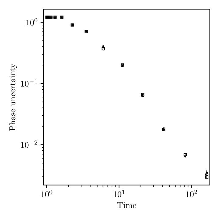
The results of realisations of estimation using the gain rate method with entropy gain, sharpening gain, and the hybrid method are plotted in figure S.2. For times shorter than twice the SPAM time the phase uncertainty decreases little because we can only perform one measurement. For times slightly more than twice the SPAM time the situation is similar to the case discussed in the main text since applying large values of does not significantly impact the experiment time unless . In the large limit we approach the usual situation in quantum metrology , however since in this case is limited by decoherence we never reach this limit. All three of the plotted methods preform similarly. Initially this is consistent with the results of figure 5 for short times. In the large limit the situation becomes similar to the situation in figure 6 for longer times, where all three methods perform similarly when decoherence is included in the model of the estimator. Thus, we see that the results in the limiting cases of the relation between and provide an indication of each method’s performance in the intermediate case.
S.III Multi-step gain method
Supposing we have a prior probability density at step of a sequence of measurements, we calculate the maximum expected knowledge (sharpness or entropy) gain for step as for a single measurement using (7) or (9) for the sharpness or entropy gain, respectively. We calculate the maximum expected gain for two measurements as
Since depends on , it implicitly depends on the outcome . Therefore we write , to denote the values optimised conditioned on a particular measurement outcome at step . We can similarly calculate the maximum expected gain for three measurements as
where the subscript in is to remind us that this quantity depends on the measurement outcome at step . Applying this recursively we can write the maximum expected gain for measurements as
| (S.1) |
Since the number of possible outcomes for the next measurements is , the computation of the multi-step gain generally grows exponentially with the number of measurements. For this reason algorithms S.1 and S.2 are written to compare measurement sequences of approximately equal time that contain at most 5 measurements. In general the gain calculations (7), (9) don’t require all coefficients in (2) allowing a more efficient computation of the multi-step gain.
To understand the effective functions maximised by the multi-step method (in the noise-free case), we calculate the multi-shot gains for sequences with approximately equal time as detailed in algorithm S.2. We assume the usual experiment times in sequential metrology experiments, i.e. , and perform estimation using a total time of starting from a uniform prior. In figure S.3 we then plot the cumulative difference in expected gain for the next measurement between consecutive -values:
| (S.2) |
where the values of are determined as in algorithm S.2. The gain difference calculated in (S.2) is adjusted between intervals with multiple -values by comparing the first -value of consecutive intervals (as in algorithm S.4). The values plotted for are set to zero. In this way the plotted values show an effective function that is maximised (locally) by algorithm S.5.
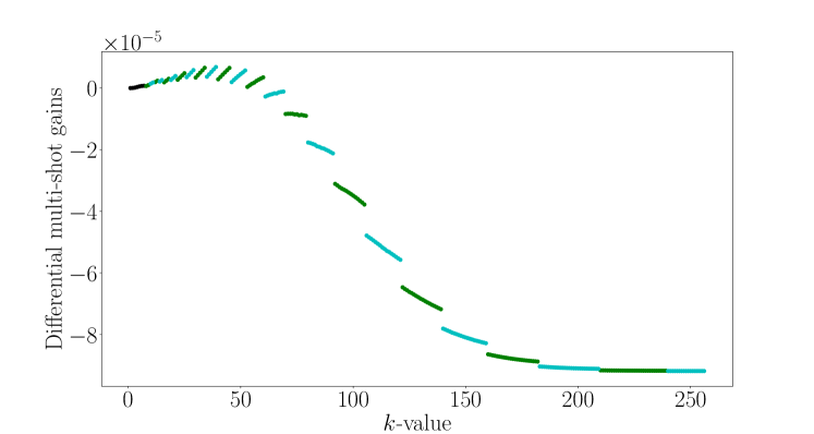
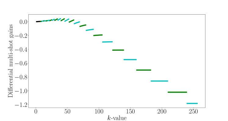
We see that the differential gains for both expected sharpness and entropy gains show a global maximum around . However the differences in multi-shot gains oscillate due to the fact that the times of the multi-step sequences are only approximately equal. Due to these oscillations, algorithm S.4 tends to stop at a local maximum. In algorithm S.5 we always start the search at so that the value of returned is typically much lower than the optimal value suggested by the plotted differential gains. Using the gain rate method to determine the choice of for this measurement gives to maximise the expected sharpness (entropy) gain rate. More efficient methods to find the global maximum of the plotted functions could potentially also lead to accurate estimation procedures.
S.IV Computational complexity of contractions
In this section we derive an upper bound on the number of coefficients needed for the Fourier series when using the contraction method, under the assumption that is Gaussian. In particular, since is periodic, we assume that it would have the form
where is the mean phase, and the Holevo variance is . We have written the sum to here; below we will consider the number of coefficients that would be used in an estimation sequence.
In the following we analyse the case where we perform contractions with , so that after performing contractions we go from a representation on an interval of size to a representation on an interval of size . Since is a measure for the probability of the system phase we are trying to estimate, we will quantify the probability of the system phase being outside the interval represented by after a single contraction by
where in the second line we have used the fact that the result is independent of the mean phase so that we can, without loss of generality, set to zero. The last line follows from solving the integral and relabelling the index of the sum to include only the odd values of in the third line (the integral is zero for even values of ). Although we have not found a solution to the infinite series, we find that is very close to the corresponding quantity for a non-periodic Gaussian,
when is less than .
If we specify an upper bound on the desired probability that the system phase cannot be represented after performing a contraction, then we obtain an upper bound on the standard deviation, , before we should perform a contraction:
| (S.3) |
where is the inverse complementary error function. As mentioned in the main text, we expect from Fourier analysis that the number of coefficients is inversely proportional to (and therefore to ). We can see this in the case of a Gaussian by assuming that any numerical representation will have a finite machine precision. Let be the smallest value that can be represented numerically. Then for the highest order coefficient that can be represented, we have , so
| (S.4) |
Substituting (S.3) into (S.4), we obtain a relation between the probability of an error, , and the number of coefficients:
| (S.5) |
If we now have a that is Gaussian with standard deviation given by (S.3) and that requires a representation to machine precision using coefficients, as given by (S.5), then the probability of an error after performing one contraction with will be less than . At this point we would have a density requiring only coefficients and we could continue estimation until the standard deviation of would be , and that of represented by this contraction would be . Now would have coefficients and we would need to perform another contraction to avoid increasing above . If we would perform a second contraction the total probability that either the first or the second contraction would lead to an error would be . To keep the total error probability below the original value of we would then want to use slightly more coefficients to begin with so that is twice as small.
More generally, if we perform a total of contractions, the total error probability is less than , and from (S.5) we should use a number of coefficients
A representation without contractions would require coefficients. Let be the number of coefficients required to keep the error probability below for a single contraction:
We have , so , and we can write an upper bound on the number of coefficients when using contractions as a function of the number of coefficients that would be needed without using contractions:
| (S.6) |
In figure S.4 we plot the upper bound (S.6) with and . We see that it scales slower than suggesting that the we can use a number of coefficients while keeping the total probability that an error occurs below .
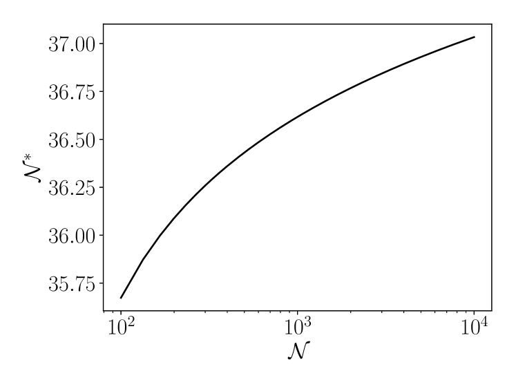
To determine the asymptotic complexity of in terms of we make use of an asymptotic expansion of , for [92, 93]:
| (S.7) |
where
As , and , but each term in (S.7) will be . Since
as . Then to go further, as , we have . From this result we have .
We note that the bound (S.6) is only of practical interest for determining what value of should be reached before performing a contraction with a certain error probability, if is Gaussian. Since we have not shown this in any of the estimation methods we have studied in the main text it cannot be used there. In those cases the value of to be reached before contracting is determined empirically from simulation. But the purpose of the bound (S.6) is mainly to determine what potential the method of using contractions has to reduce computational complexity, rather than to be a practical way of calculating the required value of .
S.V Expected entropy gain
In this section we show the relation between the expected entropy gain (8) and the Kullback-Leibler divergence (KL divergence), and we derive equation (9). Starting from the definition of the expected entropy gain (8), we can rewrite the entropy of the posterior (we sometimes write for short)
where is the KL divergence of the posterior from the prior, and is the cross entropy. Noting that
we see that
i.e. the expected entropy gain is equal to the expected KL divergence. We can rewrite this as
We would like to rewrite the first term with the integral in a form that can be computed more efficiently.
S.V.1 Solving the integral
We have
Let , . Then we have
We can work out the terms in the last line using the Taylor series form of 101010This is possible since .:
So we have
Using this result, we have
and
so
We can rewrite the integral term
so
| (S.8) |
That solves the integral, but we are left with some infinite series that are not very practical for computation. Ideally we would like to have an expression that is a sum over the coefficients of the prior, but without any other infinite series.
S.V.2 Simplifying and solving the series
Using some results from [95], we find the following series solutions
| (S.9) |
| (S.10) |
| (S.11) |
| (S.12) |
which will be used in the derivation below.
We rewrite the sum over in (S.8) separately for the cases where is even or odd. If is even, we have
For every term in the sum with a positive value of there is another term with the same value of , but negative; and there is one term with . So we can rewrite the sum as
We can use the property of binomial coefficients:
Also noting that 111111This is required by normalisation of . we can rewrite the sum as
Similarly, if is odd, we can write
Now let
to simplify the notation. So splitting the sum over into even and odd parts, we have
Now we consider the even part of the sum:
For the odd part we have
So if we combine everything we have
| (S.13) |
There are now four terms in the infinite sum over . The first is
| (S.14) |
The second is
Using the solution to the infinite series:
| (S.15) |
we can rewrite the second term as
Using the result (S.9) we find this is equal to
| (S.16) |
where we defined
| (S.17) |
Next we consider the third term in the infinite sum in (S.13):
The last series over is given by (S.15) (within a factor of two), so we have
Using (S.10) we find this is equal to
| (S.18) |
where we defined
| (S.19) |
Last we consider the fourth term in the infinite sum in (S.13):
Here the last series over is given by (for ; we will need to consider the case separately)
and for
so we have (for )
Using (S.11) we find this is equal to
| (S.20) |
where we defined
| (S.21) |
Finally, for the case in the fourth term in (S.13), we have
Using (S.12) we can rewrite this as
| (S.22) |
where we defined
| (S.23) |
S.V.3 Summary
S.V.4 Limiting cases
If , then , and we have
and , so
If we also have , then , and we have
If , then and we have
Since in this case , this is
as expected, since no information about is given by the measurement.
Finally, we consider the case . Then , and we have
and
and since ,
But we see that the value of
is undefined. Recalling that this was the result of the series
we can see that if we set , we have
Similarly, the value of is undefined. We see that all terms in are zero, except one, which becomes undefined at ; this is the term that results from the series:
But since the series term diverges, we need to take the limit:
So . Putting these results back together, we have
Similarly to the case, when the measurement gives no information about so the expected entropy gain is zero.
S.VI Expected sharpness gain
The sharpness at step is
We define the expected sharpness gain for step :
We have
| (S.25) |
Using (S.25), we have
| (S.26) |
S.VI.1 Limiting cases
If
and if
as expected. And if
as expected.