Time Discretization From Noncommutativity

In general relativity spacetime itself is dynamical, therefore any theory of quantum gravity will imply a quantum spacetime. There are different ways to implement this quantization, and one of the most popular ones is to mimic what has been done for ordinary quantum mechanics, and consider that the algebra generated by the coordinate functions become noncommutative, thus defining a noncommutative geometry. Different flavours of noncommutative spaces based on noncommuting coordinates have appeared. The most promising of those have a deformed symmetry, described by a quantum group, or a Hopf algebra.

We will work in a particular kind of noncommutative spacetime in four dimensions, based on the following commutation relations among the coordinate functions:

	$\displaystyle[x^{0},x^{i}]$	$\displaystyle=$	$\displaystyle\mathrm{i}\lambda{\epsilon^{i}}_{j3}x^{j}$
	$\displaystyle{[}x^{i},x^{j}{]}$	$\displaystyle=$	$\displaystyle 0$		(1)

where $\lambda$ is a constant with the dimensions of length and all other commutators among the coordinate functions vanish. Notice that the third coordinate $x^{3}$ is central, i.e. it commutes with all other coordinates. This form of noncommutativity is a particular kind of Lie algebra type noncommutativity, the underlying Lie algebra being the Euclidean algebra, which goes back to at least [1] (also see [2]). In the context of twisted symmetries it was discussed by Lukierski and Woronowicz in [3]. In [4] it was christened $\rho$-Minkowski because what we call $\lambda$ is called $\rho$ in that paper. We changed the notation to reserve the use of $\rho$ for the radius in cylindrical coordinates. In that paper it was shown that the principle of relative locality [5] holds. This kind of noncommutativity might have concrete physical interest [6, 7] and even phenomenological/observational consequences [8]. A field theory of this space has been constructed in [9].

Commutation relations similar to the ones considered here, and in the above references, have appeared in the definition of the “noncommutative cylinder” [10, 11, 12, 13, 14, 15]. This is an example of a two-dimensional space with a compact dimension, with a commutation relation similar to (1) (or rather (6) below). In particular in [11] time discretization, one of the results of this paper, was noted. Our discussion is however in four dimensions, there are no compact dimensions and the symmetries of the space are recovered in a quantum manner.

Emergence of a discrete time, which is one of the main points of this paper is fascinating. Its origin goes back to no less than C.N. Yang in 1947 [16], or even earlier to Levi [17] who coined the term “Chronon”. Discrete time also appeared in 2+1 gravity thanks to the work of ’t Hooft [18] (see also [19]). The point of view presented here is however novel, in that it connects to deformed symmetries and a promising quantum space.

We study the kinematics of this noncommutative space using the tools developed for usual quantum mechanics, namely quantise the space associating to it an algebra of operators, obtain a concrete representation of them on some Hilbert space, whose vectors are pure states, diagonalise sets of completely commuting observables and use the known measurement theory, namely that the possible results of a measurement are given by the eigenvalues of the observables with probabilities given by the spectral decomposition of self-adjoint operators. The word “quantum” in this context is ambiguous, we use it in the sense that our space is described by operators. But Planck’s action constant $\hbar$ plays no role. We are at a purely kinematical level. Incidentally, this will allow us to freely talk of “time operator”, an object which in usual quantum mechanics is problematic. For a recent point of view see [20] and references therein. If we identify $\lambda$ with Planck’s length, then we are in a situation in which the inverse of the speed of light $c$ and the gravitational constant cannot be ignored, but the quantum of action can.

This kind of analysis was performed for the better known $\kappa$-Minkowski spacetime in [21, 22, 23]. The commutation relations in that case are of the kind

$$[x^{0},x^{i}]=\frac{\mathrm{i}}{\kappa}x^{i}\ ;\ [x^{i},x^{j}]=0$$

(2)

It was found that only states localised at the origin, identified with the position of a local observer, can be absolutely localised. States at a distance cannot be precisely localised. This is a consequence of an uncertainty principle which reads as

$$\Delta x^{0}\Delta x^{i}\geq\frac{1}{2\kappa}\left|\langle x^{i}\rangle\right|.$$

(3)

Let us analyse the case of $\rho$-Minkowski. The relations (1) are clearly of an angular nature. For this reason we work in cylindrical coordinates defined as

$$\rho=\sqrt{{x^{1}}^{2}+{x^{2}}^{2}}\ ,\ z=\ x^{3}\ ,\ t=\frac{x^{0}}{c}\ ,\ \varphi=\arctan\frac{x^{2}}{x^{1}}$$

(4)

One could be tempted to say that in these coordinates the only nonzero commutator is

$$[t,\varphi]=\mathrm{i}\lambda$$

(5)

but this expression clearly does not make sense. The quantity $\varphi$ is not a single valued function and upon quantisation no self-adjoint operator would correspond to it. A correct expression is

$$[t,{\mathrm{e}}^{\mathrm{i}\varphi}]=-\mathrm{i}\lambda{\mathrm{e}}^{\mathrm{i}\varphi}$$

(6)

where ${\mathrm{e}}^{\mathrm{i}\varphi}$ is a legitimate well defined unitary operator.

As we said, we want to borrow the analysis from the usual quantum mechanics of point particles in three dimensions, for example. In this case we have various standard sets of mutually commuting operators. For example we can consider the three position coordinates $q^{i}$, and represent them as multiplicative operators on functions belonging to $L^{2}(\mathbb{R}^{3})$, i.e. functions on configuration space. Alternatively we could consider $p_{i}$ as complete sets, and consider functions in Fourier transform, and position acting as a differential operator. In both these cases the spectrum is continuous (the whole line for each component), and the eigenstates are improper vectors (distributions), Dirac $\delta$’s and plane waves respectively. Other standard choices are the three number operators

$$N_{i}=\frac{1}{2}(p_{i}^{2}+q_{i}^{2})-\frac{1}{2}$$

(7)

In this case the spectrum is discrete and the eigenfunctions are represented by Hermite polynomials multiplied by a Gaussian. All sort of combinations of continuous and discrete spectrum can occur; for example, for the hydrogen atom a complete set of observables is represented by the Hamiltonian itself, the square of the angular momentum and one of its components. In this case the spectrum has continuous and discrete components, and the eigenfunctions are combinations of Laguerre polynomials, exponential functions and spherical harmonics. Any complete set will do, as long as the operators belonging to the set are self-adjoint and commute.

An important aspect to note is that the quantization of phase space has representations on square integrable functions of a lower dimensional space. The choice of the complete set indicates which observables we may simultaneously measure. Let us consider first the case of $L^{2}(\mathbb{R}^{3})$ functions and configuration space variables as a complete set of commuting observables. Classically the momentum of a particle is related to the velocity, proportional to it in the absence of magnetic forces. There is no problem in the perfect localisation in position and momentum. The $\delta$’s are states of the commutative algebra of position and momentum variables. Quantum mechanically it is still possible to localise the state in position space, but to do this it is necessary to superimpose particles of all momenta:

$$\delta(\vec{x})=\frac{1}{2\pi}\int_{-\infty}^{\infty}\!{\mathrm{d}}^{3}k\,{\mathrm{e}}^{\mathrm{i}\vec{k}\cdot\vec{x}}$$

(8)

Good knowledge of position implies bad knowledge of momentum, and viceversa. Both position and momentum are self-adjoint non bounded operators with spectrum the real line. Up to signs and complex conjugations they are symmetrical in the theory. Likewise, to obtain the improper eigenfunction $\delta$ as a superposition of eigenfunctions of the number operators, an infinite series is necessary, whose coefficients are not particularly simple or illuminating. Conversely, to express the eigenfunctions of the number operator in the basis in which position is diagonal we need to give infinite information, i.e. a function of the variables: in this case an Hermite polynomial times a Gaussian. All this is of course well known. We just stress it to compare with the noncommutative cases below.

Let us first review what has been done for $\kappa$-Minkowski space-time in [21, 22, 23]. In this case the only non trivial commutator can be expressed as

$$[t,r]=\frac{\mathrm{i}}{\kappa}r.$$

(9)

A possible set of commuting coordinates is thus given by the spatial coordinates¹¹1We have already commented on the fact that $\varphi$, an $\lambda$ are not selfadjoint operators, we nevertheless use notations like $\{r,\lambda,\varphi\}$ as an useful shorthand. What we mean is that the observables are the $\{x^{i}\}$’s acting on functions written in spherical (and later cylindrical) coordinates., and it is possible to represent $t$ as an operator acting on functions of $r$ as a dilation:

$$t=\frac{\mathrm{i}}{\kappa}\left(r\partial_{r}+\frac{3}{2}\right)$$

(10)

where the $\frac{3}{2}$ factor is necessary for self-adjointness. The time operator has a continuous spectrum, and the (improper) eigenfunctions are the distributions

$$T_{\tau}=\frac{r^{-\frac{3}{2}-\mathrm{i}\tau}}{\kappa^{\mathrm{i}\tau}}=r^{-\frac{3}{2}}{\mathrm{e}}^{-\mathrm{i}\tau\log\left(r\kappa\right)}$$

(11)

which play the same role as plane waves in quantum mechanics for the operator $p$. The expansion of functions in the basis of the $\tau$ operator is therefore provided by monomials, suggesting the use of the Mellin transform, which replaces the Fourier transform. Hence, a state shall be written either as a function of $r\kappa$, or of $\tau={x^{0}}\kappa$, according to:

	$\displaystyle\psi(r,\theta,\varphi)$	$\displaystyle=$	$\displaystyle\frac{1}{\sqrt{2\pi}}\int_{-\infty}^{\infty}{\mathrm{d}}\tau\,r^{-\frac{3}{2}}{\mathrm{e}}^{-\mathrm{i}\tau\log\left(r\kappa\right)}\widetilde{\psi}(\tau,\theta,\varphi),$
	$\displaystyle\widetilde{\psi}(\tau,\theta,\varphi)$	$\displaystyle=$	$\displaystyle\frac{1}{\sqrt{2\pi}}\int_{0}^{\infty}r^{2}{\mathrm{d}}r\,r^{-\frac{3}{2}}{\mathrm{e}}^{\mathrm{i}\tau\log\left(r\kappa\right)}\psi(r,\theta,\varphi).$		(12)

The transformation is an isometry of $L^{2}$, and $|\psi|^{2}$ and $|\widetilde{\psi}|^{2}$ are the probability densities to find the particle at position $r$ or time $\tau$ respectively.

The uncertainty relation (3) means that it is impossible to localise exactly a state both temporally and radially, except when the space is localised at $r=0$. The origin is the point at which the observer is located, and is not a “special point”. Another observer will be located at its own (different) origin, and will be able to localize states near to him.

As for space-time symmetries, let us recall that $\kappa$-Minkowski commutation relations are not Poincaré invariant; indeed they are $\kappa$-Poincaré invariant, and translations in this case are not commuting. Therefore there is no contradiction in the fact that it is impossible for Alice to locate a state which Bob may. Alice cannot even precisely locate Bob! To summarise, for $\kappa$-Minkowski space-time we have two complete sets of operators, $\{x^{i}\}=\{r,\theta,\varphi\}$, $\{t,\theta,\varphi\}$, and the two variables $t$ and $r$ are connected by a Mellin rather than a Fourier transform. The noncommuting operators do not appear symmetrically. They are both unbounded with continuous spectrum, but while the spectrum of $r$ is the positive real line, that of $t$ is the whole of $\mathbb{R}$. The eigenstates of the two are related by Mellin, anti-Mellin transforms, which are not symmetric as in the Fourier case. The final result is that states along the time axis can be localised, while states at a distance from the origin need to superimpose states of arbitrary time. We refer to [21, 22, 23] for details.

For the case of $\rho$-Minkowski there are two natural choices of complete sets of commuting observables. On the one side we have again the three position variables, which is convenient to express in cylindrical coordinates $\{\rho,z,\varphi\}$, or we may choose to have time among the observables and have $\{\rho,z,t\}$.

The three position operators act as multiplication operators, with $\rho$ and $z$ selfadjoint, and ${\mathrm{e}}^{\mathrm{i}\varphi}$ unitary. The pure states of this algebra, like the previous cases, are the Dirac $\delta$ functions localised at the points of $\mathbb{R}^{3}$. It is possible to completely localise a state at any point. The time operator acts as the angular momentum in the $z$ direction. This leads to the central observation of this note:

The relation between the two bases is given by the Fourier series expansion of the angular part:

$$\psi(\rho,z,\varphi)=\sum_{n=-\infty}^{\infty}\psi_{n}(\rho,z){\mathrm{e}}^{\mathrm{i}n\varphi}$$

(13)

The time and angular variable are dual, but since $\varphi$ is not a good self-adjoint operator we cannot write the equivalent of Heisenberg uncertainty as $\Delta t\Delta\varphi$. Nevertheless a similar reasoning can be made. As is known an eigenstate of the angular variable would need

$$\delta(\varphi)=\frac{1}{2\pi}\sum_{n=-\infty}^{\infty}{\mathrm{e}}^{\mathrm{i}n\varphi}.$$

(14)

On the other side, after a time measurement, which has given as result $n_{0}\lambda$, the system will be in an eigenstate of the time variable, namely a single ${\mathrm{e}}^{\mathrm{i}n_{0}\varphi}$. This means that an absolutely precise measurement of time would return a state which is uniformly dense in the angular variable. If one measures instead time with some uncertainty, i.e. uses a certain number of Fourier modes to build a state peaked around some time, then the corresponding uncertainty in the angular variable is given by the fact that only a finite set of elements of the basis is available. If one identifies the length $\lambda$ with Planck length, converting this quantity in time units by means of the speed of light gives for the quantum of time a quantity of the order of $5.39\ 10^{-44}\,$sec. The most accurate measurement of time available to date is of the order of $10^{-19}\,$sec. [24] Let us make a very heuristic order of magnitude argument. We may say that such a measurement needs the superposition of something like $10^{25}$ quanta of time. In order to localise with absolute precision the angular component of a state all infinite Fourier modes are needed, but a delta function can be well approximated by the Dirichlet nucleus

$$\delta_{N}=\sum_{n=-N}^{N}{\mathrm{e}}^{\mathrm{i}n\varphi}=\frac{1}{2\pi}\frac{\sin(N+\frac{1}{2})\varphi}{\sin\frac{N}{2}\varphi}.$$

(15)

In Fig. 1 we plot $\delta_{N}$ for three (extremely small!) values of $N=5,10,15$.

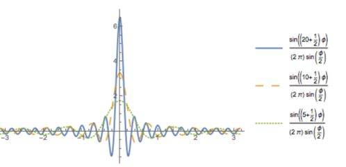
This means that the most precise experiment is using $N\sim 10^{25}$. In this case the first zero of the Dirichlet nucleus (the width of the main peak of the function) is for $\varphi\sim 10^{-25}$. We may assume this to be the uncertainty in an angle determination. To translate this as an uncertainty in position we need an estimate of the radius $\rho$, the larger $\rho$, the larger the uncertainty. The uncertainty at the edge of the observable universe ($10^{26}\,$m) is of the order of meters. An uncertainty on the localisation of objects we can live with!

An important aspect of $\rho$-Minkowski space-time is that, like $\kappa$-Minkowski [25, 26, 27], it may be regarded as the homogeneous space of a quantum group (i.e.  a quantum Hopf algebra) [28]. Therefore, although its commutation relations violate standard Poincaré symmetry, they are covariant under the action of the appropriate deformation of the Poincaré group. The latter may be described following two approaches, which are dual to each other: the Lie algebra deformation with its universal enveloping algebra and the group algebra deformation, namely the deformation of the algebra of functions on the group. They both yield to quantum Hopf algebras, dually related, which are both referred to as the quantum group $\mathcal{G}_{q}$, with $\mathcal{G}$ the starting Lie group, and $q$ the deformation parameter. For the case at hand the former approach has been described in [29], and further analysed in [9] in the context of field theory, whereas the latter has not been investigated up to now, to our knowledge. Interestingly, the two points of view may be related to observer-dependent and particle dependent transformations. Let us see how it works in the present context.

The noncommutative algebra (1) may be realised on the algebra of functions on $\mathbb{R}^{4}$ in terms of a star product associated with a twist operator which reads

	$\displaystyle\mathcal{F}$	$\displaystyle=$	$\displaystyle\exp{\left\{-\frac{\mathrm{i}\lambda}{2}\left[\partial_{0}\otimes\left(x^{2}\partial_{1}-x^{1}\partial_{2}\right)-\left(x^{2}\partial_{1}-x^{1}\partial_{2}\right)\otimes\partial_{0}\right]\right\}}$		(16)
		$\displaystyle=$	$\displaystyle\exp{\left\{\frac{\mathrm{i}\lambda}{2}\left(\partial_{0}\otimes\partial_{\varphi}-\partial_{\varphi}\otimes\partial_{0}\right)\right\}}.$

The star-product is therefore defined according to

$$(f\star g)(x):=\mu_{\star}(f\otimes g)(x)=\mu_{0}\circ\mathcal{F}^{-1}(f\otimes g)(x).$$

(17)

Since the algebra is noncommutative, so is the combination of plane waves, and the sum rule of momenta:

$${\mathrm{e}}^{-\mathrm{i}p\cdot x}\star{\mathrm{e}}^{-\mathrm{i}q\cdot x}={\mathrm{e}}^{-\mathrm{i}(R_{i}^{j}(p_{j}+q_{j})x^{i}},$$

(18)

with $R$ the following matrix:

$$R(t)\equiv\left(\begin{array}[]{cccc}\cos{\left(\frac{\lambda t}{2}\right)}&0&0&\sin{\left(\frac{\lambda t}{2}\right)}\\ 0&1&0&0\\ 0&0&1&0\\ -\sin{\left(\frac{\lambda t}{2}\right)}&0&0&\cos{\left(\frac{\lambda t}{2}\right)}\end{array}\right).$$

(19)

In the twist approach, the Poincaré generators act undeformed on a single copy of the algebra of observables, with standard Lie brackets; but, in order to act on products of observables (and therefore on the commutator (1)), the coproduct of Lie algebra generators has to be twisted for the consistency of the whole enveloping algebra $\mathcal{U}(\mathfrak{p})$, according to $\Delta_{\mathcal{F}}=\mathcal{F}\Delta\mathcal{F}^{-1}$. This entails a twisted Leibniz rule, so that for $X\in\mathfrak{p}$

$$X\triangleright f\star g:=\mu_{\star}\circ\Delta_{\mathcal{F}}(X)(f\otimes g)$$

(20)

The twisted coproduct of Poincaré generators [29] is given by:

	$\displaystyle\Delta^{\cal F}P_{0}=P_{0}\otimes 1+1\otimes P_{0},$
	$\displaystyle\Delta^{\cal F}P_{3}=P_{3}\otimes 1+1\otimes P_{3},$
	$\displaystyle\Delta^{\cal F}P_{1}=P_{1}\otimes\cos\left(\frac{\lambda}{2}P_{0}\right)+\cos\left(\frac{\lambda}{2}P_{0}\right)\otimes P_{1}+P_{2}\otimes\sin\left(\frac{\lambda}{2}P_{0}\right)-\sin\left(\frac{\lambda}{2}P_{0}\right)\otimes P_{2},$
	$\displaystyle\Delta^{\cal F}P_{2}=P_{2}\otimes\cos\left(\frac{\lambda}{2}P_{0}\right)+\cos\left(\frac{\lambda}{2}P_{0}\right)\otimes P_{2}-P_{1}\otimes\sin\left(\frac{\lambda}{2}P_{0}\right)+\sin\left(\frac{\lambda}{2}P_{0}\right)\otimes P_{1},$		(21)

while the twisted coproduct of Lorentz generators is:

	$\displaystyle\Delta^{\cal F}M_{31}=M_{31}\otimes\cos\left(\frac{\lambda}{2}P_{0}\right)+\cos\left(\frac{\lambda}{2}P_{0}\right)\otimes M_{31}+M_{32}\otimes\sin\left(\frac{\lambda}{2}P_{0}\right)-\sin\left(\frac{\lambda}{2}P_{0}\right)\otimes M_{32}$
	$\displaystyle\hskip 42.67912pt-P_{1}\otimes\frac{\lambda}{2}M_{12}\cos\left(\frac{\lambda}{2}P_{0}\right)+\frac{\lambda}{2}M_{12}\cos\left(\frac{\lambda}{2}P_{0}\right)\otimes P_{1}$
	$\displaystyle\hskip 42.67912pt-P_{2}\otimes\frac{\lambda}{2}M_{12}\sin\left(\frac{\lambda}{2}P_{0}\right)-\frac{\lambda}{2}M_{12}\sin\left(\frac{\lambda}{2}P_{0}\right)\otimes P_{2},$
	$\displaystyle\Delta^{\cal F}M_{32}=M_{32}\otimes\cos\left(\frac{\lambda}{2}P_{0}\right)+\cos\left(\frac{\lambda}{2}P_{0}\right)\otimes M_{32}-M_{31}\otimes\sin\left(\frac{\lambda}{2}P_{0}\right)+\sin\left(\frac{\lambda}{2}P_{0}\right)\otimes M_{31}$
	$\displaystyle\hskip 42.67912pt-P_{2}\otimes\frac{\lambda}{2}M_{12}\cos\left(\frac{\lambda}{2}P_{0}\right)+\frac{\lambda}{2}M_{12}\cos\left(\frac{\lambda}{2}P_{0}\right)\otimes P_{2}$
	$\displaystyle\hskip 42.67912pt+P_{1}\otimes\frac{\lambda}{2}M_{12}\sin\left(\frac{\lambda}{2}P_{0}\right)+\frac{\lambda}{2}M_{12}\sin\left(\frac{\lambda}{2}P_{0}\right)\otimes P_{1},$
	$\displaystyle\Delta^{\cal F}M_{30}=M_{30}\otimes 1+1\otimes M_{30}-\frac{\lambda}{2}P_{3}\otimes M_{12}+\frac{\lambda}{2}M_{12}\otimes P_{3},$
	$\displaystyle\Delta^{\cal F}M_{12}=M_{12}\otimes 1+1\otimes M_{12},$
	$\displaystyle\Delta^{\cal F}M_{10}=M_{10}\otimes\cos\left(\frac{\lambda}{2}P_{0}\right)+\cos\left(\frac{\lambda}{2}P_{0}\right)\otimes M_{10}+M_{20}\otimes\sin\left(\frac{\lambda}{2}P_{0}\right)-\sin\left(\frac{\lambda}{2}P_{0}\right)\otimes M_{20}$
	$\displaystyle\Delta^{\cal F}M_{20}=M_{20}\otimes\cos\left(\frac{\lambda}{2}P_{0}\right)+\cos\left(\frac{\lambda}{2}P_{0}\right)\otimes M_{20}-M_{10}\otimes\sin\left(\frac{\lambda}{2}P_{0}\right)+\sin\left(\frac{\lambda}{2}P_{0}\right)\otimes M_{10}.$		(22)

The universal enveloping algebra of $\mathfrak{p}$, endowed with the twisted coproduct above, an antipode and a co-unit, may be shown to yield a quantum Hopf algebra, or equivalently, a quantum group, which we shall refer to as the $\rho$-Poincaré quantum group $U_{\rho}({\mathfrak{p}})$ (remember that the deformation parameter is $\lambda$ in our case, but we keep the notation $\rho$ to adhere to the existing literature). For the purposes of the paper we don’t need to enter the technical details of the construction. What is relevant to us is that the commutation relations (1) are twist-covariant, namely covariant under the action of the Poincaré generators if their action is implemented through the appropriate co-product

$$X\triangleright[f,g]_{*}:=\mu_{\star}\circ\Delta_{\mathcal{F}}(X)(f\otimes g-g\otimes f).$$

(23)

Infinitesimal transformations of the observables, realised through the action of the deformed Hopf algebra $U_{\lambda}({\mathfrak{p}})$ are usually considered when dealing with active transformations of physical quantities in a fixed reference frame.

Let us now consider finite transformations, which are especially relevant in connection with passive, or observer transformations [30, 31]. The deformation of the co-product in the Lie algebra of the group has its counterpart in the deformation of the product in the algebra of functions on the group manifold. In particular, it will affect the parameters of the Poincaré group, $(\Lambda^{\mu}_{\nu},a^{\mu})\in\mathcal{F}({\mathcal{P}})$. Following [32] (see also [33]) we first construct the Poisson-Lie bracket for $\mathcal{F}({\mathcal{P}})$ and then obtain the quantum group ${\mathcal{P}}_{\lambda}$ by replacing the PL-bracket with the commutator. To this, we read off the $r$-matrix from the twist operator (16), it being $\mathcal{F}=1+\frac{1}{2}r+\dots$,

$$r=-\mathrm{i}\lambda(P_{0}\wedge M_{12})\in\mathfrak{p}\otimes\mathfrak{p}$$

(24)

which satisfies the classical Yang-Baxter equation [32]. In terms of $r$ we define the Poisson-Lie bracket on the group manifold

$$\{f,h\}=\lambda\left(X_{0}^{R}\wedge X^{R}_{12}-X_{0}^{L}\wedge X^{L}_{12}\right)(df,dg)\;\;f,g\in\mathcal{F}(\mathcal{P})$$

(25)

with $X_{0}^{R,L},X^{R,L}_{12}$ the right and left invariant vector fields corresponding to the Lie algebra generators $P_{0},M_{12}$. They read

$\begin{aligned} X_{\alpha}^{L}&=\Lambda^{\sigma}_{\alpha}\frac{\partial}{\partial a^{\sigma}},\;\;\;&X_{\alpha\beta}^{L}&=\Lambda^{\sigma}_{\alpha}\frac{\partial}{\partial\Lambda^{\sigma\beta}}-\Lambda^{\sigma}_{\beta}\frac{\partial}{\partial\Lambda^{\sigma\alpha}}\\ X_{\alpha}^{R}&=\frac{\partial}{\partial a^{\alpha}},\;\;\;&X_{\alpha\beta}^{R}&=\Lambda_{\beta\sigma}\frac{\partial}{\partial\Lambda^{\alpha}_{\sigma}}-\Lambda_{\alpha\sigma}\frac{\partial}{\partial\Lambda^{\beta}_{\sigma}}+a_{\beta}\frac{\partial}{\partial a_{\alpha}}\end{aligned}$

(26)

and we compute

	$\displaystyle\{{\Lambda^{\mu}}_{\nu},{\Lambda^{\rho}}_{\sigma}\}$	$\displaystyle=$	$\displaystyle 0$		(27)
	$\displaystyle\{{\Lambda^{\mu}}_{\nu},a^{\rho}\}$	$\displaystyle=$	$\displaystyle\lambda\big{[}-\delta^{\rho}_{0}(\Lambda_{2\nu}\delta^{\mu}_{1}-\Lambda_{1\nu}\delta^{\mu}_{2})+{\Lambda^{\rho}}_{0}({\Lambda^{\mu}}_{1}\eta_{2\nu}-{\Lambda^{\mu}}_{2}\eta_{1\nu})\big{]}$		(28)
	$\displaystyle\{a^{\mu},a^{\nu}\}$	$\displaystyle=$	$\displaystyle\lambda\big{[}\delta^{\mu}_{0}(a_{2}\delta^{\nu}_{1}-a_{1}\delta^{\nu}_{2})-{\delta^{\nu}}_{0}(a_{2}\delta^{\mu}_{1}-a_{1}\delta^{\mu}_{2})\big{]}.$		(29)

We thus perform the standard quantization by replacing Poisson brackets with $-\mathrm{i}$ times the commutators. We obtain

	$\displaystyle[{\Lambda^{\mu}}_{\nu},{\Lambda^{\rho}}_{\sigma}]$	$\displaystyle=$	$\displaystyle 0$		(30)
	$\displaystyle{[}{\Lambda^{\mu}}_{\nu},a^{\rho}{]}$	$\displaystyle=$	$\displaystyle\mathrm{i}\lambda\big{[}-\delta^{\rho}_{0}(\Lambda_{2\nu}\delta^{\mu}_{1}-\Lambda_{1\nu}\delta^{\mu}_{2})+{\Lambda^{\rho}}_{0}({\Lambda^{\mu}}_{1}\eta_{2\nu}-{\Lambda^{\mu}}_{2}\eta_{1\nu})\big{]}$		(31)
	$\displaystyle{[}a^{\mu},a^{\nu}{]}$	$\displaystyle=$	$\displaystyle\mathrm{i}\lambda\big{[}\delta^{\mu}_{0}(a_{2}\delta^{\nu}_{1}-a_{1}\delta^{\nu}_{2})-\delta^{\nu}_{0}(a_{2}\delta^{\mu}_{1}-a_{1}\delta^{\mu}_{2})\big{]}.$		(32)

Since the composition law of group elements is compatible with Poisson brackets, the coproduct, antipode and counit are undeformed. The algebra $\mathcal{F}_{\lambda}(\mathcal{P})$ with the structures here introduced is a quantum Hopf algebra, the quantum Poincaré group $\mathcal{P}_{\lambda}$ in the dual picture announced before. Not surprisingly, the commutator of translation parameters (32) reproduces the $\rho$-Minkowski algebra (1), the latter being identified with the homogeneous space of the quantum Poincaré group with respect to the undeformed Lorentz subgroup. In other words, the $\rho$-Minkowski space-time is co-acted upon according to

$${x^{\prime}}^{\mu}={\Lambda^{\mu}}_{\nu}\otimes x^{\nu}+a^{\mu}\otimes 1$$

(33)

and commutation relations (1) are covariant under (33), provided (27)-(32) hold.

This completes the picture which allows for equivalent descriptions of the $\rho$-Poincaré group and its action on the $\rho$-Minkowski space-time.

The group algebra approach is useful to understand the observer-dependent transformations²²2 A similar analysis has been performed in [21] for $\kappa$-Minkowski.. The most relevant consequence is that the transformations relating different reference frames belong to a noncommutative algebra. Hence localisability will be subject to limitations as well. States for the algebra generated by coordinates may be more or less sharply localised. When the algebra is noncommuting, there may not be states of absolute localisation. This happens in our case. As a consequence, different observers will not agree in general on the localizability properties of the same state. We have to specify the observer making the observations, and we have been implicitly considering an observer located at the origin. In order to change observer, a Poincaré transformation is needed. But in our case the symmetry is the quantum $\rho$-Poincaré. Accordingly it will be impossible to locate the position of the transformed observer, since translations do not commute.

Since time (and time slices) are discrete there appears to be a universal clock, whose beats give the allowable instants. This is only partially true. It is known (see for example [34, 35]) that periodic functions are only one of the domains of selfadjointness of the operator $-\mathrm{i}\partial_{\varphi}$. A generic domain in which functions are periodic up to a phase ${\mathrm{e}}^{\mathrm{i}\alpha}$ is equally good. The basis of this domain is given by functions of the kind

$$e_{\alpha}={\mathrm{e}}^{\mathrm{i}(n+\alpha)\varphi}$$

(34)

which, together with the coefficients $\psi_{n}(\rho,z)$ in (13), provide an expansion for the vectors of the Hilbert space. The spectrum of the time operator is given by the set $n+\alpha$. The differences between eigenvalues are unchanged, and the effect is a rigid shift. Of course $\alpha$ is itself periodic of period $2\pi$. This however means that a different choice of selfadjointess domain has been made. Time translations are undeformed, and two time-translated observers will be in different, but equivalent domains. A given observer, nevertheless, can only measure quantized time intervals.

We conclude with some comments. There are several noncommutative spaces with discrete features, reviews and references can be found for example in [36, 37]. Although the main motivation of this note was not to present a phenomenological viable model, nevertheless this model might be developed in a more physical direction. A field theory has been built in [9], and it was shown there that decays may be affected. The $S$-matrix for these processes is discussed in [38]. In [8] it was connected to lensing. We feel that $\rho$-Minkowski can be added to the list of viable noncommutative spaces, and its peculiar properties deserve further investigation in a variety of directions.

References

- [1] S. Gutt, An explicit -product on the cotangent bundle of a Lie group, Lett. Math. Phys. 7 (1983) 249.
- [2] J. M. Gracia-Bondia, F. Lizzi, G. Marmo and P. Vitale, Infinitely many star products to play with, JHEP 04 (2002) 026 [hep-th/0112092].
- [3] J. Lukierski and M. Woronowicz, New Lie-algebraic and quadratic deformations of Minkowski space from twisted Poincaré symmetries, Phys. Lett. B 633 (2006) 116 [hep-th/0508083].
- [4] G. Amelino-Camelia, L. Barcaroli and N. Loret, Modeling transverse relative locality, Int. J. Theor. Phys. 51 (2012) 3359 [1107.3334].
- [5] G. Amelino-Camelia, L. Freidel, J. Kowalski-Glikman and L. Smolin, The principle of relative locality, Phys. Rev. D 84 (2011) 084010 [1101.0931].
- [6] M. Dimitrijević Ćirić, N. Konjik and A. Samsarov, Search for footprints of quantum spacetime in black hole QNM spectrum, 1910.13342.
- [7] M. Dimitrijević Ćirić, N. Konjik and A. Samsarov, Noncommutative scalar field in the nonextremal Reissner-Nordström background: Quasinormal mode spectrum, Phys. Rev. D 101 (2020) 116009 [1904.04053].
- [8] G. Amelino-Camelia, L. Barcaroli, S. Bianco and L. Pensato, Planck-scale dual-curvature lensing and spacetime noncommutativity, Adv. High Energy Phys. 2017 (2017) 6075920 [1708.02429].
- [9] M. Dimitrijevic Ciric, N. Konjik, M. A. Kurkov, F. Lizzi and P. Vitale, Noncommutative field theory from angular twist, Phys. Rev. D 98 (2018) 085011 [1806.06678].
- [10] M. Chaichian, A. Demichev and P. Presnajder, Quantum field theory on noncommutative space-times and the persistence of ultraviolet divergences, Nucl. Phys. B 567 (2000) 360 [hep-th/9812180].
- [11] M. Chaichian, A. Demichev, P. Presnajder and A. Tureanu, Space-time noncommutativity, discreteness of time and unitarity, Eur. Phys. J. C 20 (2001) 767 [hep-th/0007156].
- [12] B. P. Dolan, K. S. Gupta and A. Stern, Noncommutative BTZ black hole and discrete time, Class. Quant. Grav. 24 (2007), 1647 [hep-th/0611233].
- [13] A. P. Balachandran, A. G. Martins and P. Teotonio-Sobrinho, Discrete time evolution and energy nonconservation in noncommutative physics, JHEP 05 (2007) 066 [hep-th/0702076].
- [14] D. Bak and K.-M. Lee, Noncommutative supersymmetric tubes, Phys. Lett. B 509 (2001) 168 [hep-th/0103148].
- [15] H. Steinacker, Split noncommutativity and compactified brane solutions in matrix models, Prog. Theor. Phys. 126 (2011) 613 [1106.6153].
- [16] C. Yang, On quantized space-time, Phys. Rev. 72 (1947) 874.
- [17] R. Lévi, Théorie de l’action universelle et discontinue, J. Phys. Radium 8 (1927) 182.
- [18] G. ’t Hooft, Canonical quantization of gravitating point particles in (2+1)-dimensions, Class. Quant. Grav. 10 (1993) 1653 [gr-qc/9305008].
- [19] A. P. Balachandran and L. Chandar, Discrete time from quantum physics, Nucl. Phys. B 428 (1994) 435 [hep-th/9404193].
- [20] P. Aniello, F. Ciaglia, F. Di Cosmo, G. Marmo and J. Pérez-Pardo, Time, classical and quantum, Annals Phys. 373 (2016) 532 [1605.03534].
- [21] F. Lizzi, M. Manfredonia, F. Mercati and T. Poulain, Localization and Reference Frames in -Minkowski Spacetime, Phys. Rev. D99 (2019) 085003 [1811.08409].
- [22] F. Lizzi, M. Manfredonia and F. Mercati, Localizability in -Minkowski spacetime, Int. J. Geom. Meth. Mod. Phys. 17 (2020) 2040010 [1912.07098].
- [23] F. Lizzi, M. Manfredonia and F. Mercati, The momentum spaces of -Minkowski noncommutative spacetime, Nucl. Phys. B 958 (2020) 115117 [2001.08756].
- [24] S. Grundmann, D. Trabert, K. Fehre, N. Strenger, A. Pier, L. Kaiser et al., Zeptosecond birth time delay in molecular photoionization, Science 2020 (2020) 339 [2010.08298].
- [25] J. Lukierski, A. Nowicki and H. Ruegg, Real forms of complex quantum anti-De Sitter algebra U-q(Sp(4:C)) and their contraction schemes, Phys. Lett. B271 (1991) 321 [hep-th/9108018].
- [26] J. Lukierski, A. Nowicki and H. Ruegg, New quantum Poincaré algebra and k deformed field theory, Phys. Lett. B293 (1992) 344 [hep-th/9108018].
- [27] S. Majid and H. Ruegg, Bicrossproduct structure of kappa Poincaré group and noncommutative geometry, Phys. Lett. B334 (1994) 348 [hep-th/9405107].
- [28] V. G. Drinfel’d, Hopf algebras and the quantum Yang-Baxter equation, Sov. Math. Dokl. 32 (1985) 254.
- [29] M. Dimitrijević Ćirić, N. Konjik and A. Samsarov, Noncommutative scalar quasinormal modes of the Reissner–Nordström black hole, Class. Quant. Grav. 35 (2018) 175005 [1708.04066].
- [30] P. Kosinski, J. Lukierski and P. Maslanka, Local d=4 field theory on –deformed Minkowski space, http://arxiv.org/abs/hep-th/9902037v2.
- [31] P. Kosinski, J. Lukierski and P. Maslanka, –deformed Wigner construction of relativistic wave functions and free fields on -Minkowski space, http://arxiv.org/abs/hep-th/0103127v1.
- [32] A. N. P. Vyjayanthi Chari, A guide to quantum groups. Cambridge University Press, 1994.
- [33] P. Kosinski and P. Maslanka, The Kappa-Weyl group and its algebra, 9512018.
- [34] M. Reed and B. Simon, Methods of Modern Mathematical Physics. 2. Fourier Analysis, Self-adjointness. Academic Press, 1, 1975.
- [35] G. Esposito, G. Marmo, G. Miele and G. Sudarshan, Advanced concepts in quantum mechanics. Cambridge University Press, 10, 2014, 10.1017/CBO9781139875950.
- [36] F. Lizzi and P. Vitale, Matrix Bases for Star Products: a Review, SIGMA 10 (2014) 086 [1403.0808].
- [37] F. D’Andrea, F. Lizzi and P. Martinetti, Spectral geometry with a cut-off: topological and metric aspects, J. Geom. Phys. 82 (2014) 18 [1305.2605].
- [38] O. O. Novikov, -symmetric quantum field theory on the noncommutative spacetime, Mod. Phys. Lett. A 35 (2019) 2050012 [1906.05239].