Time-In-Range Analyses of Functional Data Subject to Missing with Applications to Inpatient Continuous Glucose Monitoring–Time-In-Range Analyses of Functional Data Subject to Missing with Applications to Inpatient Continuous Glucose Monitoring
Time-In-Range Analyses of Functional Data Subject to Missing with Applications to Inpatient Continuous Glucose Monitoring
Abstract
Continuous glucose monitoring (CGM) has been increasingly used in US hospitals for the care of patients with diabetes. Time in range (TIR), which measures the percent of time over a specified time window with glucose values within a target range, has served as a pivotal CGM-metric for assessing glycemic control. However, inpatient CGM is prone to a prevailing issue that a limited length of hospital stay can cause insufficient CGM sampling, leading to a scenario with functional data plagued by complex missingness. Current analyses of inpatient CGM studies, however, ignore this issue and typically compute the TIR as the proportion of available CGM glucose values in range. As shown by simulation studies, this can result in considerably biased estimation and inference, largely owing to the nonstationary nature of inpatient CGM trajectories. In this work, we develop a rigorous statistical framework that confers valid inference on TIR in realistic inpatient CGM settings. Our proposals utilize a novel probabilistic representation of TIR, which enables leveraging the technique of inverse probability weighting and semiparametric survival modeling to obtain unbiased estimators of mean TIR that properly account for incompletely observed CGM trajectories. We establish desirable asymptotic properties of the proposed estimators. Results from our numerical studies demonstrate good finite-sample performance of the proposed method as well as its advantages over existing approaches. The proposed method is generally applicable to other functional data settings similar to CGM.
keywords:
Continuous glucose monitoring (CGM); Functional data; Missing data; Time in range (TIR)1 Introduction
Continuous glucose monitoring (CGM), which measures interstitial glucose every 1-5 minutes, can provide a panoramic view of glycemic profile, thereby facilitating insulin adjustments and helping prevent hypoglycemia in patients with diabetes (Spanakis et al., 2022). With the capacity of wirelessly transferring glucose data, the CGM telemetry system also enables remote glucose management that can reduce labor and potential infectious exposures of health care professionals. With these benefits, the use of CGM in US hospitals is on a rapid rise since the COVID-19 pandemic.
Time in range (TIR), which measures the percentage of time that glucose readings are within a target glycemic range (e.g., 70 - 180 mg/dL) over a specified amount of time (e.g., 7 days), has served as a key metric for the assessment of glycemic control based on CGM (diaTribe Foundation, 2022). TIR analyses, which generally compare mean TIR between/among groups, have been frequently adopted to evaluate the glycemic effect of an intervention or exposure of interest (Capaldo et al., 2020; Linden et al., 2021; Mayeda et al., 2020; Al-Harbi et al., 2022; Spanakis et al., 2022; Castañeda et al., 2022; Raj et al., 2022). However, existing TIR analyses often overlook a prevailing issue of inpatient CGM studies. That is, variable CGM sampling durations across individuals, as limited by different lengths of hospital stay, can result in CGM glucose trajectories that are not completely observed for the required amount of time. The common practice is to estimate the mean TIR by averaging the observed percentage of recorded CGM glucoses within the target glycemic range across individuals (Cuesta-Frau et al., 2018; Olsen et al., 2024; Gecili et al., 2021, e.g.,). As shown by our simulation studies which closely mimic real inpatient CGM data scenarios, this approach, which simply ignores all missing CGM glucose readings, can result in biased estimation of mean TIR and misleading conclusions on group comparisons (see Table 1).
With CGM glucose trajectories naturally formulated as functional data, the main statistical problem pertaining to the TIR analysis of an inpatient CGM study is how to estimate and infer about the mean TIR with functional data subject to missing. Of note, different missing data patterns are present in the inpatient CGM setting. For an individual with CGM sampling not meeting the required length due to a short hospital stay, the glucose trajectory suffers from monotone missing after the hospital discharge. For all individuals, including those who stay in the hospital long enough, intermittent missing of CGM readings may occur due to various pragmatic reasons, such as random device errors or temporary device removal required for performing other medical tests or procedures. Another remarkable statistical complication is that the missing mechanism underlying the inpatient CGM data may not be completely at random. It is intuitive to believe that better glycemic control (e.g. higher TIR for the range 70-180 mg/dl) may be associated with shorter hospital stays, which are closely related to the occurrence of the monotone missing. In addition, the glucose excursion patterns of hospitalized patients are typically non-stationary over time. As illustrated in Figure 2(B), the glucose levels of hospitalized patients tend to be higher in the first a few days during the hospital stay, and then stabilize as the glucose control improves under the hospital care. Thus, it is implausible to assume that the incompletely observed CGM glucose trajectories truncated by hospital discharges would adequately represent the underlying complete CGM trajectories.
Despite increasing attention to the missing data problem in CGM studies, very few strategies are formally developed for tackling such a problem. A conservative proposal is to exclude CGM data collected on days with over 20% of CGM readings missing (Wilson et al., 2023). This approach, however, does not takes into account the non-stationary trend of inpatient glucose trajectories and would completely neglect the monotone missing such as that resulted from a short hospital stay in inpatient CGM studies. Klarskov et al. (2022) and Olsen et al. (2022) proposed to employ latent Gaussian processes to impute missing data. While this approach is capable of handling the intermittent missing in CGM glucose trajectories, it has limitations in terms of accounting for the monotone missing. To the best of our knowledge, little effort was devoted to properly address the important realistic missing data features inherent to inpatient CGM studies or other similar applications in order to provide statistically sound TIR analyses.
In this work, we fill in this gap by developing a rigorous statistical framework tailored to conduct TIR analyses with functional data subject to mixed types of missing which may not be completely at random. We first discover a useful probabilistic representation of mean TIR. This representation allows us to leverage the technique of inverse probability weighting, coupled with flexible semiparametric survival modeling, to derive unbiased estimates for mean TIR that simultaneously account for both intermittent missing and monotone missing under reasonable missing-at-random assumptions. By the proposed estimation strategy, we circumvent data imputation, which usually requires stronger assumptions for justification. We establish the asymptotic properties of the proposed estimators and develop inference procedures including variance estimation and comparing mean TIR between/among groups. The proposed estimation and inference procedures confer a much-needed analytical tool for performing rigorous TIR analyses of inpatient CGM data, which is a timely effort in response to the rapid increase in hospital use of CGM. The new tool can readily be adapted to similar application settings, for example, inpatient use of other continuous monitoring systems, such as cardiac monitoring (Walsh III et al., 2014) and body temperature monitoring (Smarr et al., 2020).
The rest of this paper is organized as follows. In Section 2, we present the new representation of mean TIR and the proposed estimators of mean TIR, along with the adopted assumptions. In Section 3, we establish the asymptotic properties of the proposed estimators and discuss inference procedures. In Section 4, we report comprehensive simulation studies, which evaluate the finite-sample performance of the proposed method. An application to a recent inpatient CGM study is presented in Section 5. The paper concludes with several remarks in Section 6.
2 The Proposed Method
2.1 Data and notation
Time in range (TIR) is defined as the percentage of time that CGM glucose values are within a target glycemic range, denoted by , over a specified amount of time, represented by the time interval . For example, to represent the TIR over 7 days with the target glucose range between 70 and 180 mg/dL, we set and (days). Let denote the set of time points when the CGM sensor reads interstitial glucose over the time interval (e.g., a time grid equally spaced by 5 minutes between time and ). We formulate an individual’s CGM glucose trajectory as a right continuous piecewise constant function that only jumps at the time points in . With notation defined above, the TIR can be represented as a statistical functional of :
| (1) |
In a CGM study conducted in hospital, insufficient CGM sampling often occurs due to a short hospital stay. Let denote the follow-up duration of CGM (i.e., time from the beginning to the end of CGM). If , then with is not observed, resulting in monotone missing of the CGM trajectory. Let be a right continuous piecewise constant function. We use to account for the intermittent missing of the CGM trajectory due to reasons such as random device errors. Specifically, for , we have when a CGM reading is available in the time interval , where and 0 otherwise. Define .
In addition to the CGM glucose trajectory , other information may also be observed or collected in an inpatient CGM study, for example, individuals’ demographics and clinical characteristics. We capture such information by a -dimensional vector of covariates, , which is allowed to change over time. The observed data then include independent and identically distributed (i.i.d.) replicates of , denoted by .
2.2 Estimation of Mean TIR
Mean TIR, namely , is often used to summarize TIR at the population level and has been commonly used as a primary endpoint to evaluate group differences in CGM studies. When all CGM glucose trajectories (i.e., ) are completely observed over the time interval , the mean TIR, , can be readily estimated by its empirical counterpart, namely, .
In practice, some ’s are only partially observed, as often encountered in an inpatient CGM study. In the routine TIR analysis, one may estimate by simply averaging the within-individual proportion of the observed CGM readings belonging to . This is equivalent to adopting a naive estimator of , which is given by
where . However, the glucose trajectory of a hospitalized patient is usually not stationary over time (see examples in Figure 2(A)). As a result, , which is obtained from a “snap shot” over a shorter time period with , may fail to adequately reflect , the underlying TIR of individual . Intuitively, this would lead to biased estimation of . This is confirmed by our simulation studies (see Table 1).
To address the issue caused by the incompletely observed ’s, we propose an estimator of by discovering the following probabilistic representation of the mean TIR:
| (2) |
where , representing the probability of CGM glucose falling into the target range at time . This representation of enlightens a viable direction to estimate based on an estimate for . Adopting this strategy can lead to multiple benefits: (i) is a population quantity depending on cross-sectionally; thus tackling (instead of ) allows for information sharing across subjects and circumventing the difficulty in directly imputing the missing data in within-subject glucose trajectories; (ii) with a proper estimate for bounded between and , the corresponding plug-in estimate for automatically satisfies the bounded constraint for .
To estimate , we need to properly account for the possible missingness of ’s at time . To tackle this problem, we adopt the following assumptions:
(M1): is independent of and ;
(M2): is independent of conditional on , where denotes the subject-specific history data before time .
Assumption (M1) is reasonable in CGM studies because the intermittent missing is mostly caused by some external technical issues with the CGM device and is less likely related to the underlying glycemic control. Assumption (M2) admits a realistic missing-at-random (MAR) mechanism for the monotone missingness related to . By this assumption, is independent of the current glucose value conditional on , while is allowed to depend on the glucose history captured by , thereby accommodating realistic scenarios, such as better glycemic control leading to a shorter hospital stay.
We can derive an estimator of by applying the idea of inverse probability weighting. Specifically, under assumptions (M1) and (M2), we can show that
Similarly, we can get By these results, we propose the following estimator of :
| (3) |
where is a reasonable estimator of and is the sample analogue of (i.e., the history data of subject at time ).
Remark 1: Consider a special case where is independent of both and for all . This points to a practical scenario where the termination of CGM is completely independent of the underlying CGM glucose trajectory. In this special case, the proposed estimator reduces to a simplified estimator,
The remaining task is to obtain . To this end, we assume that the distribution of is influenced by through the covariates in , which may include summaries of glucose history up to time (e.g., average or maximum CGM glucose before time ). Following this direction, we further model the relationship between and . A popular choice of such a model is the semiparametric Cox proportional hazard model, which assumes
| (4) |
where denotes the conditional hazard function of given , denotes an unspecified baseline hazard function, and is a vector of unknown coefficients. Let . Using the observed data on and , we can obtain the partial likelihood estimator of , denoted by , and the Breslow estimator of , denoted by (Andersen and Gill, 1982; Lin, 2007). The corresponding estimator of is then given by
| (5) |
Plugging the obtained based on (3) and (5) into the representation of in (2) leads to the proposed estimator of ,
| (6) |
Note that is a piecewise constant function. Thus, the integration involved in can be evaluated via finite summation.
The proposed estimation of can readily accommodate other estimators of obtained under different modeling of given , such as the additive hazards model (Aalen, 1980). More specifically, we may consider a general setting where
| (7) |
Here and captures either real valued or function valued model parameters. It is easy to see that the Cox model (4) is a special case with . The estimator of can be generally formulated as , where is an existing estimator of ,
3 Asymptotic Theory and Inference
We study the asymptotic properties of the proposed estimator . Define ={: each component of has a bounded total variation for and }. We assume the following regularity conditions: {outline} \1[] (C1) There exists a positive constant such that for ; \1[] (C2) (i) ; (ii) for some constant . Condition (C1) assumes bounded covariates which are often met in practice. Condition (C2) ensures positive probabilities for the availability of throughout the time interval , which is crucial for the identifiability of mean TIR.
In addition, we suppose that the estimation of model (7) can be carried out with existing methods, as exemplified for the special case of the Cox model (4). We assume the following condition to ensure the resulting estimator of is adequate.
[] (C3) There exists a Donsker function class (Vaart and Wellner, 2023), , such that
where and denotes the observed data for subject . By the results of Lin (2007) and Peng and Fine (2007), the given in (5) satisfies condition (C3) under mild assumptions. Condition (C3) is also expected to hold when many other semiparametric regression models for given are adopted to estimate .
Under regularity conditions (C1)–(C3), we first establish the asymptotic properties of and then show that is consistent and asymptotic normal. These results are stated in the following two theorems.
Theorem 1. Under regularity conditions (C1)–(C3), we have and converges weakly to a mean zero Gaussian process with covariance , where and and is defined in equation (S13) of Web Appendix A.
Theorem 2. Under regularity conditions (C1)–(C3), we have and , where with defined in equation (S14) of Web Appendix A.
Detailed proofs of Theorems 1–2 are provided in Web Appendix A of the Supplementary Materials.
By the proof of Theorem 2, we derive a closed form for the asymptotic variance of . While the result naturally suggests a plug-in estimator of the variance of , the analytic form of such a variance estimator depends on the form of in condition (C3), and thus the choice of the model for given . Alternatively, the standard nonparametric bootstrapping, which is readily justifiable by empirical process theory (Austin, 2022; Kosorok, 2008; Vaart and Wellner, 2023), can provide a unified way to conduct variance estimation and other inferences, such as confidence intervals and hypothesis testing. Therefore, we recommend adopting bootstrapping based inference procedures, which are outlined below.
Specifically, to estimate the variance of , we first resample the observed data with replacement, and compute based on the bootstrapped sample, which is denoted by . Repeating this procedure for times, where is a pre-determined large number, we can obtain realizations of . Then we estimate the variance of by the empirical variance of . The confidence interval of can be obtained by using the empirical percentiles of or based on normal approximation.
It is often of practical importance to compare the mean TIR between/among groups. To address such a problem, we can first obtain the proposed estimator of separately for each group, denoted by , where and represents the number of groups. Write . A Wald-type test for the null hypothesis can be constructed as where is the covariance estimator of obtained by bootstrapping. We can obtain the value by comparing this test statistic with the distribution.
4 Simulation Studies
We conduct extensive simulation studies to evaluate the finite sample performance of the proposed method and to illustrate its empirical advantages.
4.1 Data generation and simulation set-ups
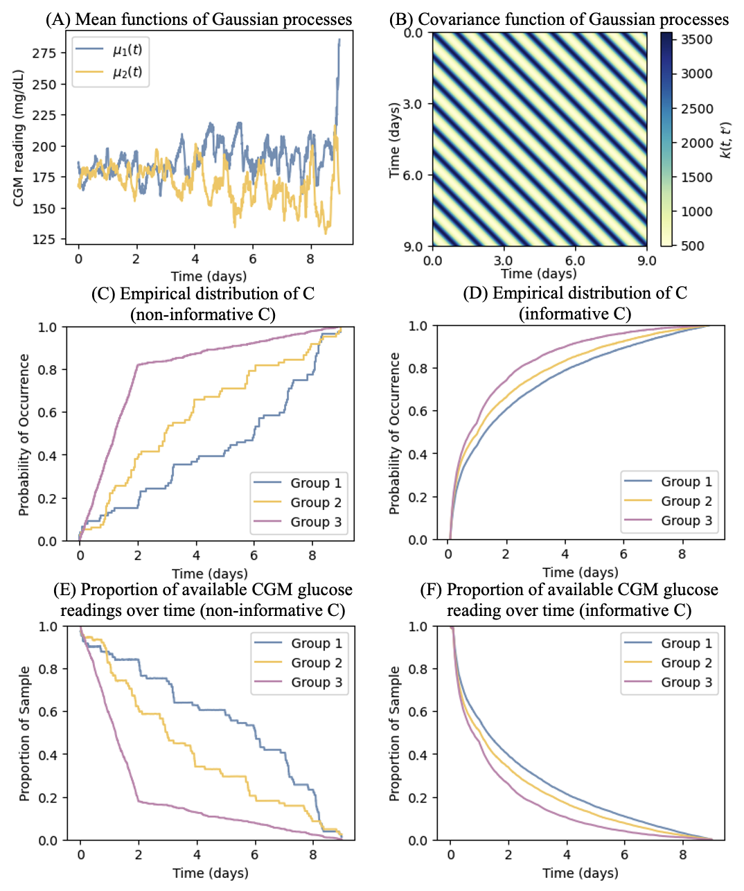
Our data generation scheme closely mimic real data scenarios in inpatient CGM studies. Specifically, we generate CGM glucose trajectories as Gaussian processes, , where denotes the mean function and denotes the covariance function characterized by a periodic kernel that takes the form, . The kernel parameters, amplitude (), length-scale (), and period (), govern the mean deviation, trajectory smoothness, and repetition frequency, respectively. To reflect the natural 1-day (i.e., 1440 minutes) periodicity in glucose, we set the the period , length-scale , and amplitude . The resulting covariance matrix is shown in Figure 1(B).
In each simulation setting, three groups of CGM glucose trajectories are generated and are referred to as Group 1, Group 2, and Group 3. For Groups 1 and 2, the corresponding mean functions, denoted by and , are specified as the empirical mean functions of the CGM glucose trajectories observed for the two study groups considered in the real data application presented in Section 5. For Group 3, we use the same mean function specified for Group 1 so that comparing Group 1 versus Group 3 can serve as the null case with respective to the hypothesis testing on the equivalence in mean TIR. In addition, we set as an equally spaced time grid with the step size of 5 minutes, mimicking the data capturing scheme of a Dexcom G6 CGM system.
To induce missing data for the generated CGM glucose trajectories, we first impose intermittent missing. Specifically, we draw the starting time of the intermittent missing from an exponential distribution with the scale parameter of 3424, which is derived from the real data application discussed in Section 5, and then set the missing duration as a random number generated from a uniform distribution between 10 and 70 (minutes). By doing so, we determine the time interval when the intermittent missing occurs, and subsequently .
Next, we generate , which represents the ending time of CGM, in the following two ways:
(I) is completely non-informative and is sampled from a distribution not related to the generation of glucose trajectories. Specifically, for Groups 1 and 2, we sample ’s with replacement from the empirical distribution of the observed CGM follow-up durations in the real data application discussed in Section 5. For Group 3, ’s are generated from a mixture distribution, , where is the uniform distribution function between 0 to 2 (days) and is the uniform distribution function between 2 and 9 (days).
(II) is informative, depending on the history of glucose trajectories, and is generated from the Cox’s proportional hazards model (4) with , where captures the average glucose during the previous day as of time (which equals when indicates a time point during the first day), and is drawn from a uniform distribution . To make and to range within a similar scale, we normalize by dividing it by .
We let and for Group 1, and for Group 2, and and for Group 3.
With the and obtained as above, we compute the availability indicator , and is observed if and only if . The empirical distribution of and the empirical mean of , which reflects the proportion of the available glucose readings at time , in case (I) and case (II) are plotted in Figure 1(C)–Figure 1(F).
In each simulation setting, we consider sample sizes and , and generate 1000 replicated datasets. The bootstrap based inferences are implemented based on 200 bootstrapping samples.
4.2 Simulation results
In each simulation setting, we analyze the mean TIR over 7 days with the target glucose ranges, mg/dL, between 70 and 180 mg/dL, and mg/dL, using three different methods: (1) the oracle approach that computes based on the fully observed without any missing data; (2) the proposed approach that uses ; (3) the naive approach that completely ignores the missing data and estimates by .
Table 1 summarizes the simulation results in the setting with informative CGM follow-up durations (i.e., ’s). The presented results include the empirical averages, relative biases, empirical standard deviations, and estimated standard errors (based on bootstrapping) of the three different estimators of mean TIR. The relative bias is defined as the absolute difference between the average estimate and the average oracle estimate divided by the average oracle estimate. We also report the empirical rejection rates from testing the mean TIR equivalence between Groups 1 and 2 and between Groups 1 and 3. Since the mean TIRs are the same between Groups 1 and 3 and are different between Groups 1 and 2, the empirical rejection rates in these cases respectively reflect empirical size and empirical power.
From Table 1, we observe that the proposed estimator of mean TIR is virtually unbiased with the relative biases mostly below 5% and exhibiting a decreasing trend with the sample size. The empirical standard deviations and the estimated standard errors closely agree with each other. The naive estimator demonstrates apparent biases in many cases. For example, even when the sample size is as large as 200, the relative biases of the naive estimates for the TIR mg/dL are still pretty substantial, equal to 23.7%, 18.7%, and 33% for Groups 1, 2, and 3 respectively. In contrast, the corresponding relative biases of the proposed estimator are much smaller, equal to 0.4%, 0.1%, and 6.6%. It is noted that the proposed estimator generally produces larger relative biases for Group 3 as compared to that for Group 1, though Group 1 and Group 3 share the same mean TIR. This can be explained by the different distributions of between these two groups (see Figure 1(D)), which entail more frequent early termination of CGM and thus more intensive monotone missing in the data for Group 3 (as confirmed by Figure 1(F)). As expected, the lower proportions of available CGM glucose readings in Group 3 (as compared to Group 1) also result in larger estimation variability captured by either empirical standard deviations or estimated standard errors.
Regarding the hypothesis testing that compares the mean TIR between Groups 1 and 3, the proposed method yields empirical sizes quite close to the nominal significance level of 5%, while the naive approach may be prone to inflated type I errors (e.g., the empirical size of 10% when comparing the mean TIR mg/dL with ). By examining the empirical rejection rates for comparing Groups 1 vs. 2, we find that the test based on the proposed method is much more powerful as compared to the test based on the naive approach, as evidenced by more than two fold larger empirical rejection rates. For example, with the larger sample size 200, the naive method only has around 11% power to detect the difference in mean TIR between Group 1 and Group 2, while the proposed method has 74% power to do so.
The simulation results in the setting with non-informative ’s are presented in Table S1 of Web Appendix B.1. The finding from Table S1 is consistent with that from Table 1. Both suggest that failing to properly account for the special missing features of the inpatient CGM glucose trajectories can lead to considerably biased estimation of mean TIR as well as problematic inferences that are reflected by the inflated type I errors and substantial power loss associated with the naive method.
| Sample size | Target glucose range | |||||||||
|---|---|---|---|---|---|---|---|---|---|---|
| per group | Between and | |||||||||
| n = 50 | Oracle | Naive | Proposed | Oracle | Naive | Proposed | Oracle | Naive | Proposed | |
| Group 1 | AvgEst (%) | 1.18 | 1.45 | 1.2 | 43.26 | 47.18 | 43.4 | 55.26 | 50.97 | 55.1 |
| RelBias (%) | - | 23.3 | 1.4 | - | 9.1 | 0.3 | - | 7.8 | 0.3 | |
| BSE () | 0.51 | 0.64 | 0.66 | 3.74 | 3.94 | 5.64 | 3.94 | 4.14 | 5.89 | |
| ESD () | 0.51 | 0.64 | 0.66 | 3.73 | 3.93 | 5.62 | 3.93 | 4.13 | 5.87 | |
| Group 2 | AvgEst (%) | 2.56 | 2.08 | 2.61 | 51.74 | 49.28 | 51.85 | 44.72 | 47.91 | 44.51 |
| RelBias (%) | - | 18.6 | 1.9 | - | 4.8 | 0.2 | - | 7.1 | 0.5 | |
| BSE () | 0.78 | 0.78 | 1.25 | 3.63 | 3.91 | 5.81 | 3.94 | 4.18 | 6.38 | |
| ESD () | 0.78 | 0.77 | 1.24 | 3.62 | 3.9 | 5.79 | 3.93 | 4.17 | 6.36 | |
| Group 3 | AvgEst (%) | 1.17 | 1.56 | 1.4 | 43.13 | 48.52 | 45.57 | 55.39 | 49.47 | 52.63 |
| RelBias (%) | - | 33.7 | 19.4 | - | 12.5 | 5.7 | - | 10.7 | 5.0 | |
| BSE () | 0.51 | 0.71 | 0.93 | 3.77 | 4.09 | 7.88 | 3.95 | 4.28 | 8.32 | |
| ESD () | 0.51 | 0.7 | 0.91 | 3.76 | 4.08 | 7.52 | 3.94 | 4.27 | 7.95 | |
| Power | Groups 1 vs 2 | 29.4% | 8.2% | 21.3% | 36.6% | 6.9% | 31.6% | 46.7% | 9.1% | 34.4% |
| Size | Groups 1 vs 3 | 4.7% | 6.8% | 4.4% | 5.5% | 9.2% | 6.7% | 5.0% | 9.3% | 6.7% |
| n = 100 | ||||||||||
| Group 1 | AvgEst (%) | 1.18 | 1.47 | 1.16 | 43.33 | 47.26 | 43.24 | 55.16 | 50.85 | 55.26 |
| RelBias (%) | - | 24.6 | 1.3 | - | 9.1 | 0.2 | - | 7.8 | 0.2 | |
| BSE () | 0.37 | 0.47 | 0.5 | 2.67 | 2.81 | 4.03 | 2.81 | 2.96 | 4.22 | |
| ESD() | 0.37 | 0.47 | 0.5 | 2.66 | 2.8 | 4.02 | 2.8 | 2.95 | 4.21 | |
| Group 2 | AvgEst (%) | 2.59 | 2.1 | 2.58 | 51.72 | 49.35 | 51.63 | 44.69 | 47.79 | 44.77 |
| RelBias (%) | - | 18.7 | 0.2 | - | 4.6 | 0.2 | - | 7.0 | 0.2 | |
| BSE () | 0.56 | 0.57 | 0.94 | 2.58 | 2.79 | 4.23 | 2.8 | 2.98 | 4.6 | |
| ESD () | 0.56 | 0.56 | 0.94 | 2.57 | 2.78 | 4.22 | 2.79 | 2.97 | 4.59 | |
| Group 3 | AvgEst (%) | 1.18 | 1.58 | 1.35 | 43.4 | 48.79 | 44.56 | 55.1 | 49.19 | 53.73 |
| RelBias (%) | - | 33.2 | 14.4 | - | 12.4 | 2.7 | - | 10.7 | 2.5 | |
| BSE () | 0.37 | 0.52 | 0.78 | 2.68 | 2.91 | 6.89 | 2.81 | 3.05 | 7.21 | |
| ESD () | 0.37 | 0.52 | 0.76 | 2.67 | 2.91 | 6.58 | 2.8 | 3.05 | 6.88 | |
| Power | Groups 1 vs 2 | 55.8% | 14.4% | 31.5% | 60.2% | 9.8% | 52.2% | 72.7% | 12.7% | 59.3% |
| Size | Groups 1 vs 3 | 4.8% | 7.2% | 6.6% | 6.3% | 9.7% | 7.7% | 6.4% | 9.6% | 6.7% |
| n = 200 | ||||||||||
| Group 1 | AvgEst (%) | 1.19 | 1.48 | 1.19 | 43.39 | 47.32 | 43.38 | 55.09 | 50.78 | 55.1 |
| RelBias (%) | - | 23.7 | 0.3 | - | 9.1 | 0.0 | - | 7.8 | 0.0 | |
| BSE () | 0.27 | 0.34 | 0.38 | 1.89 | 1.99 | 2.89 | 1.99 | 2.09 | 3.02 | |
| ESD () | 0.27 | 0.34 | 0.37 | 1.88 | 1.98 | 2.88 | 1.98 | 2.08 | 3.01 | |
| Group 2 | AvgEst (%) | 2.6 | 2.11 | 2.6 | 51.69 | 49.31 | 51.52 | 44.7 | 47.83 | 44.88 |
| RelBias (%) | - | 18.7 | 0.1 | - | 4.6 | 0.3 | - | 7.0 | 0.4 | |
| BSE () | 0.4 | 0.41 | 0.7 | 1.83 | 1.97 | 3.05 | 2.0 | 2.12 | 3.34 | |
| ESD () | 0.4 | 0.41 | 0.7 | 1.83 | 1.97 | 3.04 | 1.99 | 2.11 | 3.33 | |
| Group 3 | AvgEst (%) | 1.18 | 1.57 | 1.26 | 43.41 | 48.85 | 44.15 | 55.08 | 49.12 | 54.25 |
| RelBias (%) | - | 33.0 | 6.6 | - | 12.5 | 1.7 | - | 10.8 | 1.5 | |
| BSE () | 0.27 | 0.37 | 0.62 | 1.89 | 2.05 | 5.83 | 1.98 | 2.16 | 6.14 | |
| ESD () | 0.27 | 0.37 | 0.61 | 1.89 | 2.05 | 5.61 | 1.98 | 2.15 | 5.9 | |
| Power | Groups 1 vs 2 | 84.4% | 21.1% | 71.3% | 88.4% | 10.6% | 73.7% | 96.0% | 16.0% | 82.1% |
| Size | Groups 1 vs 3 | 5.3% | 7.0% | 6.2% | 6.7% | 9.9% | 7.0% | 6.5% | 10.0% | 6.8% |
4.3 Simulation studies under different configurations
We conduct simulation studies under other configurations that represent different realistic characteristics of inpatient CGM data. For example, we consider settings with different sizes of group difference by modulating the mean functions used to generate CGM glucose trajectories. We also simulate data with different missing data patterns by varying the distributions of . Details on these additional simulation studies are provided in Web Appendix B.2. The results consistently demonstrate the advantages of the proposed method over the naive method.
4.4 Simulation studies on sensitivity analysis
We further conduct simulation studies to evaluate the robustness of the proposed method to the misspecification of the assumed Cox model for given . Specifically, we generate the CGM glucose trajectory as a Gaussian process with the mean function and the covariance function , which is the same as that plotted in Figure 1(B). We set the mean function for Group 1 or 3 and for Group 2, where and are the same as those plotted in Figure 1(A) and is a random variable. We generate the ending time of CGM, , based on a transformation model (Cheng et al., 1995), , where for Group 1 and Group 2 and for Group 3, and the error term has the distribution function, . Here denotes the standard logistic distribution function and denotes the extreme value distribution function. It is clear that follows the Cox proportional hazards model (4) with when and a proportional odds model when . As such, the magnitude of the parameter reflects the degree of departure from a Cox model.
Table 2 presents the simulation results for the settings described above with and . It is shown that the proposed method yields quite small relative biases, ranging from 1.2% to 2.0%, when or . The empirical sizes for testing the mean TIR equivalence between Group 1 and Group 3 are still quite close to the nominal significance level of . At the same time, the relative biases of the naive estimator are several fold larger than those of the proposed estimator. The naive method also results in tests which yield inflated type-I errors or suffer from substantial power loss. These observations suggest that the proposed method can offer robust estimation and inference on mean TIR and consistently outperform the naive method even when the Cox model assumption for the CGM follow up duration (i.e., ) does not hold.
| Degree of departure | Sample size | Target glucose range | ||||||||
|---|---|---|---|---|---|---|---|---|---|---|
| from a Cox model | per group | Between and | ||||||||
| p = 0.5 | n = 200 | Oracle | Naive | Proposed | Oracle | Naive | Proposed | Oracle | Naive | Proposed |
| Group 1 | AvgEst (%) | 1.26 | 1.5 | 1.24 | 44.47 | 47.51 | 43.76 | 53.92 | 50.56 | 54.73 |
| RelBias (%) | - | 19.1 | 1.9 | - | 6.8 | 1.6 | - | 6.2 | 1.5 | |
| BSE () | 0.28 | 0.37 | 0.33 | 1.89 | 2.07 | 2.39 | 1.99 | 2.16 | 2.51 | |
| ESD () | 0.28 | 0.37 | 0.33 | 1.9 | 2.08 | 2.4 | 1.99 | 2.17 | 2.51 | |
| Group 2 | AvgEst (%) | 2.43 | 2.15 | 2.49 | 50.85 | 49.39 | 51.56 | 45.8 | 47.7 | 45.07 |
| RelBias (%) | - | 11.7 | 2.7 | - | 2.9 | 1.4 | - | 4.1 | 1.6 | |
| BSE () | 0.39 | 0.43 | 0.51 | 1.84 | 2.03 | 2.32 | 2.0 | 2.17 | 2.51 | |
| ESD () | 0.39 | 0.43 | 0.51 | 1.84 | 2.04 | 2.33 | 2.0 | 2.17 | 2.52 | |
| Group 3 | AvgEst (%) | 1.27 | 1.64 | 1.24 | 44.29 | 48.83 | 43.4 | 54.08 | 49.05 | 55.11 |
| RelBias (%) | - | 28.9 | 2.4 | - | 10.2 | 2.0 | - | 9.3 | 1.9 | |
| BSE () | 0.28 | 0.43 | 0.43 | 1.89 | 2.24 | 3.18 | 1.99 | 2.34 | 3.34 | |
| ESD () | 0.28 | 0.44 | 0.43 | 1.9 | 2.25 | 3.19 | 2.0 | 2.34 | 3.35 | |
| Power | Groups 1 vs 2 | 69.4% | 22.2% | 57.3% | 68.8% | 9.6% | 59.6% | 83.0% | 14.6% | 74.5% |
| Size | Groups 1 vs 3 | 4.6% | 7.8% | 5.3% | 6.0% | 10.3% | 4.8% | 5.4% | 9.7% | 4.6% |
| p = 1 | n = 200 | Oracle | Naive | Proposed | Oracle | Naive | Proposed | Oracle | Naive | Proposed |
| Group 1 | AvgEst (%) | 1.27 | 1.49 | 1.26 | 44.35 | 47.07 | 43.7 | 54.01 | 51.01 | 54.79 |
| RelBias (%) | - | 17.0 | 1.2 | - | 6.1 | 1.5 | - | 5.6 | 1.5 | |
| BSE () | 0.28 | 0.36 | 0.33 | 1.9 | 2.07 | 2.31 | 2.0 | 2.16 | 2.44 | |
| ESD () | 0.28 | 0.36 | 0.33 | 1.89 | 2.06 | 2.31 | 1.99 | 2.16 | 2.44 | |
| Group 2 | AvgEst (%) | 2.47 | 2.22 | 2.51 | 50.98 | 49.77 | 51.67 | 45.6 | 47.2 | 44.89 |
| RelBias (%) | - | 10.1 | 1.7 | - | 2.4 | 1.4 | - | 3.5 | 1.6 | |
| BSE () | 0.39 | 0.43 | 0.49 | 1.85 | 2.03 | 2.24 | 2.0 | 2.17 | 2.45 | |
| ESD () | 0.39 | 0.43 | 0.49 | 1.84 | 2.03 | 2.23 | 2.0 | 2.17 | 2.44 | |
| Group 3 | AvgEst (%) | 1.26 | 1.58 | 1.22 | 44.28 | 48.37 | 43.46 | 54.11 | 49.59 | 55.06 |
| RelBias (%) | - | 25.9 | 3.3 | - | 9.2 | 1.9 | - | 8.3 | 1.8 | |
| BSE () | 0.28 | 0.43 | 0.38 | 1.89 | 2.23 | 2.84 | 1.99 | 2.33 | 2.98 | |
| ESD () | 0.28 | 0.42 | 0.38 | 1.89 | 2.23 | 2.83 | 1.99 | 2.32 | 2.97 | |
| Power | Groups 1 vs 2 | 70.4% | 27.2% | 55.6% | 71.7% | 15.7% | 60.7% | 85.1% | 23.1% | 74.7% |
| Size | Groups 1 vs 3 | 4.5% | 6.2% | 5.4% | 6.1% | 8.8% | 5.3% | 5.3% | 9.2% | 5.8% |
5 A Real Data Application
We apply the proposed method to a combined dataset from two inpatient CGM studies, Dexcom G6 Observational Study (Davis et al., 2021) and Dexcom G6 Interventional Study (Spanakis et al., 2022). Dexcom G6 Observational Study was an observational study of 91 insulin-treated adult medicine and surgery patients with type 2 diabetes, aiming to evaluate the feasibility of using the Dexcom G6 CGM in hospitals. Dexcom G6 Interventional Study was a randomized multi-center clinical trial which was aimed to assess the efficacy of Dexcom G6 CGM in guiding insulin adjustment in insulin-treated adult medicine and surgery patients with diabetes. Among the 185 patients who consented to participate in this study, 91 patients were randomized to receive the standard of care with insulin dose adjusted based on capillary point-of care glucose monitoring while wearing a blinded Dexcom G6 CGM (i.e., control group), and 94 patients were randomized to receive insulin adjustment based on daily CGM profile (i.e., intervention group). The Dexcom G6 Observational Study and the Dexcom G6 Interventional Study adopted the same inclusion and exclusion criteria for study enrollment and the same standard of care protocol, which was implemented for all participants of Dexcom G6 Observational Study and the control group of Dexcom G6 Interventional Study. After pooling the datasets from these two inpatient CGM studies, we use the combined dataset to evaluate the effect of CGM-guided insulin adjustment on various TIR outcomes.
In our analyses, the TIR outcomes of interest include TIR defined for six glycemic ranges, mg/dL, between and mg/dL, between and mg/dL, mg/dL, mg/dL, and mg/dL, and over time periods of , , , and days. The ranges of 70–180 mg/dL and 70–140 mg/dL represent two commonly adopted glycemic control targets in hospitals with the latter one being more strict than the former one. The ranges of mg/dL, mg/dL, and mg/dL respectively correspond to borderline hyperglycemia, hyperglycemia, and severe hyperglycemia. The range of mg/dL is considered to mark the time under mild hypoglycemia. After removing patients who had less than 24 hours of hospital stay, the final dataset includes 249 patients with 167 patients in the control group and 82 patients in the intervention group.
The summary statistics with respect to age, gender, race, BMI, and obesity status are presented in Table S4 of Web Appendix B, showing similar patient characteristics between the intervention group and the control group. From Table S4, we observe a trend of longer CGM follow-up duration for the control group as compared to the intervention group (e.g., median CGM follow-up duration of 91.8 vs. 71.0 hours). The shorter CGM follow-up durations, which implicate shorter lengths of hospital stay, in the intervention group may be related to better glycemic control resulted from the CGM-guided intervention; hence ’s in this dataset are likely informative about the underlying glycemic control. The proposed method can properly account for such informative ’s by allowing to depend on CGM glucose history.
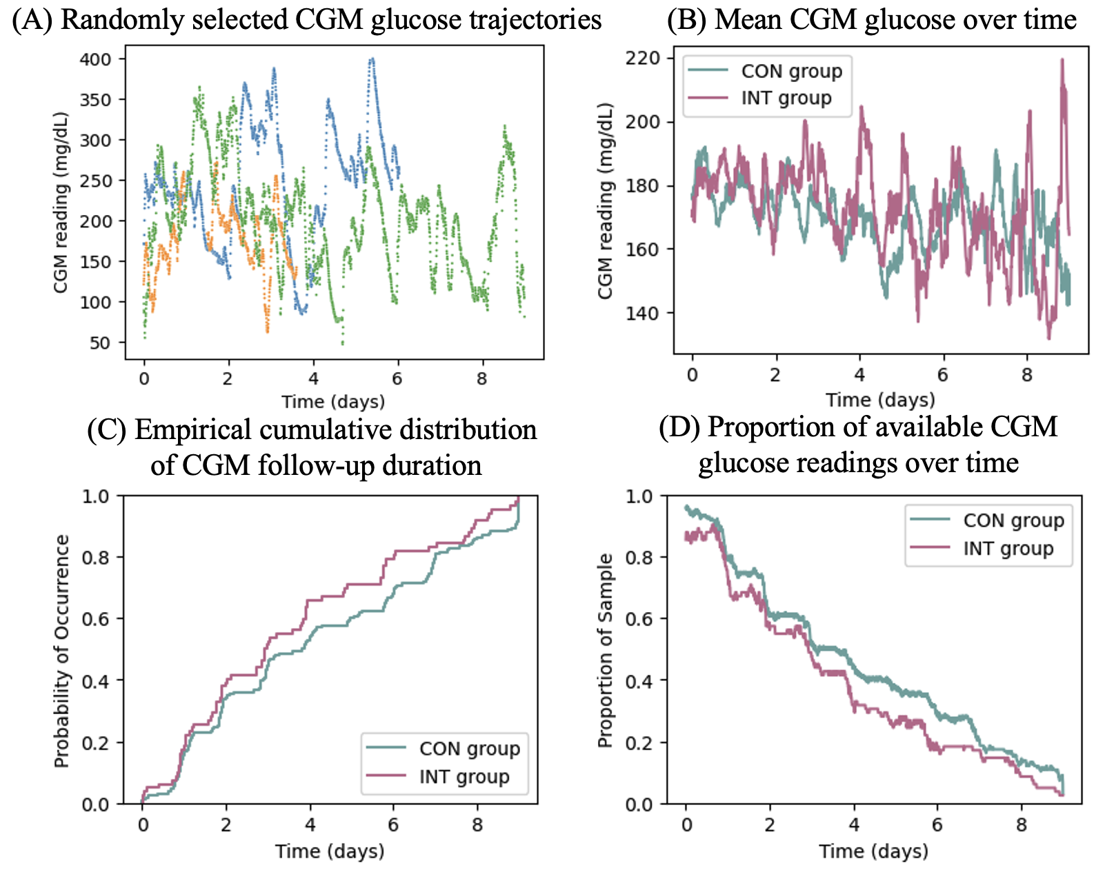
In Figure 2, we illustrate and summarize the CGM glucose trajectories in our dataset. Figure 2(A) presents three randomly selected CGM glucose trajectories. These trajectories shows the heterogeneous temporal patterns across individuals as well as the subject-varying follow-up duration of CGM. Figure 2(B) presents the average CGM glucose readings over time for the control group and the interventional group, which entail the overall non-stationary patterns of inpatient CGM glucose trajectories. In Figure 2(C), we plot the empirical distributions of CGM follow-up duration separately for the control group and the intervention group, suggesting a trend of shorter CGM follow-up durations in the intervention group which result in lower proportions of available CGM glucose reading over time, as shown in Figure 2(D).
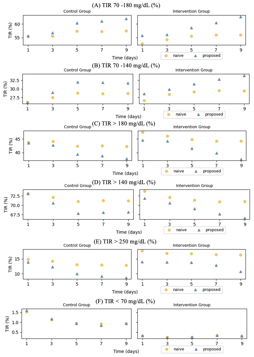
In Figure 3, we present the proposed estimates and the naive estimates for the mean TIR outcomes described earlier, which correspond to with , , , , , and (days), separately for the control and intervention groups. We observe notable discrepancies between the proposed estimates and the naive estimates. For mean TIR 70-180 mg/dL and mean TIR 70-140 mg/dL, the proposed estimates are generally larger than the naive estimates. This is well expected because of a typical inpatient glucose pattern of being higher (and then more out-of-target glucose values) at the beginning of a hospital stay and gradually stabilized over time. The naive method takes the CGM glucose pattern observed for a hospital stay shorter than the required amount of time as the representative pattern for the whole time period. Doing so essentially overweighs the lower within-target proportions inherited with the initial CGM period in hospital, and thus yields a mean TIR estimate biased downwards. The same explanation can be adapted to explain the lower estimated TIR by the proposed method (as compared to the naive estimate) with the glycemic ranges being above 140, 180, or 250 mg/dL. As the patient cohorts of the Dexcom G6 Observation and Interventional Studies generally have small TIR mg/dL, the differences between the proposed estimates and the naive estimates for the corresponding mean TIR have small magnitudes, as shown by Figure 3.
We compare the mean TIR outcomes between the control group and the intervention group. In Table 3, we present the estimates and the corresponding standard errors for mean TIRs with (days) as well as the p values for testing the mean TIR equivalence between the two groups (which are obtained by bootstrapping). The proposed and naive methods attain similar conclusions regarding the comparisons of mean TIRs between the control and intervention groups. The results from both methods suggest similar mean TIRs for the glycemic targets of mg/dL and mg/dL, and the ranges of above , and mg/dL between the control and intervention groups. At the same time, applying the proposed method yields the estimated mean TIR for the intervention group equal to 0.34%, which is much lower than that for the control group, which equals 0.84%. The value for comparing the mean TIR between these two groups is . This result confirms the previous finding that CGM guided insulin adjustment may help reduce the percent time in hypoglycemia (Spanakis et al., 2022). Through properly handling the incompletely observed CGM glucose trajectories over the first 7 days which are commonly presented in our dataset, the proposed analysis evidences the benefit of CGM in hypoglycemia prevention and correction with enhanced statistical rigor.
The proposed estimation and inference regarding the TIR outcomes over 1, 3, 5, 9 days yield consistent findings. The detailed results are provided in Tables S5-S8 of Web Appendix B. The consistent findings across the TIR outcomes defined with different CGM lengths consolidate the conclusions drawn from our analyses.
| Naive Method | |||
| Control group (N = 167) | Intervention group (N = 82) | P value a | |
| TIR 70 - 180 mg/dL (%) | 57.332.14 | 56.053.48 | 0.75 |
| TIR 70 - 140 mg/dL (%) | 28.631.88 | 29.532.78 | 0.79 |
| TIR 180 mg/dL (%) | 42.452.15 | 44.173.31 | 0.66 |
| TIR 140 mg/dL (%) | 71.281.84 | 70.922.86 | 0.92 |
| TIR 250 mg/dL (%) | 12.971.4 | 16.482.67 | 0.24 |
| TIR 70 mg/dL (%) | 0.910.16 | 0.340.1 | 0.01 |
| Proposed Method | |||
| TIR 70 - 180 mg/dL (%) | 61.062.12 | 60.433.92 | 0.89 |
| TIR 70 - 140 mg/dL (%) | 31.922.18 | 32.763.53 | 0.84 |
| TIR 180 mg/dL (%) | 38.812.23 | 39.813.84 | 0.82 |
| TIR 140 mg/dL (%) | 68.152.18 | 67.713.48 | 0.92 |
| TIR 250 mg/dL (%) | 9.160.99 | 12.832.45 | 0.17 |
| TIR 70 mg/dL (%) | 0.840.15 | 0.340.14 | 0.01 |
-
a
The p values are calculated using the Wald-type test described in Section 3.
6 Remarks
This work represents a timely effort to develop rigorous statistical estimation and inference tools for the analysis of inpatient CGM studies which are on a rapid rise since the Covid-19 pandemic. Through formulating the real CGM glucose data as functional data subject to missing, we develop viable and robust statistical strategies to deal with the special data features inherited with inpatient CGM studies, which however are commonly ignored in routine data analyses. Our proposals have solid theoretical underpinning while enjoying simple and stable implementation. The Python code for implementing the proposed method is publicly available on the GitHub repository: https://github.com/qyxxx/CGM_meanTIR. Future development may involve an R version. Such updates will be made available on the same GitHub repository.
Acknowledgements
The proposed research has been sponsored by the funding from the National Institutes of Health (Grant No.: R01DKDK136023).
Supplementary Materials
References
- Aalen (1980) Aalen, O. (1980). A model for nonparametric regression analysis of counting processes. In Mathematical Statistics and Probability Theory: Proceedings, Sixth International Conference, Wisła (Poland), 1978, pages 1–25. Springer.
- Al-Harbi et al. (2022) Al-Harbi, M. Y., Albunyan, A., Alnahari, A., Kao, K., Brandner, L., El Jammal, M., and Dunn, T. C. (2022). Frequency of flash glucose monitoring and glucose metrics: real-world observational data from saudi arabia. Diabetology & Metabolic Syndrome 14, 66.
- Andersen and Gill (1982) Andersen, P. K. and Gill, R. D. (1982). Cox’s regression model for counting processes: a large sample study. The annals of statistics pages 1100–1120.
- Austin (2022) Austin, P. C. (2022). Bootstrap vs asymptotic variance estimation when using propensity score weighting with continuous and binary outcomes. Statistics in Medicine 41, 4426–4443.
- Capaldo et al. (2020) Capaldo, B., Annuzzi, G., Creanza, A., Giglio, C., De Angelis, R., Lupoli, R., Masulli, M., Riccardi, G., Rivellese, A. A., and Bozzetto, L. (2020). Blood glucose control during lockdown for covid-19: Cgm metrics in italian adults with type 1 diabetes. Diabetes Care 43, e88.
- Castañeda et al. (2022) Castañeda, J., Mathieu, C., Aanstoot, H.-J., Arrieta, A., Da Silva, J., Shin, J., and Cohen, O. (2022). Predictors of time in target glucose range in real-world users of the minimed 780g system. Diabetes, Obesity and Metabolism 24, 2212–2221.
- Cheng et al. (1995) Cheng, S., Wei, L. J., and Ying, Z. (1995). Analysis of transformation models with censored data. Biometrika 82, 835–845.
- Cuesta-Frau et al. (2018) Cuesta-Frau, D., Novák, D., Burda, V., Molina-Picó, A., Vargas, B., Mraz, M., Kavalkova, P., Benes, M., and Haluzik, M. (2018). Characterization of artifact influence on the classification of glucose time series using sample entropy statistics. Entropy 20, 871.
- Davis et al. (2021) Davis, G. M., Spanakis, E. K., Migdal, A. L., Singh, L. G., Albury, B., Urrutia, M. A., Zamudio-Coronado, K. W., Scott, W. H., Doerfler, R., Lizama, S., et al. (2021). Accuracy of dexcom g6 continuous glucose monitoring in non–critically ill hospitalized patients with diabetes. Diabetes Care 44, 1641–1646.
- diaTribe Foundation (2022) diaTribe Foundation, T. (2022). New international consensus on cgm clinical trial metrics aims to spur diabetes treatment advances. https://www.prnewswire.com/news-releases/new-international-consensus-on-cgm-clinical-trial-metrics-aims-to-spur-diabetes-treatment-advances-301695977.html .
- Gecili et al. (2021) Gecili, E., Huang, R., Khoury, J. C., King, E., Altaye, M., Bowers, K., and Szczesniak, R. D. (2021). Functional data analysis and prediction tools for continuous glucose-monitoring studies. Journal of Clinical and Translational Science 5, e51.
- Klarskov et al. (2022) Klarskov, C. K., Windum, N. A., Olsen, M. T., Dungu, A. M., Jensen, A. K., Lindegaard, B., Pedersen-Bjergaard, U., and Kristensen, P. L. (2022). Telemetric continuous glucose monitoring during the covid-19 pandemic in isolated hospitalized patients in denmark: a randomized controlled exploratory trial. Diabetes Technology & Therapeutics 24, 102–112.
- Kosorok (2008) Kosorok, M. R. (2008). Introduction to empirical processes and semiparametric inference, volume 61. Springer.
- Lin (2007) Lin, D. (2007). On the breslow estimator. Lifetime data analysis 13, 471–480.
- Linden et al. (2021) Linden, J., Welsh, J., Hirsch, I., and Garg, S. (2021). Real-time continuous glucose monitoring during the coronavirus disease 2019 pandemic and its impact on time in range. Diabetes Technol Ther 23, S–1.
- Mayeda et al. (2020) Mayeda, L., Katz, R., Ahmad, I., Bansal, N., Batacchi, Z., Hirsch, I. B., Robinson, N., Trence, D. L., Zelnick, L., and De Boer, I. H. (2020). Glucose time in range and peripheral neuropathy in type 2 diabetes mellitus and chronic kidney disease. BMJ open diabetes research & care 8,.
- Olsen et al. (2022) Olsen, M. T., Dungu, A. M., Klarskov, C. K., Jensen, A. K., Lindegaard, B., and Kristensen, P. L. (2022). Glycemic variability assessed by continuous glucose monitoring in hospitalized patients with community-acquired pneumonia. BMC Pulmonary Medicine 22, 83.
- Olsen et al. (2024) Olsen, M. T., Klarskov, C. K., Dungu, A. M., Hansen, K. B., Pedersen-Bjergaard, U., and Kristensen, P. L. (2024). Statistical packages and algorithms for the analysis of continuous glucose monitoring data: A systematic review. Journal of diabetes science and technology page 19322968231221803.
- Peng and Fine (2007) Peng, L. and Fine, J. P. (2007). Regression modeling of semicompeting risks data. Biometrics 63, 96–108.
- Raj et al. (2022) Raj, R., Mishra, R., Jha, N., Joshi, V., Correa, R., and Kern, P. A. (2022). Time in range, as measured by continuous glucose monitor, as a predictor of microvascular complications in type 2 diabetes: a systematic review. BMJ Open Diabetes Research & Care 10,.
- Smarr et al. (2020) Smarr, B. L., Aschbacher, K., Fisher, S. M., Chowdhary, A., Dilchert, S., Puldon, K., Rao, A., Hecht, F. M., and Mason, A. E. (2020). Feasibility of continuous fever monitoring using wearable devices. Scientific reports 10, 21640.
- Spanakis et al. (2022) Spanakis, E. K., Urrutia, A., Galindo, R. J., Vellanki, P., Migdal, A. L., Davis, G., Fayfman, M., Idrees, T., Pasquel, F. J., Coronado, W. Z., et al. (2022). Continuous glucose monitoring–guided insulin administration in hospitalized patients with diabetes: a randomized clinical trial. Diabetes Care 45, 2369–2375.
- Vaart and Wellner (2023) Vaart, A. v. d. and Wellner, J. A. (2023). Empirical processes. In Weak Convergence and Empirical Processes: With Applications to Statistics, pages 127–384. Springer.
- Walsh III et al. (2014) Walsh III, J. A., Topol, E. J., and Steinhubl, S. R. (2014). Novel wireless devices for cardiac monitoring. Circulation 130, 573–581.
- Wilson et al. (2023) Wilson, D. M., Pietropaolo, S. L., Acevedo-Calado, M., Huang, S., Anyaiwe, D., Scheinker, D., Steck, A. K., Vasudevan, M. M., McKay, S. V., Sherr, J. L., et al. (2023). Cgm metrics identify dysglycemic states in participants from the trialnet pathway to prevention study. Diabetes care 46, 526–534.