Tiny-Sepformer: A Tiny Time-Domain Transformer Network for Speech Separation
Abstract
Time-domain Transformer neural networks have proven their superiority in speech separation tasks. However, these models usually have a large number of network parameters, thus often encountering the problem of GPU memory explosion. In this paper, we proposed Tiny-Sepformer, a tiny version of Transformer network for speech separation. We present two techniques to reduce the model parameters and memory consumption: (1) Convolution-Attention (CA) block, spliting the vanilla Transformer to two paths, multi-head attention and 1D depthwise separable convolution, (2) parameter sharing, sharing the layer parameters within the CA block. In our experiments, Tiny-Sepformer could greatly reduce the model size, and achieves comparable separation performance with vanilla Sepformer on WSJ0-2/3Mix datasets.
Index Terms: transformer, separable convolution, parameter sharing, speech separation, tiny ML
1 Introduction
Single-channel multi-speaker speech separation is a significant speech task in real-world applications. Robust speech separation could improve the performance of downstream tasks, such as speaker identification, speech recognition, etc [1, 2]. However, speech separation is a difficult task, often known as the cocktail-party problem [3]. People have made great efforts on deep learning models [4, 5, 6, 7, 8], which were proposed to advance the progress of this tough task.
Traditional speech separation approaches often transform the mixture signals to time-frequency domain and estimate the clean spectrogram of each speaker from the mixture spectrogram. TasNet [9] directly models the audio signal in the time-domain. Conv-TasNet [10] replaces the LSTM of TasNet with 1-D dilated convolutions and it stacks deep convolutional blocks, to model the long-term dependency [11, 12]. To promote the efficiency of handling long time-domain sequence, dual-path frameworks were presented. DPRNN [13] splits the sequence into small chunks, and applies intra and inter chunk operations iteratively. DPTNet [14] introduces Transformer into the recurrent network of DPRNN, and outperforms the vanilla DPRNN. Sepformer [15] was proposed as a RNN-free neural network. The intra and inter chunk operations of masking network are solely based on Transformer, to capture both local and long-term information.
Despite the remarkable achivements of the above Transformer models, they still encounter with some tough problems. One is that they usually have large network parameters, thus often resulting in GPU memory explosion. In this work, we focus on the reduction of network parameters and GPU memory consumption.
Recently, many memory or time efficient attention-based models have been proposed. In Linformer [16], the self-attention mechanism is approximated by a low-rank matrix, resulting a linear complexity Transformer. Performer [17] used a FAVOR+ method to model kernelizable attention mechanism efficiently, instead of sparsity or low-rankness. DF-Conformer [18] integrates Conformer [19] layers with FAVOR+ mechanism into the mask prediction network of Conv-TasNet. Most of these works implemented a efficient system by reducing the self-attention from quadratic to linear complexity, but still have a large amount of model parameters.
In this work, inspired by Lite-Transformer [20], we used Convolution-Attention (CA) block into the masking network, which splits the layer into convolution path and attention path parallelly. The convolution path has much less parameters than the attention path. Moreover, the convolution part of CA is 1D separable convolution [21], which could further reduce the computation. Besides the separable convolution, we also applied parameter sharing technique [22, 23]. All of the layer parameters within one IntraCA/InterCA network are shared, but we do not share the parameters across different IntraCA/InterCA networks. In summary, our proposed Tiny-Sepformer has two major contributions to speech separation: (1) CA network, (2) parameter sharing.
2 Tiny-Sepformer
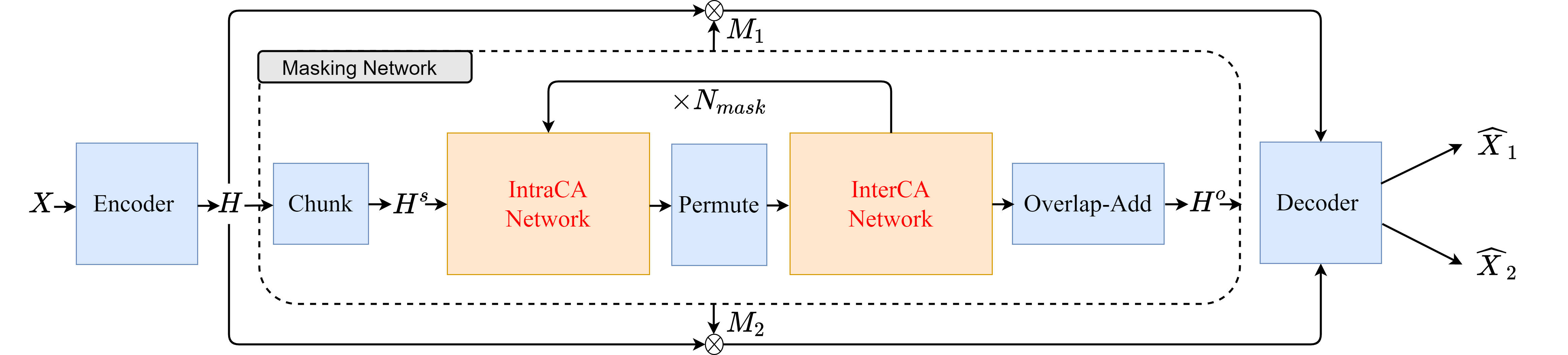
In this work, we propose the Tiny-Sepformer, a tiny Transformer network for speech separation. Tiny-Sepformer is a time-domain masking approach, and is composed of three modules: (1) an encoder , making convolutions on time-domain mixture-signal to the feature representation , where is the length of time-domian signal, (2) a masking network , employing dual-path tiny Convolution-Attention (CA) blocks on , to estimate mask matrices for each of the speakers in the mixture-signal, and (3) a decoder , reconstructing the separated signals in the time domain by multiplicating the masks with for each of the speaker.
2.1 Model Architecture
The overall model architecture is depicted in Figure 1. The time-domain mixture-signal is firstly fed into the encoder . The encoder is a single 1D-convolutional layer, followed by ReLU activation. The hidden feature representation is extracted through the encoder.
| (1) |
After that, the encoder output is used as the input of the masking network , to produce mask matrices .
| (2) |
Finally, the mask matrices and hidden features of encoder are as the input of the decoder . The decoder is a transposed convolutional layer with the same stride and kernel size of the encoder . The decoder outputs the separated signal from each source .
| (3) |
In which, is the transposed convolution, and is denoted as element-wise multiplication. The objective of model training is maximizing the Scale-Invariant Source-to-Noise Ratio (SI-SNR). We use Utterance-level Permutation Invariant Training (uPIT) [24, 25] loss during training to deal with the label permutation problem.
2.2 Masking Network
The masking network consists of three steps: (1) pre-processing and chunking, (2) the proposed tiny Convolution-Attention (CA) blocks , and (3) post-processing and overlap-add.
Firstly, the encoder feature sequence is normalized with layer normalization, and processed by a linear layer to produce the with dimension .
| (4) |
After pre-processing, the hidden feature sequence is processed by the segmentation operation. The segmentation splits two dimensional into three dimensional chunks with overlap. In which, is the chunk size of segmentation, and is the chunk number of segmentation result. The chunked is fed into several CA blocks , which will be detailed in Section 2.3. The CA blocks will be performed by times iteratively to produce .
| (5) |
The output of CA block remains the same dimension with the input . Then, is processed by a linear layer with dimension and with using the PReLU activation.
| (6) |
This post-processing operation generates feature maps for each of the speakers. Afterwards, the Overlap-Add [13] is operated on , merging the three dimensional chunked sequence into two dimensinal feature sequence .
| (7) |
At the end, this representation is through two linear layers and a ReLU activation to obtain the mask matrices for each of the speakers. The dimension of each mask is .
2.3 Convolution-Attention (CA) Block
The Convolution-Attention (CA) Block is the core module of masking network. There are two kinds of network in the masking network: (1) IntraCA network , operating within each chunk to model local features, (2) InterCA network , processing between all the chunks to capture long dependency. The block are designed to process network firstly, then permute the feature dimension from to , and process network at last.
| (8) | ||||
In which, is denoted as the permutation operation. IntraCA is performed times, and InterCA will perform by times iteratively.
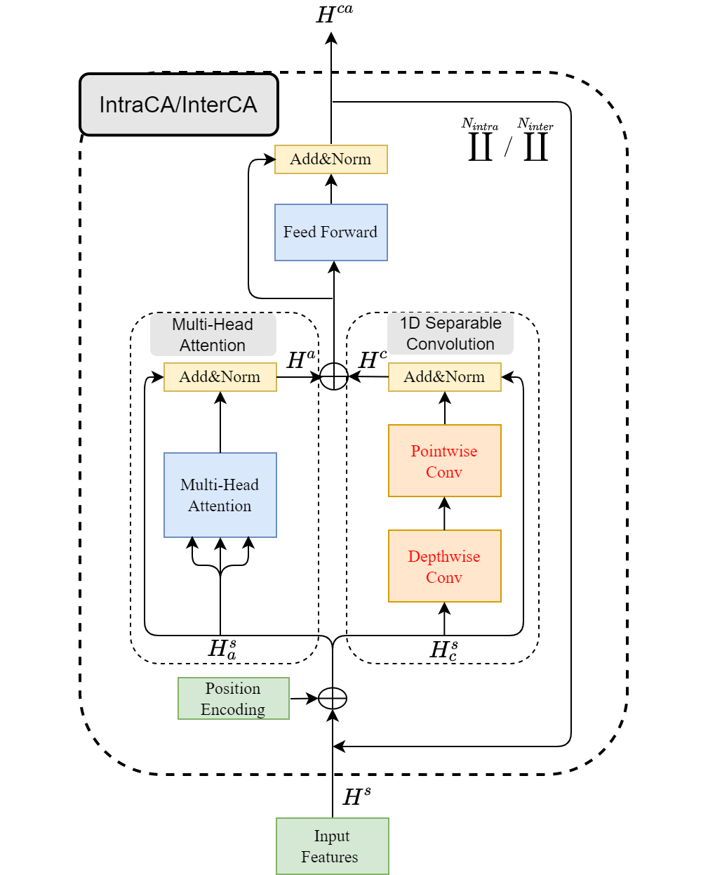
As depicted in Figure 2, IntraCA or InterCA network contains two parts: (1) multi-head attention, (2) 1D depthwise separable convolution. IntraCA and InterCA have the same network structure, but have different network parameters. Taking IntraCA as the example, the input feature is split into two paths: (1) attention feature , and (2) convolution feature , where . The choices of and will be analyzed in Section 3.4. The attention feature is fed into the standard multi-head attention mechanism, followed by layer normalization.
| (9) |
Mean while, the other branch is processed by the 1D depthwise separable convolution as follows:
| (10) |
| (11) |
followed by residual addition and layer normalization.
| (12) |
The 1D depthwise separable convolution could dramaticly reduce the number of network parameters. In addition, the dimension reduction of multi-head attention could also make a light attention layer.
After that, the output of two path and are concatenated together, feeding into feed-forward layers as follows:
| (13) |
In which, is denoted as concatenated operation. The dimension of feed-forward layer is denoted as . Following the feed-forward layer are residual addition and layer normalization, similar to the vanilla Transformer network.
| (14) |
2.4 Parameter Sharing
Another idea of parameters reduction is cross-layer parameter sharing. There are several methods of sharing parameters, such as sharing the feed-forward network parameters, or only sharing attention and convolution parameters. In this work, we propose to share all the layer parameters within IntraCA/InterCA network, but different IntraCA/InterCA networks have different parameters. Therefore, with parameter sharing, the Equation 8 is modified as following:
| (15) |
In which, means that performing the network layer by times iteratively, but each iteration has the same layer parameters. With this approach, the parameters of could decrease to of the original network, as well as the parameters for . We share all the layers in IntraCA and InterCA respectively, resulting in much fewer network parameters of the Tiny-Sepformer model.
2.5 Compared with Conformer
The most relevant structure to CA block is Conformer [19], which connects the attention and convolution in serial. The motivation of our work is to reduce the model parameters. Therefore, we design to connect the multi-head attention and 1D depthwise separable convolution in parallel. For simplicity, in this section, we denoted the input feature of the block as , where is the number of time steps and is the channel dimension. Then, the parameters of attention and convolution paths are as Table 1:
| Network | Parameters |
|---|---|
| Multi-Head Attention | |
| 1D Depthwise Separable Convolution | |
| Attention+Convolution in Serial (Conformer) | |
| Attention+Convolution in Parallel (CA) |
The query, key, value and multi-head projection matrix has parameters respectively. Thus, for multi-head attention, the parameters are . The separable convolution has a depthwise convolutional layer with kernel size on each channel individually, and a pointwise convolutional layer on each frame independently but across all channels . Therefore, for separable convolution, the parameters are . If connecting Attention+Convolution in Serial (Conformer) and keeping the feature dimension as , their parameters are added together (). For our CA block (Attention+Convolution in Parallel), the input feature is split into two branches: . In Table 1, we set for simplicity, then the parameters are reduced to . Through the channel division operation, the parameters of CA block are much less than vanilla Transformer and Conformer, and still keep the feature dimension as into next feedforward layer.
3 Experiment
3.1 Dataset
We use the WSJ0-2mix and WSJ0-3mix [26] datasets to evaluate our Tiny-Sepformer model. These two datasets were generated by randomly selecting utterances from the WSJ0 corpus, and mixing them with two and three speakers. hours of training, hours of validation and hours of test speech dataset were used for all the experiments. All the speech were downsampled to kHz in the data pre-processing.
| Model | WSJ0-2Mix | WSJ0-3Mix | Sharing | Param | |||||
| SI-SNRi | SDRi | SI-SNRi | SDRi | ||||||
| Sepformer-16 [15] | 2 | 4 | 4 | 14.08 | 15.01 | 12.29 | 13.19 | No | 13.0M |
| Sepformer-32 [15] | 2 | 8 | 8 | 15.08 | 16.04 | 12.67 | 13.71 | No | 25.7M |
| Sepformer-32 [15] | 4 | 4 | 4 | 15.07 | 16.02 | 13.02 | 14.01 | No | 25.7M |
| Tiny-Sepformer-16 | 2 | 4 | 4 | 14.29 | 15.13 | 12.87 | 13.85 | No | 10.2M |
| Tiny-Sepformer-32 | 2 | 8 | 8 | 15.09 | 16.03 | 14.38 | 15.36 | No | 20.0M |
| Tiny-Sepformer-32 | 4 | 4 | 4 | 15.10 | 16.07 | 14.50 | 15.53 | No | 20.0M |
| Tiny-SepformerS-16 | 2 | 4 | 4 | 13.51 | 14.22 | 12.38 | 13.21 | Yes | 2.9M |
| Tiny-SepformerS-32 | 2 | 8 | 8 | 14.66 | 15.39 | 12.77 | 13.63 | Yes | 2.9M |
| Tiny-SepformerS-32 | 4 | 4 | 4 | 15.16 | 15.98 | 13.91 | 14.79 | Yes | 5.3M |
| Model | IntraCA | InterCA | WSJ0-2Mix | |
| , | , | SI-SNRi | SDRi | |
| Tiny-Sepformer-32 | 128, 128 | 128, 128 | 15.10 | 16.07 |
| Tiny-Sepformer-32 | 192, 64 | 64, 192 | 15.46 | 16.36 |
| Tiny-Sepformer-32 | 64, 192 | 192, 64 | 14.97 | 15.87 |
| Tiny-SepformerS-32 | 128, 128 | 128, 128 | 15.16 | 15.98 |
| Tiny-SepformerS-32 | 192, 64 | 64, 192 | 15.21 | 16.06 |
| Tiny-SepformerS-32 | 64, 192 | 192, 64 | 15.13 | 15.95 |
3.2 Model Configuration
We conducted all the experiments using the SpeechBrain toolkit [27]. For encoder , the 1D-convolutional layer has filters, a kernel size of , and a stride factor of . For masking network , the dimension of pre-processing is . The segmentation splits the chunks with chunk size with overlap. For decoder , the transposed convolutional layer has the same kernel size and stride factor with the encoder.
3.3 Result
In our experiments, Scale-Invariant Source-to-Noise Ratio improvement (SI-SNRi) and Signal-to-Distortion Ratio improvement (SDRi) [31] are used as the evaluating metrics. As listed in Table 2, we firstly explored different configuration of CA blocks number , IntraCA layers number , and InterCA layers number . The results indicated that our Tiny-Sepformer models achieve comparable separation performance with vanilla Sepformer on both WSJ0-2mix and WSJ0-3mix datasets, but have fewer model parameters. Furthermore, using the method of parameter sharing, the Tiny-SepformerS model could greatly reduce the model size, but with only a little performance degradation. All of the models are trained for epochs with batchsize on one NVIDIA V100 GPU card with GB memory. In particular, the -layers Sepformer-32 is trained within GB GPU, instead of GB. We set a limit of training signal length to , to control the GPU memory consumption. For fair comparison, our Tiny-Sepformer-32 and Tiny-SepformerS-32 models used the same setting of this length limit.
3.4 Channel Division
As shown in Table 3, we also investigate different channel divisions of multi-head attention and separable convolution in IntraCA and InterCA network respectively. The best Tiny-Sepformer-32 and Tiny-SepformerS-32 models () in Table 2 are used. The feed-forward dimension is , and the number of attention heads is . The convolutional kernel size of IntraCA is , and the kernel size of InterCA is . The results demonstrated that large dimension () in IntraCA and dimension () in InterCA are better. The convolution helps the model to capture local information within each chunk, and the attention on the contrary models global context among all the chunks.
3.5 Attention Weights Analysis
To further make the analysis of the function of convolution and attention paths, we plotted the weights of attention matrix in IntraCA and InterCA respectively. Best configuration in Table 3 (IntraCA , InterCA ) of Tiny-Sepformer-32 is used in Figure 3. We found that the attentions of IntraCA are likely to gather together on the diagonal line (in Figure 3(a)). It means that large parts of attention could be replaced with local convolution in IntraCA. On the contrary, the attentions of InterCA are distributed globally among all the chunks (in Figure 3(b)). The huge difference between these two attention maps indicated that it is reasonable to assign more channel dimensions to for IntraCA and for InterCA.
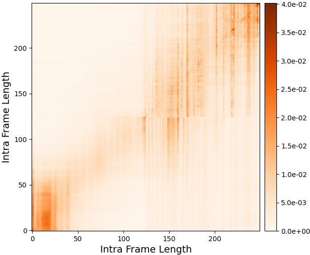
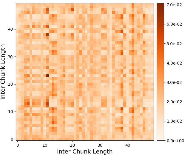
(IntraCA , InterCA )
4 Conclusion
In this work, we propose Tiny-Sepformer, a tiny Transformer network for speech separation. The Convolution-Attention network splits the features to two paths, and replaces one path with light 1D separable convolution. We also shared the layer parameters within the CA block, to further reduce the model parameters. The proposed Tiny-Sepformer achieves comparable separation results, and has relatively small model size. In addition, we found that large convolution channels within the chunk and more attention channels among the chunks could further improve the performance. The analysis of attention matrix weights explain the reason for the choice of this channel division configuration. For future works, we are also interested in exploring better model structure for fast inference speed. Memory consumption and time cost are both crucial for real-world application, like streaming speech separation scenarios.
5 Acknowledgement
This paper is supported by the Key Research and Development Program of Guangdong Province under grant No.2021B0101400003. Corresponding author is Jianzong Wang from Ping An Technology (Shenzhen) Co., Ltd (jzwang@188.com).
References
- [1] J. Zhu, M. Hasegawa-Johnson, and L. Sari, “Identify speakers in cocktail parties with end-to-end attention,” in IEEE Conference of the International Speech Communication Association (INTERSPEECH), 2020, pp. 3092–3096.
- [2] J. Luo, J. Wang, N. Cheng, and J. Xiao, “Unidirectional memory-self-attention transducer for online speech recognition,” in IEEE International Conference on Acoustics Speech and Signal Processing Proceedings (ICASSP), 2021, pp. 910–914.
- [3] D. Petermann, G. Wichern, Z.-Q. Wang, and J. Le Roux, “The cocktail fork problem: Three-stem audio separation for real-world soundtracks,” in IEEE International Conference on Acoustics, Speech and Signal Processing (ICASSP). IEEE, 2022, pp. 526–530.
- [4] X. Zhang, J. Qian, Y. Yu, Y. Sun, and W. Li, “Singer identification using deep timbre feature learning with knn-net,” in 2021 IEEE International Conference on Acoustics, Speech and Signal Processing (ICASSP). IEEE, 2021, pp. 3380–3384.
- [5] Q. Wang, I. Moreno, M. Saglam, K. Wilson, A. Chiao, R. Liu, Y. He, W. Li, J. Pelecanos, M. Nika, and A. Gruenstein, “Voicefilter-lite: Streaming targeted voice separation for on-device speech recognition,” in IEEE Conference of the International Speech Communication Association (INTERSPEECH), 2020, pp. 2677–2681.
- [6] X. Zhang, J. Wang, N. Cheng, and J. Xiao, “Singer identification for metaverse with timbral and middle-level perceptual features,” in International Joint Conference on Neural Networks, (IJCNN). IEEE, 2022, pp. 1–7.
- [7] E. Tzinis, S. Venkataramani, Z. Wang, C. Subakan, and P. Smaragdis, “Two-step sound source separation: Training on learned latent targets,” in IEEE International Conference on Acoustics, Speech and Signal Processing (ICASSP), 2020, pp. 31–35.
- [8] S. Chen, Y. Wu, Z. Chen, J. Wu, J. Li, T. Yoshioka, C. Wang, S. Liu, and M. Zhou, “Continuous speech separation with conformer,” in IEEE International Conference on Acoustics, Speech and Signal Processing (ICASSP), 2021, pp. 5749–5753.
- [9] Y. Luo and N. Mesgarani, “Tasnet: time-domain audio separation network for real-time, single-channel speech separation,” in IEEE International Conference on Acoustics, Speech and Signal Processing (ICASSP), 2018, pp. 696–700.
- [10] Y. Luo, N. Mesgarani, and Z. Chen, “Conv-tasnet: Surpassing ideal time-frequency magnitude masking for speech separation,” IEEE Transactions on Audio, Speech, and Language Processing (TASLP), vol. 27, no. 8, pp. 1256–1266, 2019.
- [11] J. Luo, J. Wang, N. Cheng, G. Jiang, and J. Xiao, “Multi-quartznet: Multi-resolution convolution for speech recognition with multi-layer feature fusion,” in IEEE Spoken Language Technology Workshop (SLT), 2021, pp. 82–88.
- [12] J. Luo, J. Wang, N. Cheng, E. Xiao, J. Xiao, G. Kucsko, P. O’Neill, J. Balam, S. Deng, A. Flores, B. Ginsburg, J. Huang, O. Kuchaiev, V. Lavrukhin, and J. Li, “Cross-language transfer learning and domain adaptation for end-to-end automatic speech recognition,” in IEEE International Conference on Multimedia and Expo (ICME), 2021, pp. 1–6.
- [13] Y. Luo, Z. Chen, and T. Yoshioka, “Dual-path rnn: Efficient long sequence modeling for time-domain single-channel speech separation,” in IEEE International Conference on Acoustics, Speech and Signal Processing (ICASSP), 2020, pp. 46–50.
- [14] J. Chen, Q. Mao, and D. Liu, “Dual-path transformer network: Direct context-aware modeling for end-to-end monaural speech separation,” in IEEE Conference of the International Speech Communication Association (INTERSPEECH), 2020, pp. 46–50.
- [15] C. Subakan, M. Ravanelli, S. Cornell, M. Bronzi, and J. Zhong, “Attention is all you need in speech separation,” in IEEE International Conference on Acoustics, Speech and Signal Processing (ICASSP), 2021, pp. 21–25.
- [16] S. Wang, B. Li, M. Khabsa, H. Fang, and H. Ma, “Linformer: Self-attention with linear complexity,” in IEEE Advances in Neural Information Processing Systems (NIPS), 2020.
- [17] K. Choromanski, V. Likhosherstov, D. Dohan, X. Song, A. Gane, T. Sarlos, P. Hawkins, J. Davis, A. Mohiuddin, L. Kaiser, D. Belanger, L. Colwell, and A. Weller, “Rethinking attention with performers,” in IEEE International Conference on Learning Representations (ICLR), 2021.
- [18] Y. Koizumi, S. Karita, S. Wisdom, H. Erdogan, J. Hershey, L. Jones, and M. Bacchiani, “Df-conformer: Integrated architecture of conv-tasnet and conformer using linear complexity self-attention for speech enhancement,” in IEEE Workshop on Applications of Signal Processing to Audio and Acoustics (WASPAA), 2021, pp. 161–165.
- [19] A. Gulati, J. Qin, C.-C. Chiu, N. Parmar, Y. Zhang, J. Yu, W. Han, S. Wang, Z. Zhang, Y. Wu, and R. Pang, “Conformer: Convolution-augmented transformer for speech recognition,” in IEEE Conference of the International Speech Communication Association (INTERSPEECH), 2020, pp. 5036–5040.
- [20] Z. Wu, Z. Liu, J. Lin, Y. Lin, and S. Han, “Lite transformer with long-short range attention,” in IEEE International Conference on Learning Representations (ICLR), 2020.
- [21] A. Hannun, A. Lee, Q. Xu, and R. Collobert, “Sequence-to-sequence speech recognition with time-depth separable convolutions,” in IEEE Conference of the International Speech Communication Association (INTERSPEECH), 2019, pp. 3785–3789.
- [22] Z. Lan, M. Chen, S. Goodman, K. Gimpel, P. Sharma, R. Soricut, G. Research, and M. de Carvalho, “Albert: A lite bert for self-supervised learning of language representations,” in IEEE International Conference on Learning Representations (ICLR), 2020.
- [23] P.-H. Chi, P.-H. Chung, T.-H. Wu, C.-C. Hsieh, Y.-H. Chen, S.-W. Li, and H.-y. Lee, “Audio albert: A lite bert for self-supervised learning of audio representation,” in IEEE Spoken Language Technology Workshop (SLT), 2021, pp. 344–350.
- [24] D. Yu, M. Kolbæk, Z.-H. Tan, and J. Jensen, “Permutation invariant training of deep models for speaker-independent multi-talker speech separation,” in IEEE International Conference on Acoustics, Speech and Signal Processing (ICASSP), 2017, pp. 241–245.
- [25] M. Kolbæk, D. Yu, Z.-H. Tan, and J. Jensen, “Multi-talker speech separation and tracing with permutation invariant training of deep recurrent neural networks,” IEEE Transactions on Audio, Speech, and Language Processing (TASLP), vol. 25, no. 10, pp. 1901–1913, 2017.
- [26] J. Hershey, Z. Chen, J. Le Roux, and S. Watanabe, “Deep clustering: Discriminative embeddings for segmentation and separation,” in IEEE International Conference on Acoustics, Speech and Signal Processing (ICASSP), 2016, pp. 31–35.
- [27] M. Ravanelli, T. Parcollet, P. Plantinga, A. Rouhe, S. Cornell, L. Lugosch, C. Subakan, N. Dawalatabad, A. Heba, J. Zhong, J.-C. Chou, S.-L. Yeh, S.-W. Fu, C.-F. Liao, E. Rastorgueva, F. Grondin, W. Aris, H. Na, Y. Gao, R. D. Mori, and Y. Bengio, “Speechbrain: A general-purpose speech toolkit,” in arXiv preprint arXiv:2106.04624, 2021.
- [28] N. Zeghidour and D. Grangier, “Wavesplit: End-to-end speech separation by speaker clustering,” IEEE Transactions on Audio, Speech, and Language Processing (TASLP), vol. 29, pp. 2840–2849, 2021.
- [29] D. Kingma and J. Ba, “Adam: A method for stochastic optimization,” in IEEE International Conference on Learning Representations (ICLR), 2014.
- [30] P. Micikevicius, S. Narang, J. Alben, G. Diamos, E. Elsen, D. Garcia, B. Ginsburg, M. Houston, O. Kuchaev, G. Venkatesh, and H. Wu, “Mixed precision training,” in IEEE International Conference on Learning Representations (ICLR), 2018.
- [31] E. Vincent, R. Gribonval, and C. Févotte, “Performance measurement in blind audio source separation,” IEEE Transactions on Audio, Speech, and Language Processing (TASLP), vol. 14, no. 4, pp. 1462–1469, 2006.