To Ask or Not To Ask: Human-in-the-loop Contextual Bandits
with Applications in Robot-Assisted Feeding
Abstract
Robot-assisted bite acquisition involves picking up food items with varying shapes, compliance, sizes, and textures. Fully autonomous strategies may not generalize efficiently across this diversity. We propose leveraging feedback from the care recipient when encountering novel food items. However, frequent queries impose a workload on the user. We formulate human-in-the-loop bite acquisition within a contextual bandit framework and introduce LinUCB-QG, a method that selectively asks for help using a predictive model of querying workload based on query types and timings. This model is trained on data collected in an online study involving 14 participants with mobility limitations, 3 occupational therapists simulating physical limitations, and 89 participants without limitations. We demonstrate that our method better balances task performance and querying workload compared to autonomous and always-querying baselines and adjusts its querying behavior to account for higher workload in users with mobility limitations. We validate this through experiments in a simulated food dataset and a user study with 19 participants, including one with severe mobility limitations. Please check out our project website at: emprise.cs.cornell.edu/hilbiteacquisition/.
I INTRODUCTION
Feeding, an essential Activity of Daily Living (ADL) [1], is challenging for individuals with mobility limitations, often requiring caregiver support that may not be readily available. Approximately 1 million people in the U.S. cannot eat without assistance [2], so robotic systems could empower these individuals to feed themselves, promoting independence. Robot-assisted feeding comprises two key tasks [3]: bite acquisition [4, 5, 6, 7], the task of picking up food items, and bite transfer [\citeconsecutivegallenberger2019transfer, belkhale2022balancing], delivering them to the user’s mouth. Our work focuses on bite acquisition, aiming to learn policies that robustly acquire novel food items with diverse properties.
With over 40,000 unique food items in a typical grocery store [10], bite acquisition strategies must generalize well to novel food items. Current approaches formulate bite acquisition as a contextual bandit problem [\citeconsecutivegordon2020adaptive,gordon2021leveraging], using online learning techniques like LinUCB [11] to adapt to unseen food items. However, these methods may need many samples to learn the optimal action, which is problematic due to food fragility and potential user dissatisfaction from failures [12].
Our key insight is that we can leverage the care recipient’s presence to develop querying strategies that can adapt to novel foods, giving users a sense of agency. Under the assumption that the human can specify the robot’s acquisition action, we extend the contextual bandit formulation to include human-in-the-loop querying [13]. However, excessive querying may overwhelm users and reduce acceptance [14]. Thus, our key research question is: How do we balance imposing minimal querying workload on the user while achieving maximal bite acquisition success in a human-in-the-loop contextual bandit framework?
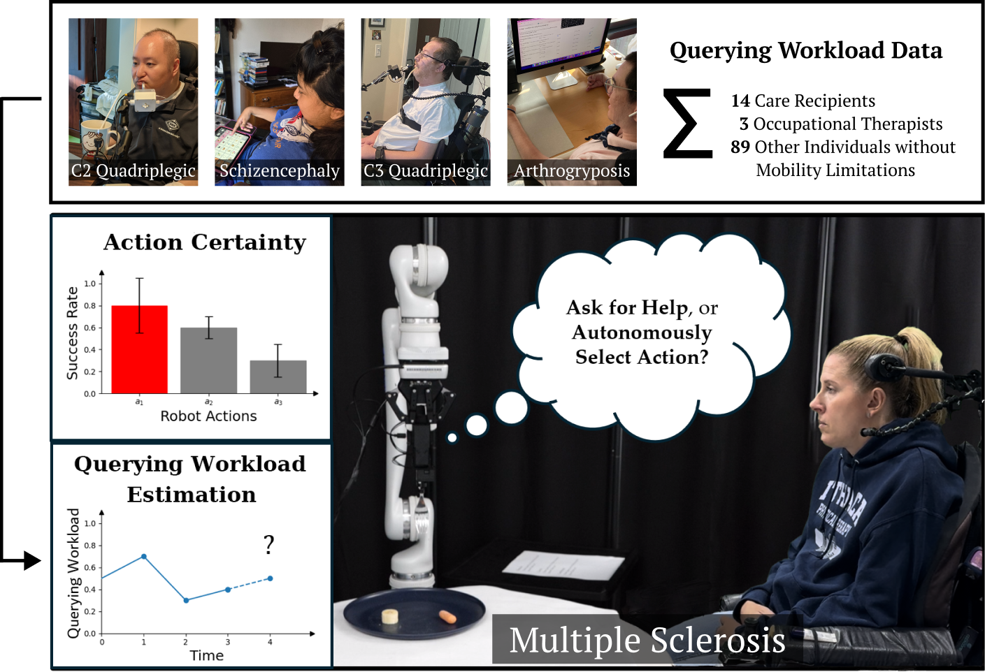
Balancing querying workload requires accurately estimating the workload imposed on users. Existing methods rely on physiological sensors [15, 16, 17], which can be invasive. We develop a non-intrusive, data-driven method by conducting a study on 14 participants with mobility limitations, 3 occupational therapists (OTs) who simulate the physical limitations of those with mobility limitations, and 89 participants without mobility limitations. We gather data on how different query types and timings impact self-reported workload using a modified NASA-TLX scale [18]. We tailor queries to common autonomous system failures, ranging from multiple-choice questions to open-ended prompts for acquisition strategy suggestions.
Using this data, we train a model to predict user workload in response to queries, considering the nature of the query and the user’s prior query interactions with the system. We observe statistically significant differences in self-reported workload between users with and without mobility limitations, which are accounted for by our learned models.
Building on our workload model, we propose LinUCB-QueryGap (LinUCB-QG), a novel algorithm for human-in-the-loop contextual bandits. It decides when to query based on the estimated querying workload and performance uncertainty of candidate actions. Simulated experiments on a dataset of 16 food items [4] show that LinUCB-QG is able to better balance workload and bite acquisition success compared to three baselines: (i) LinUCB [5], a state-of-the-art fully autonomous approach; (ii) AlwaysQuery, which always queries; and (iii) LinUCB-ExpDecay, a naive querying algorithm. LinUCB-QG achieves higher task performance than LinUCB and LinUCB-ExpDecay, with lower workload than AlwaysQuery. It also queries less when using a workload model trained on users with mobility limitations, indicating sensitivity to the workload differences across diverse user populations.
We validate our method in a real-world user study with 19 individuals, including one with Multiple Sclerosis, using three foods with variable material properties: banana slices, baby carrots, and cantaloupe. LinUCB-QG achieves a statistically significant 26% higher task success compared to LinUCB, and a 47% lower change in querying workload compared to AlwaysQuery.
Our contributions are as follows:
-
•
A human-in-the-loop contextual bandit framework incorporating querying workload for bite acquisition.
-
•
A dataset (including users with mobility limitations) on how feeding-related queries affect workload, and a predictive workload model without exteroceptive sensor inputs.
-
•
A novel method, LinUCB-QG, that balances acquisition success and querying frequency using our workload model, shown through simulations and a real-world study with 19 users, including one with severe mobility limitations.
II RELATED WORK
Human-in-the-loop algorithms. Our problem is an instance of learning to defer to an expert [19], where an agent decides whether to act autonomously or defer to experts like humans or oracle models. Most approaches operate in supervised learning [19, 20, 21, 22] or reinforcement learning domains [23]. Given the constraints of robot-assisted bite acquisition (observing independent contexts and receiving sparse feedback) we focus on learning-to-defer policies in an online contextual bandit setting. While prior methods often assume a fixed cost for querying the expert [20, 21, 22] or deal with imperfect experts [21], we propose estimating a time-varying deferral penalty using a data-driven model.
Other research explores active learning in robotics [24, 25, 26], where agents decide which instances to query [\citeconsecutiveracca2019teacher, li2023embodied] or which type of feedback to solicit [24]. Some algorithms balance task performance and human querying cost, but our work differs by using a data-driven model of querying cost and applying it to the complex task of bite acquisition.
Querying workload modeling. Our algorithms need to monitor workload to avoid over-querying users. For individuals with mobility limitations, querying workload may involve physical [27] and cognitive components [18], depending on the query type. Most workload estimation literature relies on neurological/physiological signals (ECG/heart rate, respiration [27], physical posture [28] for physical workload; EEG [15], EDA [29], pupil metrics [\citeconsecutiveahmad2019trust, fridman2018cognitive] for cognitive workload), training supervised models based on these signals. However, measuring such signals requires specialized, often invasive equipment. Alternatively, workload can be estimated post-hoc using subjective metrics like NASA-TLX [15].
In contrast, we develop a data-driven predictive model of querying workload using self-reported, modified NASA-TLX survey results, without relying on specialized sensors. Our model estimates the expected workload of a query based on interaction history, timing, and query type. Additionally, unlike prior work [\citeconsecutiveshayesteh2021investigating, fridman2018cognitive, rajavenkatanarayanan2020towards, ahmad2019trust], we focus on workload estimation for users with mobility limitations.
III PROBLEM FORMULATION
Following previous work [\citeconsecutivegordon2020adaptive, gordon2021leveraging], we formulate bite acquisition as a contextual bandit problem. At each timestep, the learner receives a context (food item), and selects actions that minimize regret over timesteps:
where is the reward, is the optimal action maximizing for , and expectations are over the stochasticity in . In our problem setting, we assume access to a dataset from a robotic manipulator, consisting of observations , actions , and rewards . This dataset is used to pretrain and validate our algorithms, but is not required for our online setting. Our contextual bandit setting is characterized by (more details in Appendix):
-
•
Observation space : RGB images of single bite-sized food items on a plate, sampled from 16 food types [4].
-
•
Action space : 7 actions in total: 6 robot actions shown in Fig. 2 (bottom) [\citeconsecutivebhattacharjee2019towards, feng2019robot], and 1 query action .
-
•
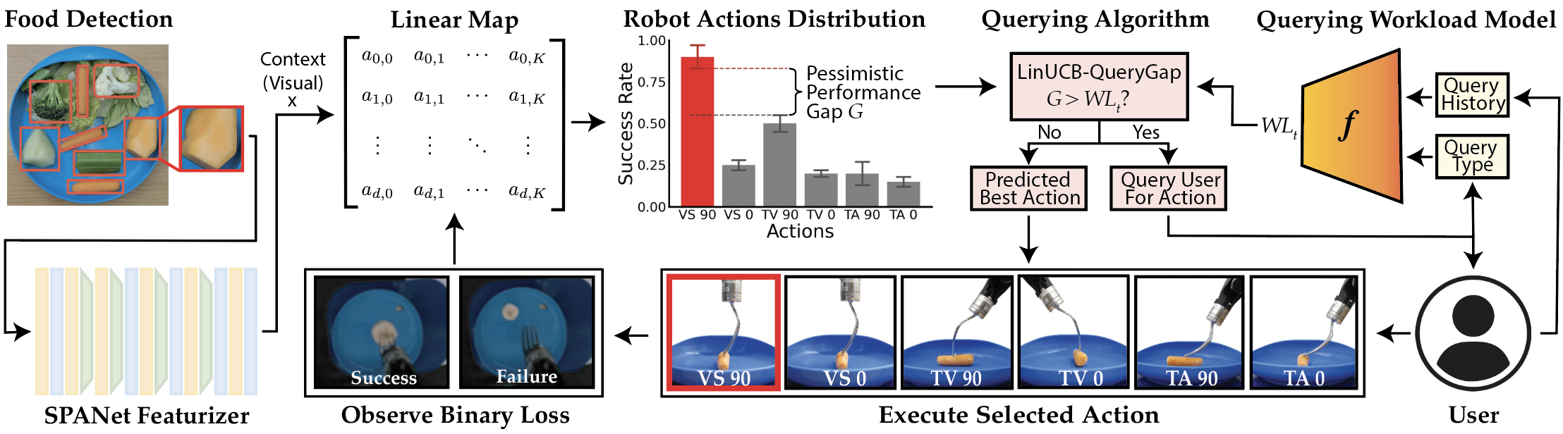
Context space : Lower-dimensional context derived from observations using SPANet [4], with dimensionality . As our bandit algorithms assume a linear relationship between and the expected reward , we use the penultimate activations of SPANet as our context since the final layer of SPANet is linear [5].
When the learner selects a robot action , it receives a binary reward indicating success for context . If the learner selects , it receives the optimal robot action from the human. It then executes that action and receives a reward. Querying imposes a penalty on the learner, given by the human’s latent querying workload state at time .
We model the total expected reward as the sum of the expected task reward (the probability that action succeeds for food context ) and the expected querying workload reward associated with selecting query actions :
where is a scalar weight in . We define to be if , and if , where is the probability that action succeeds for context . We define to be if , and if . Our goal is to learn a policy that maximizes .
IV querying workload Modeling
Our human-in-the-loop contextual bandit algorithms rely on estimating the querying workload state (Sec. III). To estimate , we first conduct a user study to understand how workload responds to queries (Sec. IV-A). We then learn a predictive workload model using this data (Sec. IV-C).
IV-A Querying Workload User Study
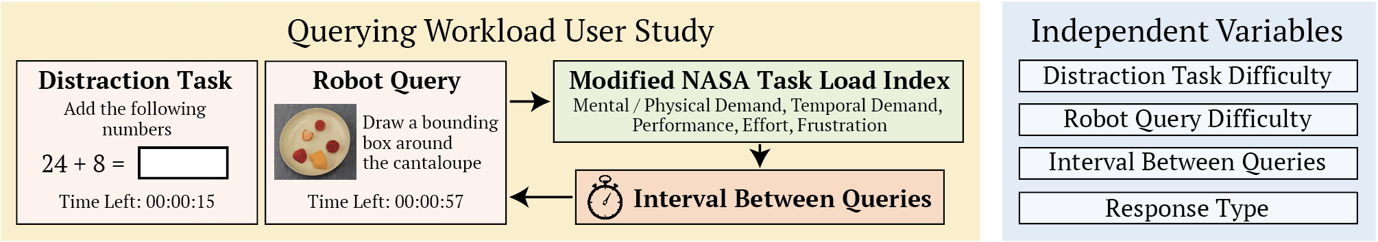
We design a user study (Fig. 3) to capture how different query types affect an individual’s querying workload in robotic caregiving scenarios. In such scenarios, a feeding system may request various assistance types from the user, such as semantic labels, bounding boxes for food items, or explanations for failed acquisition attempts. These response types can have varying impacts on workload [\citeconsecutivecui2021understanding, koppol2021interaction].
For instance, a semantic label response may impose less workload than an open-ended response. In addition, the end-user of the system and the caregiver may be busy with other tasks, such as watching TV while eating. We conduct an online user study that captures the above factors to determine how an individual’s querying workload changes in response to requests for assistance from an autonomous system.
Participants perform a distraction task while periodically receiving queries from a “robot,” simulating realistic caregiving situations where users might be engaged in other activities. The robot queries represent realistic assistance requests during bite acquisition. We vary four independent variables hypothesized to impact querying workload:
-
1.
Robot query difficulty (): 2 options – easy or hard.
-
2.
Distraction task difficulty (): 3 options – no distraction task, an easy numeric addition task, or a hard video transcription task.
-
3.
Time interval between queries (): 2 options – either 1 minute or 2 minutes.
-
4.
Response type (): 3 options – (a) a multiple-choice question (MCQ) asking for a semantic label, (b) asking the user to draw a bounding box (BB) around a food item, or (c) an open-ended (OE) question asking the user to explain why an acquisition attempt failed.
Each participant experiences 12 study conditions, one for each of the 2 settings of , 3 settings of , and 2 settings of , with the entire study taking roughly 1.5 hr. During each condition, lasting 5.5 minutes, participants engage in distraction tasks and respond to robot queries (with varying response types ) as shown in Fig. 3. We measure self-reported workload (our dependent variable) after each robot query and at the end of each condition using 5 modified NASA-TLX subscales [\citeconsecutivehart1988development, hertzum2021reference] (mental/physical, temporal, performance, effort, frustration), each measured on a 5-point Likert scale (see Appendix for exact question wording).
We collect data from 14 users (7 male, 7 female; ages 27-50) with mobility limitations resulting from a diverse range of medical conditions: spinal muscular atrophy (SMA), quadriplegia, arthrogryposis, cerebral palsy, Ullrich congenital muscular dystrophy, schizencephaly with spastic quadriplegia, spinal cord injury (including C2 and C3 quadriplegia). We additionally collect data from 3 occupational therapists (OTs), (3 female; ages 23-26), trained to simulate right/left hemiplegia (stroke). The OTs positioned one side of their body in full shoulder adduction, and elbow flexion to allow only 30 degrees of functional elbow joint range. Finally, we collect data from 89 users without mobility limitations (40 male, 49 female; ages 19-68). The population size for users with limitations is larger than the median () in studies of assistive robots [\citeconsecutivemankoff2010disability, nanavati2023physically].
IV-B Data Analysis
We consider three distinct datasets under which to train the workload model: , which only includes the data from the 89 users without mobility limitations; , which only includes the data from the 14 users with mobility limitations and 3 OTs; and , which includes both and . We convert the modified NASA-TLX responses into a single querying workload score by normalizing responses to 3 of the questions, and taking a weighted average (weight details in Appendix). We find a statistically significant difference in mean querying workload between () and (), as described in the Appendix.
IV-C Querying Workload Predictive Model
We develop a predictive model of querying workload based on the user study data (Sec. IV-A). Our models operate in discrete time, where the time variable refers to an integer number of timesteps since the beginning of a condition, where each timestep corresponds to a fixed time spacing (set to in our experiments). The model has the form , where is the initial workload, is the history of previous queries (where , , and are the query variables defined in Sec. IV-A), and are the model parameters.
Linear discrete-time models. To capture the dependency between the and , we use a linear predictive workload model inspired by Granger causality models [\citeconsecutivegranger1969investigating,liang2023randomization]:
where represents the effect of the query asked timesteps in the past on the workload at the current time , is the history length, and is a bias term. We train the model using linear regression, where we convert , , and into features using one-hot encodings, and generate a training pair for each robot task query in our study (see Appendix for more details about the Granger models).
Model selection. We train models , , and , corresponding to the datasets , , and , respectively (Sec. IV-B). 111When training these models, our assumptions about the time taken for users to complete the modified TLX surveys, particularly for users without mobility limitations, are in the Appendix.. The models and indicate models learned for the simulation experiments and the real-world user study, respectively. For our simulation experiments, we learn 3 separate models , , and (details in the Appendix). For our real-world user study, we only use 2 of the 3 real models: for the users without limitations and for the users with limitations. In our setting, and are models chosen based on cross-validation median test MSE on and , respectively (full model selection details in Appendix). We also train a model (cross-validation score: ), which has a higher mean and standard deviation MSE than (cross-validation score: ). This suggests that training only on leads to a higher-variance, less accurate model, compared to training on . Thus, it is still helpful to consider the data from users without limitations () when training our workload models.
V Human-in-the-Loop Algorithms
We develop decision-making algorithms that decide whether to ask for help or act autonomously, using the learned workload models in Sec. IV-C. Specifically, we consider four human-in-the-loop contextual bandit algorithms: one fully autonomous, and three that can query the human.
Fully autonomous algorithm. Our fully autonomous baseline is LinUCB [11], the state-of-the-art for acquiring unseen bite-sized food items like banana and apple slices [\citeconsecutivegordon2020adaptive, gordon2021leveraging]. LinUCB selects the action that maximizes a reward upper-confidence bound (UCB) estimate for each robot action, given by . Here, is the linear parameter vector learned through regression on contexts and observed rewards for actions , where includes contexts seen for during pretraining and online validation. The term corresponds to a confidence level, and is the UCB bonus with regularization strength . The size of reflects the reward estimate uncertainty for the given context-action pair.
Querying algorithms. The querying algorithms decide to query the human or select the action that maximizes .
-
1.
AlwaysQuery: always queries the user. 222For a particular food context , we assume that the user provides the optimal action when queried. However, the expert action may sometimes fail due to inherent action uncertainty (e.g. due to food property variability). Thus, if initially fails, AlwaysQuery will repeatedly execute until success.
-
2.
LinUCB-ExpDecay: queries with exponentially-decaying probability (decay rate ) depending on number of food items seen in an episode (see Appendix).
-
3.
LinUCB-Query-Gap (LinUCB-QG), defined in Algorithm 1: queries if the worst-case performance gap between the best action and second-best action exceeds the predicted workload, with scaling factor .
| Workload Model | |||
| –LinUCB | - | ||
| –AlwaysQuery | |||
| –LinUCB-ExpDecay | |||
| –LinUCB-QG | |||
| Workload Model | |||
| –LinUCB | - | ||
| –AlwaysQuery | |||
| –LinUCB-ExpDecay | |||
| –LinUCB-QG | |||
| Workload Model | |||
| –LinUCB | - | ||
| –AlwaysQuery | |||
| –LinUCB-ExpDecay | |||
| –LinUCB-QG |
In LinUCB-QG, the worst-case gap is the difference between a pessimistic estimate of ’s reward and an optimistic estimate of ’s reward, considering their confidence intervals (Fig. 2, top). A larger gap indicates a higher risk that the predicted best arm may be suboptimal, increasing the odds that the benefit of querying outweighs the workload penalty . Therefore, querying only when the gap is sufficiently large helps balance task reward and workload.
We define the predicted workload penalty to be the counterfactual workload if we were to query at the current time. To estimate this, we condition our workload model on the specific query type that we consider in our experiments. We use , where we set the query type variables to be , , “no distraction task” for all where the selected action .
VI EXPERIMENTS
We evaluate our human-in-the-loop algorithm performance using two setups: (i) a simulation testbed (Sec. VI-A), and (ii) a real world user study with 19 subjects (Sec. VI-B). We evaluate our algorithms on a surrogate objective, adapted from (Sec. III) (details in Appendix):
VI-A Simulated Testbed
We simulate food interaction using a dataset of bite-sized food items on plates, including 16 food types [4], each with 30 trials for the 6 robot actions . We first draw a random image of a given food type from the dataset and generate the corresponding context using SPANet. When the policy selects a robot action , we sample a binary task reward from a Bernoulli distribution with success probability . If , we declare that the bandit has converged, and move to a new food type at the next timestep. If , we draw a new random image of the same food type from the dataset until we exceed the maximum number of attempts . When the policy selects a query action , the bandit policy repeatedly executes the optimal action until convergence, or the limit is reached.
Metrics. We compute 5 objective metrics to evaluate the tradeoff between task performance and querying workload:
-
•
The mean task reward , measuring the efficiency of successful food acquisition.
-
•
The episodic change in workload .
-
•
Our surrogate objective , where represents a user-specific preference for the task performance/workload tradeoff.
-
•
The number of timesteps taken to converge , which provides additional insights into task performance.
-
•
The fraction of food items for which we queried , which provides an insight into querying workload.
Evaluating querying workload in simulation. In our simulation environment, we use the learned workload model for both LinUCB-QG action-selection, as well as computing the evaluation metrics and . During the rollout of a particular bandit policy, we evolve the workload model state according to the learned model when we query. We consider the three dataset scenarios and corresponding workload models , , and (Sec. IV-C), and set (a median initial workload).
Pretrain, validation, and test sets. In our experiments, we partition the set of 16 food types into a pretraining set (for the contextual bandit and for training SPANet), a validation set (for tuning the querying algorithm hyperparameters), and a test set (for metric evaluation). Our validation set (cantaloupe, grape) and test set (banana, carrot) include food items with varying material properties. Our pretraining set includes the remaining 12 food types in the food dataset. We use the validation set to select the hyperparameter that maximizes the weighted metric given a setting.
Results. We investigate how LinUCB-QG balances the tradeoff between task reward and querying workload. Table I compares the four algorithms for a setting with a slight preference for maximizing task performance over minimizing workload (). Across all three workload data settings, LinUCB-QG has a higher mean task reward than LinUCB and LinUCB-ExpDecay, and a mean weighted metric that is better than or competitive with the other methods (within the uncertainty of the simulation), suggesting that it achieves the best overall tradeoff between task reward and querying workload. Additionally, the querying fraction for LinUCB-QG increases from to to , suggesting that LinUCB-QG is sensitive to the higher workload predictions with care recipient and OT data, while still trading off task reward and workload.
Experiment: generalization on . We run an additional experiment to ablate , where at test time we use either or in LinUCB-QG action-selection, but use for metric evaluation (). We find that is lower in the first setting () compared to the second setting (), suggesting that including is crucial to achieve the best trade-off between task reward and workload for users with mobility limitations. See Appendix for more details and comparison metrics.
VI-B Real-World User Study
To evaluate the real-world performance-workload tradeoff of LinUCB-QG, we conduct a user study with 19 users: 18 users without mobility limitations (8 male, 10 female; ages 19-31; 66% with prior robot interaction experience), and one 46-year old user with Multiple Sclerosis since they were 19. We investigate whether LinUCB-QG improves task performance compared to LinUCB, while minimizing workload compared to Always-Query. This study was approved by the IRB at Cornell University (Protocol #IRB0010477).
Study setup. We use a Kinova Gen-3 6-DoF robot arm with a custom feeding tool (details in Appendix). For each method, we present users with a plate of 3 food items (banana, carrot, cantaloupe), with diverse characteristics: cantaloupe works with all robot actions; carrots require sufficient penetration force and fork tines perpendicular to the food major axis; bananas are soft, requiring tilted-angled actions [5]. We set for a reasonable study duration. The user provides feedback using a speech-to-text interface when queried, without any additional distraction tasks. Users evaluate each of the three methods in a counterbalanced order. We measure workload before/after each method by asking 5 modified NASA-TLX subscale questions: mental/physical, temporal, performance, effort, and frustration (question wording in Appendix). We conduct 2 repetitions of the 3 food items for all 3 methods (18 total trials).
Metrics. We define 7 subjective and 3 objective metrics to compare the methods. 4 subjective metrics correspond to the modified post-method NASA-TLX questions: Post-Mental Workload, Post-Temporal Workload, Post-Performance, and Post-Effort Workload. The other 3 subjective metrics measure workload changes during each method: Delta-Mental Workload, Delta-Temporal Workload, and Delta-Querying Workload (the change in querying workload score, weighting function in Appendix). The 3 objective metrics are mean task reward per plate (), mean successes per plate (), and mean query timesteps per plate ().
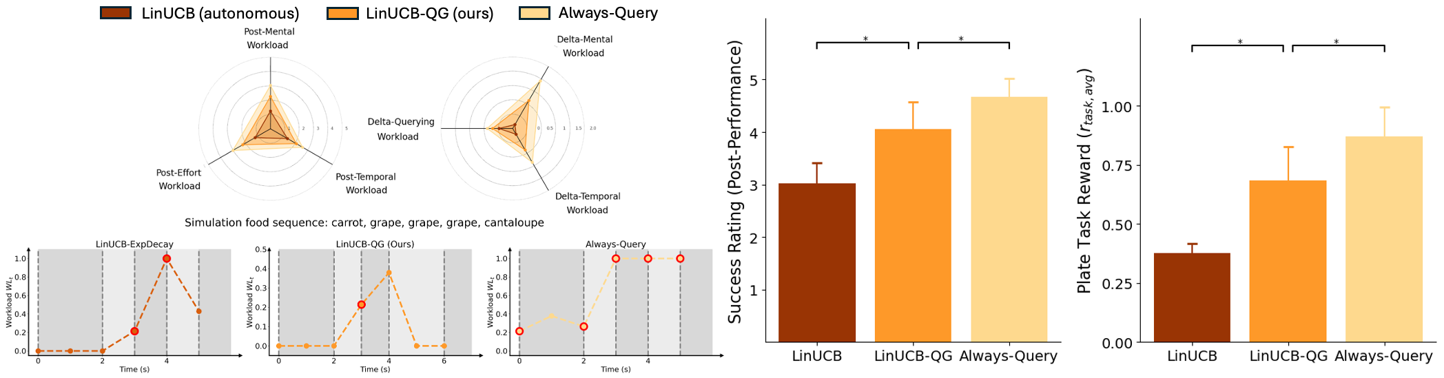
Overall results. Among the three methods, LinUCB-QG offers the most balanced approach to human-in-the-loop bite acquisition. It is more efficient than LinUCB and imposes less querying workload than Always-Query. While LinUCB typically picks up the carrot or cantaloupe within 1-2 timesteps but struggles with the banana, Always-Query successfully picks up food in the first timestep by always querying the user, leading to higher workload. Our method, LinUCB-QG, selectively asks for help with the banana and acts autonomously for the other foods in most trials, balancing task performance with querying workload.
(1) Task success results: Fig. 4 (right) shows that LinUCB-QG achieves higher objective () and subjective (Post-Performance) success ratings versus LinUCB, our autonomous baseline, showing greater efficiency. (2) Querying workload results: As shown in Fig. 4 (left, top), LinUCB-QG has lower subjective querying workload scores (mental, temporal, effort) compared to Always-Query, indicating that selective querying reduces workload. This is the case for both the post-method metrics (Post) and the workload change metrics (Delta). All results are statistically significant (Wilcoxon paired signed-rank test, ). See Appendix for full comparisons across all metrics.
Results: user with mobility limitations. We highlight observations from the user with mobility limitations. First, they provided a higher mean subjective success rating for LinUCB-QG than for LinUCB, aligning with the aggregate results. However, the user provided consistently low physical/mental, temporal and effort ratings across all methods. Potential reasons for this include the relative simplicity of providing feedback in our setting, and the fact that this particular user frequently requests assistance in daily life, reducing their querying workload. The user also commented that relying on external physiological signals (such as EEG) to estimate workload would add stress (due to the additional hardware required), reinforcing the benefit of non-intrusive workload models for human-in-the-loop querying algorithms.
Discussion. Future work could incorporate different query types in the real-world study, beyond the best acquisition action, such as the other query types in our workload model. In our setting, task complexity depends on physical food properties such as compliance or shape. We did not explicitly focus on such variables when modeling workload, although query difficulty does correlate with task complexity. The NASA-TLX scale has known limitations, such as subjectivity [38], over-emphasizing task difficulty [39], and workload score calculation problems [\citeconsecutivevirtanen2022weight, bolton2023mathematical], meaning that the modified NASA-TLX scores used to train our workload models are inherently noisy. We mitigate this by focusing on relative workload changes when evaluating how well our algorithms balance performance and workload. Additionally, we do not take measurements between queries in our workload dataset, so our workload models interpolate between queries using their learned weights, leading to rollouts that are not always intuitive (e.g. due to assigning greater weight to past queries). Future directions include predictive modeling with objective, non-intrusive workload measurements, and extensions to other assistive tasks where performance must be balanced with workload, using domain-agnostic workload features.
References
- [1] Sidney Katz et al. “Studies of illness in the aged: the index of ADL: a standardized measure of biological and psychosocial function” In jama 185.12 American Medical Association, 1963, pp. 914–919
- [2] Matthew W Brault “Americans with disabilities: 2010” In Current population reports 7, 2012, pp. 70–131
- [3] Rishabh Madan et al. “Sparcs: Structuring physically assistive robotics for caregiving with stakeholders-in-the-loop” In 2022 IEEE/RSJ International Conference on Intelligent Robots and Systems (IROS), 2022, pp. 641–648 IEEE
- [4] Ryan Feng et al. “Robot-assisted feeding: Generalizing skewering strategies across food items on a plate” In The International Symposium of Robotics Research, 2019, pp. 427–442 Springer
- [5] Ethan K Gordon et al. “Adaptive robot-assisted feeding: An online learning framework for acquiring previously unseen food items” In 2020 IEEE/RSJ International Conference on Intelligent Robots and Systems (IROS), 2020, pp. 9659–9666 IEEE
- [6] Ethan K Gordon et al. “Leveraging post hoc context for faster learning in bandit settings with applications in robot-assisted feeding” In 2021 IEEE International Conference on Robotics and Automation (ICRA), 2021, pp. 10528–10535 IEEE
- [7] Priya Sundaresan, Suneel Belkhale and Dorsa Sadigh “Learning visuo-haptic skewering strategies for robot-assisted feeding” In 6th Annual Conference on Robot Learning, 2022
- [8] Daniel Gallenberger, Tapomayukh Bhattacharjee, Youngsun Kim and Siddhartha S Srinivasa “Transfer depends on acquisition: Analyzing manipulation strategies for robotic feeding” In 2019 14th ACM/IEEE International Conference on Human-Robot Interaction (HRI), 2019, pp. 267–276 IEEE
- [9] Suneel Belkhale et al. “Balancing efficiency and comfort in robot-assisted bite transfer” In 2022 International Conference on Robotics and Automation (ICRA), 2022, pp. 4757–4763 IEEE
- [10] Alessandra Malito “Grocery stores carry 40,000 more items than they did in the 1990s” In MarketWatch, June 17, 2017
- [11] Lihong Li, Wei Chu, John Langford and Robert E Schapire “A contextual-bandit approach to personalized news article recommendation” In Proceedings of the 19th international conference on World wide web, 2010, pp. 661–670
- [12] Tapomayukh Bhattacharjee et al. “Is more autonomy always better? exploring preferences of users with mobility impairments in robot-assisted feeding” In Proceedings of the 2020 ACM/IEEE international conference on human-robot interaction, 2020, pp. 181–190
- [13] Yuchen Cui et al. “Understanding the relationship between interactions and outcomes in human-in-the-loop machine learning” In International Joint Conference on Artificial Intelligence, 2021
- [14] Terrence Fong, Charles Thorpe and Charles Baur “Robot, asker of questions” In Robotics and Autonomous systems 42.3-4 Elsevier, 2003, pp. 235–243
- [15] Shayan Shayesteh and Houtan Jebelli “Investigating the impact of construction robots autonomy level on workers’ cognitive load” In Canadian Society of Civil Engineering Annual Conference, 2021, pp. 255–267 Springer
- [16] Ayca Aygun et al. “Investigating Methods for Cognitive Workload Estimation for Assistive Robots” In Sensors, 2022
- [17] Lex Fridman, Bryan Reimer, Bruce Mehler and William T Freeman “Cognitive load estimation in the wild” In Proceedings of the 2018 chi conference on human factors in computing systems, 2018, pp. 1–9
- [18] Sandra G Hart and Lowell E Staveland “Development of NASA-TLX (Task Load Index): Results of empirical and theoretical research” In Advances in psychology 52 Elsevier, 1988, pp. 139–183
- [19] Maithra Raghu et al. “The algorithmic automation problem: Prediction, triage, and human effort” In arXiv preprint arXiv:1903.12220, 2019
- [20] Vijay Keswani, Matthew Lease and Krishnaram Kenthapadi “Towards unbiased and accurate deferral to multiple experts” In Proceedings of the 2021 AAAI/ACM Conference on AI, Ethics, and Society, 2021, pp. 154–165
- [21] Harikrishna Narasimhan et al. “Post-hoc estimators for learning to defer to an expert” In Advances in Neural Information Processing Systems 35, 2022, pp. 29292–29304
- [22] Hussein Mozannar and David Sontag “Consistent estimators for learning to defer to an expert” In International Conference on Machine Learning, 2020, pp. 7076–7087 PMLR
- [23] Shalmali Joshi, Sonali Parbhoo and Finale Doshi-Velez “Learning-to-defer for sequential medical decision-making under uncertainty” In arXiv preprint arXiv:2109.06312, 2021
- [24] Tesca Fitzgerald et al. “INQUIRE: INteractive querying for user-aware informative REasoning” In 6th Annual Conference on Robot Learning, 2022
- [25] Mattia Racca, Antti Oulasvirta and Ville Kyrki “Teacher-aware active robot learning” In 2019 14th ACM/IEEE International Conference on Human-Robot Interaction (HRI), 2019, pp. 335–343 IEEE
- [26] Amber Li and Tom Silver “Embodied Active Learning of Relational State Abstractions for Bilevel Planning” In arXiv preprint arXiv:2303.04912, 2023
- [27] Joshua Bhagat Smith, Prakash Baskaran and Julie A Adams “Decomposed physical workload estimation for human-robot teams” In 2022 IEEE 3rd International Conference on Human-Machine Systems (ICHMS), 2022, pp. 1–6 IEEE
- [28] Caroline E Harriott, Tao Zhang and Julie A Adams “Assessing physical workload for human–robot peer-based teams” In International Journal of Human-Computer Studies 71.7-8 Elsevier, 2013, pp. 821–837
- [29] Akilesh Rajavenkatanarayanan, Harish Ram Nambiappan, Maria Kyrarini and Fillia Makedon “Towards a real-time cognitive load assessment system for industrial human-robot cooperation” In 2020 29th IEEE International Conference on Robot and Human Interactive Communication (RO-MAN), 2020, pp. 698–705 IEEE
- [30] Muneeb Imtiaz Ahmad, Jasmin Bernotat, Katrin Lohan and Friederike Eyssel “Trust and cognitive load during human-robot interaction” In arXiv preprint arXiv:1909.05160, 2019
- [31] Tapomayukh Bhattacharjee, Gilwoo Lee, Hanjun Song and Siddhartha S Srinivasa “Towards robotic feeding: Role of haptics in fork-based food manipulation” In IEEE Robotics and Automation Letters 4.2 IEEE, 2019, pp. 1485–1492
- [32] Pallavi Koppol, Henny Admoni and Reid G Simmons “Interaction Considerations in Learning from Humans.” In IJCAI, 2021, pp. 283–291
- [33] Morten Hertzum “Reference values and subscale patterns for the task load index (TLX): a meta-analytic review” In Ergonomics 64.7 Taylor & Francis, 2021, pp. 869–878
- [34] Jennifer Mankoff, Gillian R Hayes and Devva Kasnitz “Disability studies as a source of critical inquiry for the field of assistive technology” In Proceedings of the 12th international ACM SIGACCESS conference on Computers and accessibility, 2010, pp. 3–10
- [35] Amal Nanavati, Vinitha Ranganeni and Maya Cakmak “Physically assistive robots: A systematic review of mobile and manipulator robots that physically assist people with disabilities” In Annual Review of Control, Robotics, and Autonomous Systems 7 Annual Reviews, 2023
- [36] Clive WJ Granger “Investigating causal relations by econometric models and cross-spectral methods” In Econometrica: journal of the Econometric Society JSTOR, 1969, pp. 424–438
- [37] Tengyuan Liang and Benjamin Recht “Randomization Inference When N Equals One” In arXiv preprint arXiv:2310.16989, 2023
- [38] Sandra G Hart “NASA-task load index (NASA-TLX); 20 years later” In Proceedings of the human factors and ergonomics society annual meeting 50.9, 2006, pp. 904–908 Sage publications Sage CA: Los Angeles, CA
- [39] Ryan D McKendrick and Erin Cherry “A deeper look at the NASA TLX and where it falls short” In Proceedings of the Human Factors and Ergonomics Society Annual Meeting 62.1, 2018, pp. 44–48 SAGE Publications Sage CA: Los Angeles, CA
- [40] Kai Virtanen, Heikki Mansikka, Helmiina Kontio and Don Harris “Weight watchers: NASA-TLX weights revisited” In TheoreTical issues in ergonomics science 23.6 Taylor & Francis, 2022, pp. 725–748
- [41] Matthew L Bolton, Elliot Biltekoff and Laura Humphrey “The mathematical meaninglessness of the NASA task load index: A level of measurement analysis” In IEEE Transactions on Human-Machine Systems 53.3 IEEE, 2023, pp. 590–599
- [42] Rajat Kumar Jenamani et al. “FLAIR: Feeding via Long-Horizon AcquIsition of Realistic dishes” Under submission to Robotics: Science and Systems (RSS) 2024.
- [43] Shilong Liu et al. “Grounding dino: Marrying dino with grounded pre-training for open-set object detection” In arXiv preprint arXiv:2303.05499, 2023
- [44] Alexander Kirillov et al. “Segment anything” In Proceedings of the IEEE/CVF International Conference on Computer Vision, 2023, pp. 4015–4026
APPENDIX
VI-C Problem Formulation
VI-C1 Details on Contextual Bandit Setting
Below we provide more details on the contextual bandit setting.
-
•
Observation space : In each RGB image, the food item is either isolated, close to the plate edge, or on top of another food item [4].
-
•
Action space : Each robot action is a pair consisting of one of three pitch configurations (tilted angled (TA), vertical skewer (VS), tilted vertical (TV)) and one of two roll configurations (, ), relative to the orientation of the food [\citeconsecutivebhattacharjee2019towards, feng2019robot].
-
•
Context space : SPANet, the network from which we derive our contexts , is pretrained in a fully-supervised manner to predict , the probability that action succeeds for observation .
VI-D Querying Workload User Study
VI-D1 NASA-TLX weighting function
Throughout the paper, we define the querying workload state to be the following weighted sum of the raw NASA-TLX subscales: .
VI-D2 Modified NASA-TLX Subscale Questions
Below are the question wordings that we use in our online workload user study, which are modified versions of the NASA-TLX subscales:
-
•
Mental/Physical Demand: “How mentally or physically demanding was the task?”
-
•
Temporal Demand: “How hurried or rushed was the pace of the task?”
-
•
Performance: “How successful were you in accomplishing what you were asked to do?”
-
•
Effort: “How hard did you have to work to accomplish your level of performance?”
-
•
Frustration: “How irritated, stressed, and annoyed were you?”
Note that for the users without mobility limitations, the wording of the Mental/Physical Demand task was the following: “How mentally demanding was the task?”. This is because we assumed that the physical demand to answer the workload questions was minimal for users without mobility limitations.
VI-D3 Baseline conditions
2 baseline conditions. Each baseline condition corresponds to a fixed setting of (either easy addition, or hard video transcription), without any robot query tasks.
VI-D4 Sample study questions
Below we provide examples of the robot queries that we ask in the online querying workload user study, covering each of the possible response types and question difficulties :
-
•
, : “What kind of food item is outlined in the image below?” (Responses: “Raspberry”, “Strawberry”, “Grape”, “Apple”, “I don’t know.”)
-
•
, : “Draw a box around only the strawberry.”
-
•
, : “Why did the Robot fail in acquiring the cantaloupe?”
-
•
, : “Which of the following images is tofu?” (Responses: “Left”, “Right”, “I don’t know”)
-
•
, : “Draw a box around only the carrot in the bottom right.”
-
•
, : “How would you skewer the following item with a fork?”
VI-D5 Compensation
Users without mobility limitations were compensated at a rate of $12/hr, for a total compensation of $18 for the entire study (as the study duration was 1.5 hr). The occupational therapists who simulated mobility limitations were compensated at a rate of $10/hr, for a total compensation of $15 for the entire study. The users with mobility limitations were compensated at a rate of $20/hr, for a total compensation of $30 for the entire study.
VI-D6 Mean querying workload difference, vs .
In Section IV-B, we describe finding a statistically significant difference in mean querying workload between (users without limitations) and (users with limitations and OTs), where had a mean querying workload of , and had a mean querying workload of . We run a Mann-Whitney U-test on the querying workload scores from and . The alternative hypothesis that we tested is that the distribution of workload values for is stochastically less than the distribution of workload values for . For this alternative hypothesis, we find that , indicating a statistically significant result for .
VI-E Querying Workload Predictive Model
VI-E1 Modified TLX survey timing information
When training the workload models, we make the following assumption about the amount of time taken for users to complete the modified TLX surveys. In the setting, we assume 0 seconds for the full user population (which only includes users without mobility limitations). In the setting, we assume 5 seconds for users without mobility limitations (and for two users in the population for whom we did not collect time data), and for the rest of the users with mobility limitations, we used the logged time taken to complete the surveys. Our justification for this design choice is that in the setting, we would like the assumed time for users without mobility limitations to be appropriately scaled compared to the logged times for users with limitations, who took non-zero times to complete the surveys.
VI-E2 Discrete-time Models
We consider different values of , with one memoryless Granger model (where ) and a set of Granger models with ranging from to . We chose the upper bound of to roughly correspond to the study condition length in Section IV-A. This is because we set each discrete time step to correspond to . We zero-pad the query variables if there are no queries in the discrete time window , or if we run out of history.
For each of these models, we also consider variants where we impose non-negativity constraints and/or ridge-regression penalties on the weights and . Specifically, we consider 4 different variants:
-
•
Granger: no nonnegativity or ridge-regression penalty
-
•
Granger-Nonnegative (Granger-N): nonnegativity constraint only
-
•
Granger-Ridge (Granger-R): ridge-regression penalty only
-
•
Granger-Ridge-Nonnegative (Granger-RN): non-negativity constraint and ridge-regression penalty
VI-E3 Continuous-time Models
We also consider a continuous-time setting, where represents the querying workload at time . In this setting, we consider one model (denoted as Exp-Impulse) that models the workload at the current time as composed of a series of impulses at the query times, with an exponential decay in workload in between the queries. The Exp-Impulse model is defined recursively as follows:
where is the previous timestep at which we queried, is the magnitude of the impulse, and is the workload decay rate.
VI-E4 Model Selection
For each of the three dataset settings (, , ), we perform 4-fold cross-validation to select a model from the above set of linear models. Dataset consists of unique question/workload pairs, while dataset consists of unique question/workload pairs. For tuning of the ridge regression regularization parameter , we perform 5-fold cross validation to select the optimal parameter value, with a logarithmic range from to .
Table II shows predictive MSE statistics on the held-out test splits, computed across the 4 folds, for the set of learned models. Note that we also considered a constant baseline (denoted Constant), whose predicted workload is , and an average baseline (denoted Average), whose predicted workload is the average value of in the training set.
Real-world user study models. We describe the two simulated workload models (, ) that are used for the real-world experiments in Section VI-B, along with the mobility limitation-only model that is described in Section IV-C. The model is a Granger model with , with a ridge-regression penalty on and , where the final selected ridge regression penalty was . The model is a Granger model with . The model is a Granger model with and a ridge-regression penalty on and , where the final selected ridge regression penalty was . The model achieves a cross-validation mean test MSE of on , while achieves a cross-validation mean test MSE of on the dataset.
We use these models because they are the models with the lowest median test MSE on each dataset. We initially considered using mean test MSE to select the best-performing model, but we discovered that the mean test MSE had a very large magnitude for certain models. This is because for the model settings that do not have weight constraints, linear regression would overfit to the training set and learn model parameters with large weight magnitudes. Because of this, we use the median test MSE to select the model. Note that while the models have differences in their mean test MSE, the standard deviations in test MSE for the models overlap because of the variance across folds.
Simulated models. We describe the three simulated workload models (, , ) that are used in the experiments in Section VI-A. For all three models, we use Granger models with , where we place the following constraints on the parameters during model training: , . Placing these additional constraints guarantees that the predicted change in workload associated with a query is non-negative.
| Model | Test MSE () | Test MSE (median) | Test MSE () | Test MSE (median) | Test MSE () | Test MSE (median) | |
| Constant | 0 | ||||||
| Average | 0 | ||||||
| Granger | 1 | ||||||
| 5 | |||||||
| 10 | |||||||
| 15 | |||||||
| 20 | |||||||
| 25 | |||||||
| 30 | |||||||
| Granger-N | 1 | ||||||
| 5 | |||||||
| 10 | |||||||
| 15 | |||||||
| 20 | |||||||
| 25 | |||||||
| 30 | |||||||
| Granger-R | 1 | ||||||
| 5 | |||||||
| 10 | |||||||
| 15 | |||||||
| 20 | |||||||
| 25 | |||||||
| 30 | |||||||
| Granger-RN | 1 | ||||||
| 5 | |||||||
| 10 | |||||||
| 15 | |||||||
| 20 | |||||||
| 25 | |||||||
| 30 | |||||||
| Exp-Impulse | - | ||||||
VI-F Human-in-the-Loop Algorithms
We provide the full algorithmic description for LinUCB-ExpDecay in Algorithm 2.
VI-G Experiments: Simulated Testbed
VI-G1 Surrogate Objective
Here we justify our choice of the surrogate objective outlined in Section VI. Recall that the expected reward defined in Section III depends explicitly on the querying workload for all times for which . However, measuring the intermediate workload values after every query would require administering a survey after each query, which is impractical in the real world. Therefore, in our experimental formulation in both simulation and in the real study, we will assume that we cannot observe the intermediate workload values. Instead, we will observe only the initial and final workload workload values, which are and , respectively.
VI-G2 Additional Results
First, we include a set of additional metrics for the experimental setting described in Section VI-A, which focus on the observed convergence for each food item. We define the following metrics: , which is the fraction of food items for which the algorithm was unable to converge; and , which is the fraction of food items for which the algorithm autonomously converged. We also show , the change in querying workload across an episode and , the number of timesteps required to converge to the optimal action. Table III shows these metrics for .
| Workload Model | ||||
| –LinUCB | ||||
| –AlwaysQuery | ||||
| –LinUCB-ExpDecay | ||||
| –LinUCB-QG | ||||
| Workload Model | ||||
| –LinUCB | ||||
| –AlwaysQuery | ||||
| –LinUCB-ExpDecay | ||||
| –LinUCB-QG | ||||
| Workload Model | ||||
| –LinUCB | ||||
| –AlwaysQuery | ||||
| –LinUCB-ExpDecay | ||||
| –LinUCB-QG |
Next, we include full results for multiple settings of and , for the same querying workload models used in Section VI-A, ranging from shown in Tables IV, V, and VI (excluding , whose results are shown in Table I). In the setting, we see that LinUCB-QG generally performs the best for intermediate values of (corresponding to an intermediate emphasis on minimizing workload), while Always-Query performs the best for higher values of (corresponding to a high emphasis on maximum task performance, which the Always-Query baseline achieves due to its lack of exploration compared to LinUCB-QG). In the and settings, LinUCB performs the best for lower values of (because it never asks for help), while Always-Query performs the best for higher values of (where task performance is more critical). Nevertheless, in all data settings and across different values, LinUCB-QG offers better mean compared to LinUCB and LinUCB-ExpDecay, and competitive compared to the other methods.
| Method | ||||
| 0.2 | LinUCB | |||
| AlwaysQuery | ||||
| LinUCB-ExpDecay | ||||
| LinUCB-QG | ||||
| 0.3 | LinUCB | |||
| AlwaysQuery | ||||
| LinUCB-ExpDecay | ||||
| LinUCB-QG | ||||
| 0.4 | LinUCB | |||
| AlwaysQuery | ||||
| LinUCB-ExpDecay | ||||
| LinUCB-QG | ||||
| 0.5 | LinUCB | |||
| AlwaysQuery | ||||
| LinUCB-ExpDecay | ||||
| LinUCB-QG | ||||
| 0.6 | LinUCB | |||
| AlwaysQuery | ||||
| LinUCB-ExpDecay | ||||
| LinUCB-QG | ||||
| 0.8 | LinUCB | |||
| AlwaysQuery | ||||
| LinUCB-ExpDecay | ||||
| LinUCB-QG | ||||
| 0.9 | LinUCB | |||
| AlwaysQuery | ||||
| LinUCB-ExpDecay | ||||
| LinUCB-QG |
VI-G3 Additional Details: generalization on .
In this experiment, the validation process is analogous to that for the previous simulation results, but on the test set, we use separate workload models for LinUCB-QG action-selection, and for computing the evaluation metrics and . We use either or for the action-selection workload model, while we fix the evaluation workload model to be , and refer to the two settings as -on- and -on-, respectively. Table VII shows the results for LinUCB-QG in each of the two settings.
| Metric | -on- | -on- |
As mentioned in Section VI-A, we find that the mean weighted metric is higher in the -on- than the -on- setting (and and are both lower).
VI-G4 Sample Workload Model Rollout
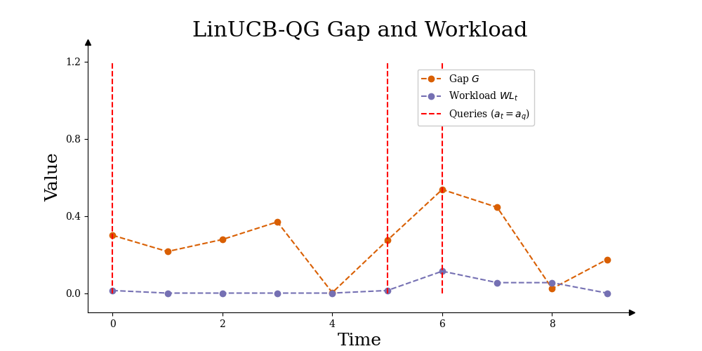
Finally, Figure 5 shows a rollout of the workload model in simulation for LinUCB-QG, showing how the workload evolves over time, how the UCB estimate gap variable varies, and when LinUCB-QG decides to query. In this example, LinUCB-QG decides to ask the human for help when (in this rollout, ), but also recall that once LinUCB-QG has asked for help for the current food item, it will continue to execute the expert action until it has converged.
VI-H Experiments: Real-world User Study
VI-H1 Feeding Tool
In our work, we use a custom feeding tool developed in prior work [\citeconsecutiverajatpriyarss2024, belkhale2022balancing], which is attached to the end of the Kinova’s Robotiq 2F-85 gripper. The tool consists of a motorized fork with two degrees of freedom: pitch and roll . Each of the six robot actions (for ) corresponds to a unique value of and . In particular, the pitch configuration (either TA, VS, or TV) affects the value of , while the roll configuration (either or ) affects the value of .
VI-H2 Details on Perception Modules
To more accurately determine skewering-relevant geometric information for each bite-sized food item, we leverage perception modules that were developed in prior work [42]. We use GroundingDINO [43] to produce an initial bounding box around the food item, followed by SAM [44] to segment the food item, and finally extract the minimum area rectangle around the segmentation mask to get a refined bounding box. From this bounding box, we derive the centroid and major axis of the food item, which are used by the low-level action executor to execute the desired robot action .
VI-H3 Additional Details and Analysis
Here we present additional details related to the real-world user study experiments outlined in Section VI-B.
Pre-method questions. We ask the users with mobility limitations the following questions prior to each method:
-
•
“How mentally/physically burdened do you feel currently?”
-
•
“How hurried or rushed do you feel currently?”
For users without mobility limitations, we ask the following questions:
-
•
“How mentally burdened do you feel currently?”
-
•
“How hurried or rushed do you feel currently?”
Post-method questions. We ask the users with mobility limitations the following questions after each method:
-
•
“For the last method, how mentally/physically burdened do you feel currently because of the robot querying you?”
-
•
“For the last method, how hurried or rushed do you feel currently because of the robot querying you?”
-
•
“For the last method, how hard did you have to work to make the robot pick up food items?”
-
•
“For the last method, how successful was the robot in picking up food items?”
For users without mobility limitations, we ask the following questions:
-
•
“For the last method, how mentally burdened do you feel currently because of the robot querying you?”
-
•
“For the last method, how hurried or rushed do you feel currently because of the robot querying you?”
-
•
“For the last method, how hard did you have to work to make the robot feed you?”
-
•
“For the last method, how successful was the robot in picking up the food item and bringing it to your mouth?”
Compensation. Users were compensated at a rate of $12/hr, for a total compensation of $18 for the entire study (as the study duration was 1.5 hr).
Note on initial workload . Although we do ask for an initial estimate of the user’s workload by asking the pre-method questions above, in our real-world experiments, we provide a fixed initial workload value of for LinUCB-QG. This value is used by LinUCB-QG for its internal workload predictions and decision-making. However, when calculating the subjective metrics in Section VI-B that measure changes in workload (Delta-Mental, Delta-Temporal, and Delta-Querying Workload), we use the responses to the pre-method questions to estimate the user’s initial workload.
Method comparison across all metrics. Tables VIII and IX include comparisons across the three methods used in the real-world user study (LinUCB, AlwaysQuery, LinUCB-QG) for the 7 subjective and 3 objective metrics mentioned in Section VI-B, respectively. For all metrics, we find that LinUCB-QG achieves an intermediate value for that metric compared to the other two algorithms, suggesting that our method finds a balance between querying workload and task performance (which these metrics cover). Additionally, Table X shows the full results of the Wilcoxon paired signed-rank tests that we used to determine whether LinUCB-QG exhibited statistically significant differences in the full set of metrics compared to LinUCB-QG and AlwaysQuery. For the metrics related to querying workload, our alternative hypothesis was that the value of the metric for LinUCB-QG was less than the value for AlwaysQuery. For the metrics related to task performance, our alternative hypothesis was that the value of the metric for LinUCB-QG was greater than the value for LinUCB. For all metrics, we find that LinUCB-QG has a statistically significant improvement compared to the baseline for that metric.
| Method | Post-Mental | Post-Temporal | Post-Performance | Post-Effort | Delta-Mental | Delta-Temporal | Delta-Querying Workload |
| LinUCB | |||||||
| AlwaysQuery | |||||||
| LinUCB-QG |
| Method | |||
| LinUCB | - | ||
| AlwaysQuery | |||
| LinUCB-QG |
| Metric | Hypothesis | |
| Post-Mental | LinUCB-QG AlwaysQuery | |
| Post-Temporal | ||
| Post-Effort | ||
| Delta-Mental | ||
| Delta-Temporal | ||
| Delta-Querying Workload | ||
| Post-Performance | LinUCB-QG LinUCB | |
Comments on Post-Performance metric. When looking at the Post-Performance metric, we find that LinUCB-QG achieves an intermediate value, higher than LinUCB but lower than Always-Query. When asking users to rate subjective success, we asked them to rate the overall success of each algorithm, which depends on both whether the algorithm successfully picked up food items and how many attempts were required for success. For this reason, we believe that users rated the success of Always-Query highly because it efficiently selects the optimal action for each food item within one timestep, whereas LinUCB-QG sometimes takes multiple timesteps if it does not query for a particular food item.
ACKNOWLEDGMENT
This work was partly funded by NSF CCF 2312774 and NSF OAC-2311521, a LinkedIn Research Award, and a gift from Wayfair, and by NSF IIS 2132846 and CAREER 2238792. Research reported in this publication was additionally supported by the Eunice Kennedy Shriver National Institute Of Child Health & Human Development of the National Institutes of Health and the Office of the Director of the National Institutes of Health under Award Number T32HD113301. The content is solely the responsibility of the authors and does not necessarily represent the official views of the National Institutes of Health.
The authors would like to thank Ethan Gordon for his assistance with the food dataset, Ziang Liu, Pranav Thakkar and Rishabh Madan for their help with running the robot user study, Janna Lin for providing the voice interface, Shuaixing Chen for helping with figure creation, Tom Silver for paper feedback, and all of the participants in our two user studies.