Topological Chaos in a Three-Dimensional Spherical Fluid Vortex
Abstract
In chaotic deterministic systems, seemingly stochastic behavior is generated by relatively simple, though hidden, organizing rules and structures. Prominent among the tools used to characterize this complexity in 1D and 2D systems are techniques which exploit the topology of dynamically invariant structures. However, the path to extending many such topological techniques to three dimensions is filled with roadblocks that prevent their application to a wider variety of physical systems. Here, we overcome these roadblocks and successfully analyze a realistic model of 3D fluid advection, by extending the homotopic lobe dynamics (HLD) technique, previously developed for 2D area-preserving dynamics, to 3D volume-preserving dynamics. We start with numerically-generated finite-time chaotic-scattering data for particles entrained in a spherical fluid vortex, and use this data to build a symbolic representation of the dynamics. We then use this symbolic representation to explain and predict the self-similar fractal structure of the scattering data, to compute bounds on the topological entropy, a fundamental measure of mixing, and to discover two different mixing mechanisms, which stretch 2D material surfaces and 1D material curves in distinct ways.
The essential allure of chaotic dynamics is confronting a complex, seemingly random, physical process and discovering the hidden, underlying patterns that order it. This is typified by the seminal experiments of Gollub and Swinney, showing that the progression from regular to turbulent fluid flow occurs via the predictable sequence of period doubling cascades.Gollub and Swinney (1975) Immense success has been achieved in unraveling such patterns for chaotic systems reducible to maps on a one- or two-dimensional phase spaceLi and Yorke (1975); Sharkovskii (1964); Milnor and Thurston (1988); Thurston (1988); Easton (1986). This has been achieved through a deep understanding of the shape of geometric objects living within the dynamical phase space, using topological tools such as Markov partitionsGuckenheimer and Holmes (1983), symbolic dynamicsLind and Marcus (1995); Kitchens (1998); Gilmore and Lefranc (2011), braid theoryBoyland, Aref, and Stremler (2000); Thiffeault and Finn (2006); Thiffeault (2010); Budišić and Thiffeault (2015); Stremler et al. (2011), and mapping class groups.Thurston (1988); Boyland (1994); Bestvina and Handel (1995) A key theme in such studies is topological forcing : the existence of certain short-time structures (e.g. low-period orbits) forces the existence of infinitely many longer-time structures. The resulting patterns are typically fractal, with symbolic rules describing a rich self-similarity. Thus, early-time, low-resolution data predicts long-time, high-resolution patterns. This is nicely illustrated by the famous period-three-implies-chaos result: the existence of a single period-three orbit of a map on the unit interval guarantees the existence of periodic orbits of arbitrary periodLi and Yorke (1975); Sharkovskii (1964). A central challenge in dynamical systems is extending these topological techniques to higher dimensions, for which there have been few clear paths forwardLefranc (2006); Lefranc, Morant, and Nizette (2008); Jung et al. (2010); Drótos et al. (2014); Drótos and Jung (2016). We demonstrate for the first time how chaotic scattering data for an explicit three-dimensional system, a numerical model of a chaotic time-periodic fluid vortex, reveals fractal rules of the dynamics.
Our results follow from developing a deep topological understanding of special 2D surfaces within the fluid; the stable and unstable manifoldsWiggins (1992) attached to stagnation points. These manifolds intersect an infinite number of times in a beautiful fractal pattern called a heteroclinic tangle (Fig. 1b). The topology of the tangle has profound implications for the system dynamics. Our technique shows how to extract this topological information and turn it into a symbolic representation of the dynamics. This representation captures the core mixing mechanism of the fluid, generates a lower bound on the (topological) entropy, and reveals distinct mechanisms for 1D and 2D material stretching. This work builds on the topological understanding of heteroclinic tangles in 2DEaston (1986, 1998); Rom-Kedar (1994); Rückerl and Jung (1994); Jung and Emmanouilidou (2005); Collins (1999, 2002, 2004), namely the homotopic lobe dynamics (HLD) techniqueMitchell et al. (2003); Mitchell and Delos (2006); Mitchell (2009, 2012); Sattari, Chen, and Mitchell (2016); Novick and Delos (2012); Byrd and Delos (2014), and a recent studyMaelfeyt, Smith, and Mitchell (2017) showing how HLD extends to 3D for certain tailor-made topological constructions, defined absent any explicit dynamics.
Successfully extending the 2D HLD technique to 3D paves the way for a structural characterization of the chaotic dynamics of other volume-preserving systems, like charged particles following magnetic field lines, shifting granular media, as well as many other 3D fluid flows. Furthermore, the HLD technique is algorithmic and amenable to automation. This would enable the analysis of much longer timescales, and also permit analyses of bifurcating mixing mechanisms. Finally, this current work is a spring-board to further extending the HLD technique to 4D symplectic maps derived from three-degree-of-freedom Hamiltonian systems, opening up many more applications, e.g. to chaotic atomic and molecular scattering.
Chaotic Spherical Vortex
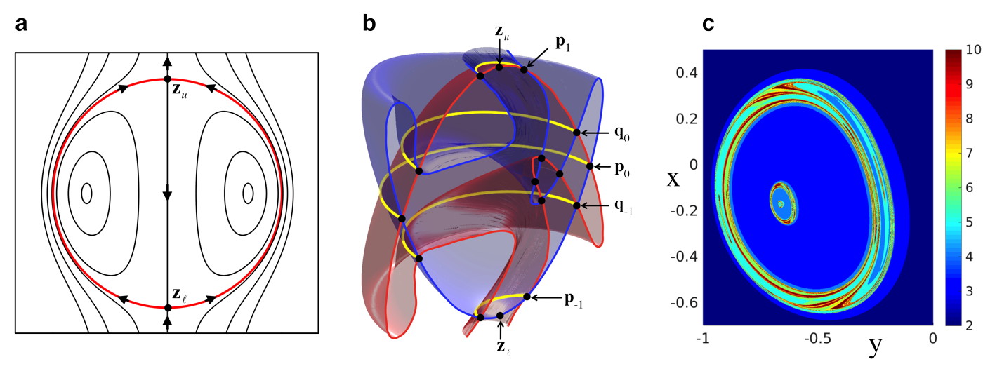
We analyze a numerically defined, physically representative, dynamical system that exists “in the wild” - passive advection in a modified Hill’s spherical vortex. Hill’s vortexHill (1894); Moffatt and Moore (1978) (see online methods) is a well known solution to Euler’s equations for an inviscid incompressible fluid (Fig. 1a). Two unstable stagnation points (fixed points), and , are connected by a 2D spherical separatrix, separating the vortex interior from its exterior. The separatrix prevents any mixing between fluid inside and outside the vortex.
To induce mixing and chaos, we modify Hill’s vortex by a sequence of time-periodic adjustments to the flow (see online methods). The resulting volume-preserving advection map, , which evolves an initial point forward for one period under the fluid flow to the final point , becomes our primary object of study. This advection map breaks rotational symmetry, but preserves both fixed points and reversibility.Strogatz (2014) (Reversing time is equivalent to reflecting about the -plane.) The separatrix splits into two distinct surfaces, the 2D unstable manifold of and the 2D stable manifold of (Fig. 1b). (The stable/unstable manifold consists of all points that converge upon / in forward/backward time.) These two manifolds first intersect at the primary intersection curve, , defining the unstable cap , the piece of the unstable manifold between and , and stable cap . The vortex interior is defined as the region between the stable and unstable caps. The stable and unstable manifolds are invariant: each point on the manifold maps forward to another point on the manifold. Thus, an intersection curve, e.g. , maps forward and backward to other intersection curves, e.g. and (Fig. 1b).
Escape-Time Plots and Reconstructing the Tangle
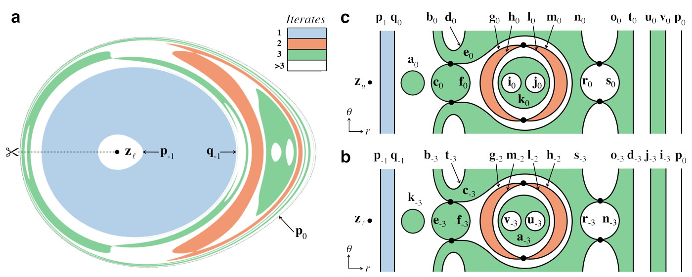
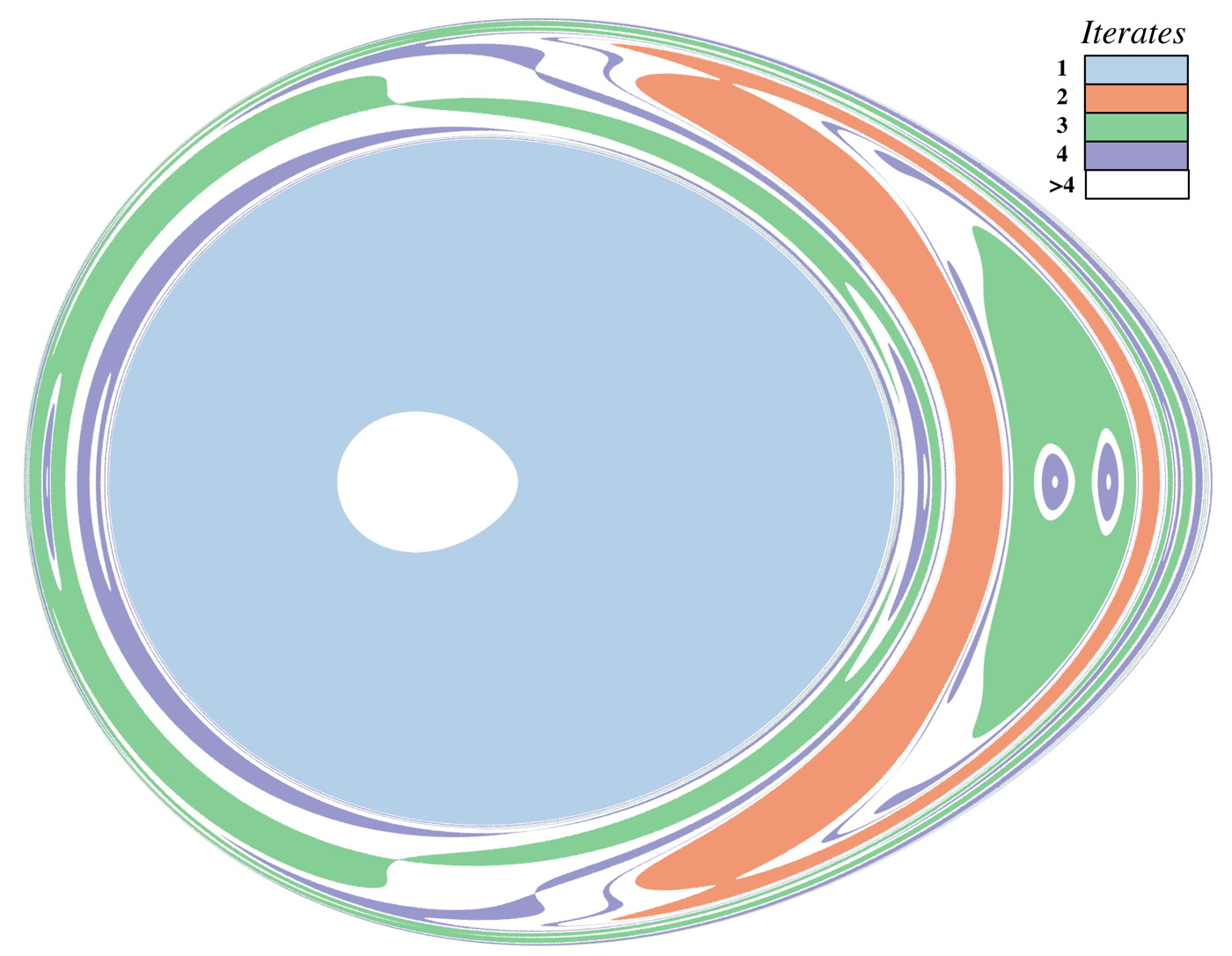
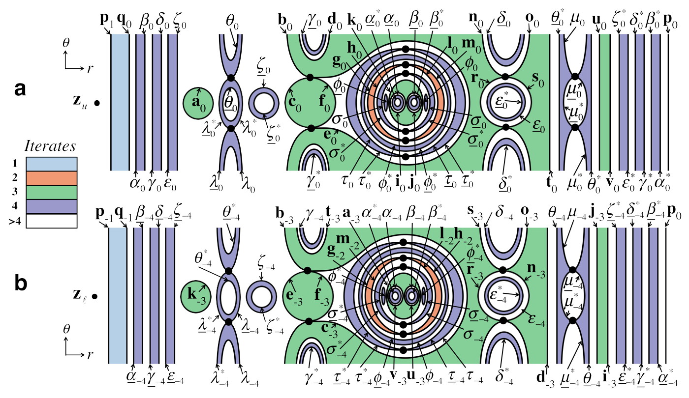
Due to the broken separatrix, some advected particles that originate outside the vortex will enter the vortex and subsequently escape. We treat this as a scattering problem. Fig. 1c shows the number of periods needed to pass from the plane below the vortex through the plane above the vortex. Note the intricate fractal structure as a function of the two impact parameters and . For our symbolic analysis, we shall use a scattering function that is easier to interpret. In Fig. 2a, the two impact parameters identify an initial point on the unstable cap, restricted to the fundamental unstable annulus between and . Escape is defined by leaving the vortex. (See online methods.) This defines the forward escape-time plot (ETP); the backward ETP is defined analogously for initial points in the fundamental stable annulus moving backward in time. Since the numerical ETP (Fig. 2a) includes difficult-to-see thin features, we provide clearer cartoons of the forward ETP (Fig. 2b) and backward ETP (Fig. 2c). We shall derive the symbolic dynamics from information in these ETPs up to iterate three.
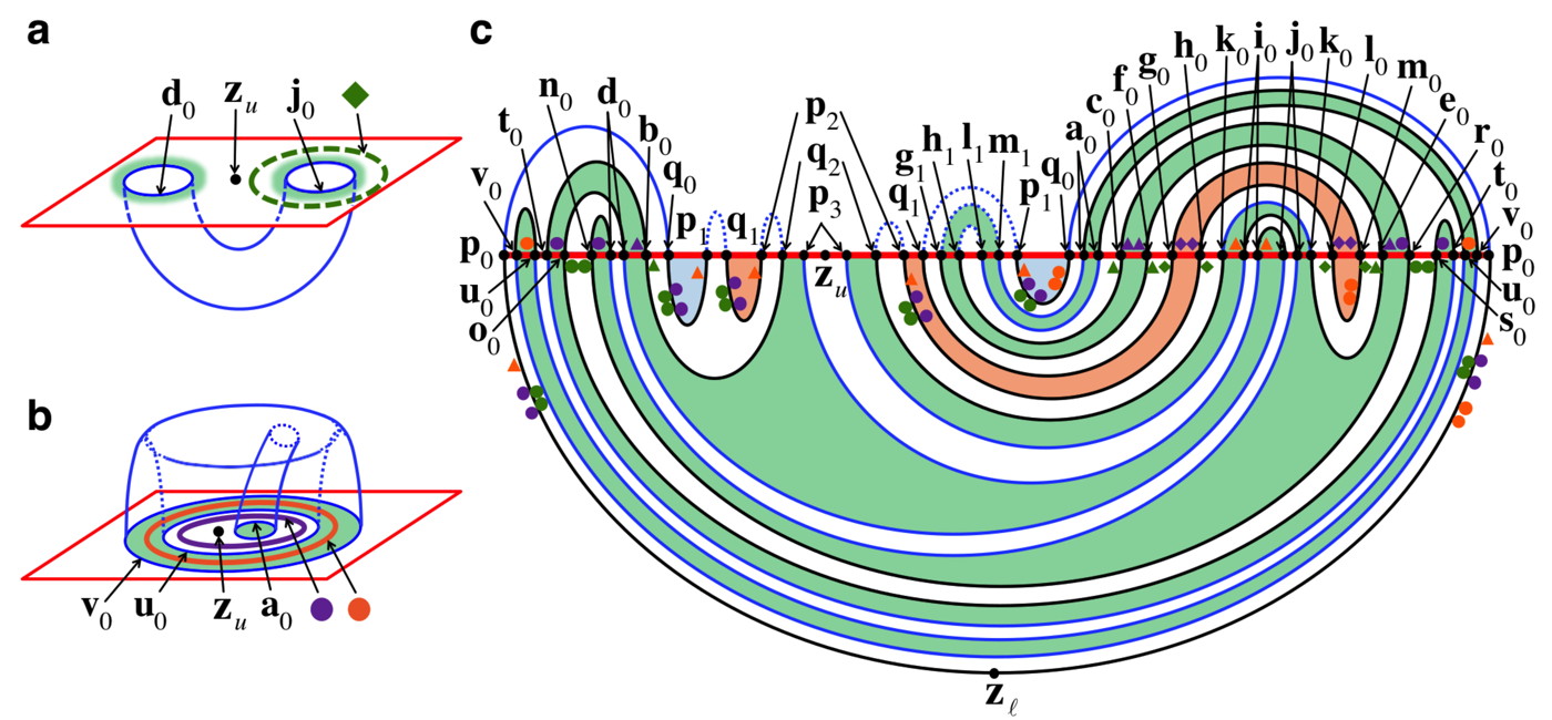
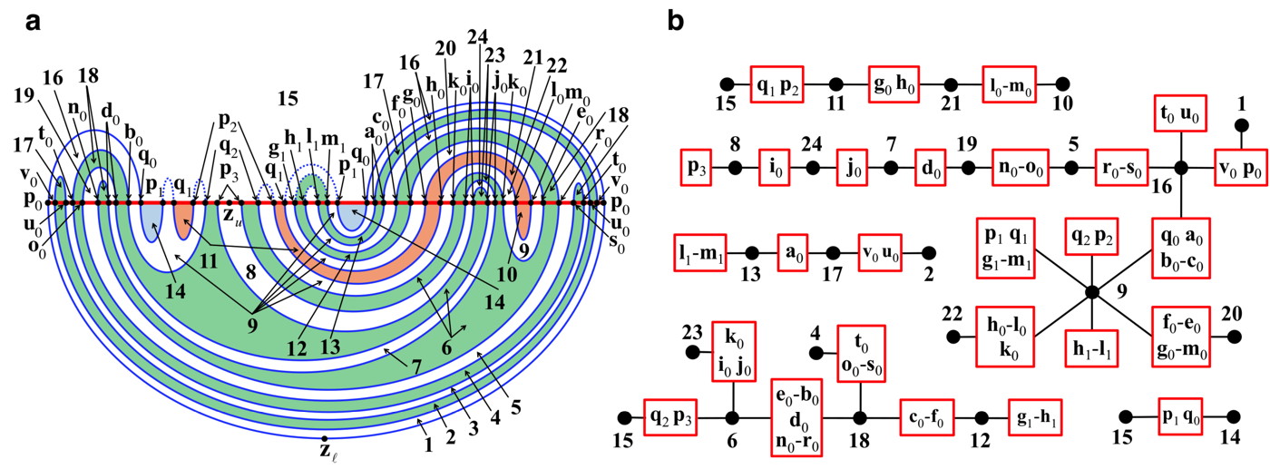
The unstable manifold is partitioned into pieces, called bridges, by cutting along the stable cap. Each bridge is identified by a labeled set of intersection curves on the stable cap, e.g. (Fig. 3a) or (Fig. 3b). The forward ETP contains escape domains, i.e. connected domains of constant escape time, which can be identified by their boundary labels, e.g. . Each escape domain eventually maps to a bridge outside the vortex, e.g. maps to . Similarly, each gap between escape domains, up to a given iterate, maps to an interior bridge, e.g. maps to . Thus, the boundaries of the escape domains are intersection curves between the stable and unstable manifolds. Furthermore, each boundary curve in Fig. 2b is paired with a curve in Fig. 2c to which it maps, e.g. maps to after three iterates.
To reconstruct a bridge from its boundaries, connect up each of its boundary curves with a 2D surface of genus zero (i.e. no “handles”) that doesn’t intersect the rest of the unstable manifold. (Stable/unstable manifolds cannot self-intersectWiggins (1992).) For example, the outer bridge (Fig. 3b) looks like the top of a bisected torus, where and form the concentric boundary circles, connected to a tube whose other boundary is . Similarly, the inner bridge (Fig. 3a) is a simple tube connecting to . The bridges fit inside one another like a convoluted set of nesting matryoshka dolls. To visualize this, Fig. 3c shows a cross-section of the tangle up to iterate three of the fundamental unstable annulus. While we develop our analysis of the perturbed Hill’s vortex using information up to iterate three, we have also completed this analysis up to iterate four, and include these results where applicable.
Enforcing Topology: Obstruction Rings and Bridge Classes
Now comes a crucial trick: we judiciously place obstruction rings within the 3D phase space. Bridges are now viewed as rubber sheets that can be arbitrarily distorted so long as they do not pass through the rings. A minimal set of rings is needed to enforce the tangle topology of Fig. 3c, preventing bridges from pulling through the stable cap and reducing the topological complexity. This set is constructed by placing rings near special intersections (see online methods). These rings are seen in profile in Fig. 3c. To appreciate the rings’ function, consider the outer bridge (Fig. 3b). The orange ring keeps the upper half torus connecting and from sliding down through the stable cap, while the purple ring plays the same role for the tube connecting to .
Obstruction rings partition the set of bridges into equivalence classes. Two bridges are of the same homotopy class, or bridge class, if one can be continuously deformed into the other without passing through a ring. These bridge classes form the central symbolic objects in our analysis, and their behavior under iteration constitutes a symbolic dynamical system.
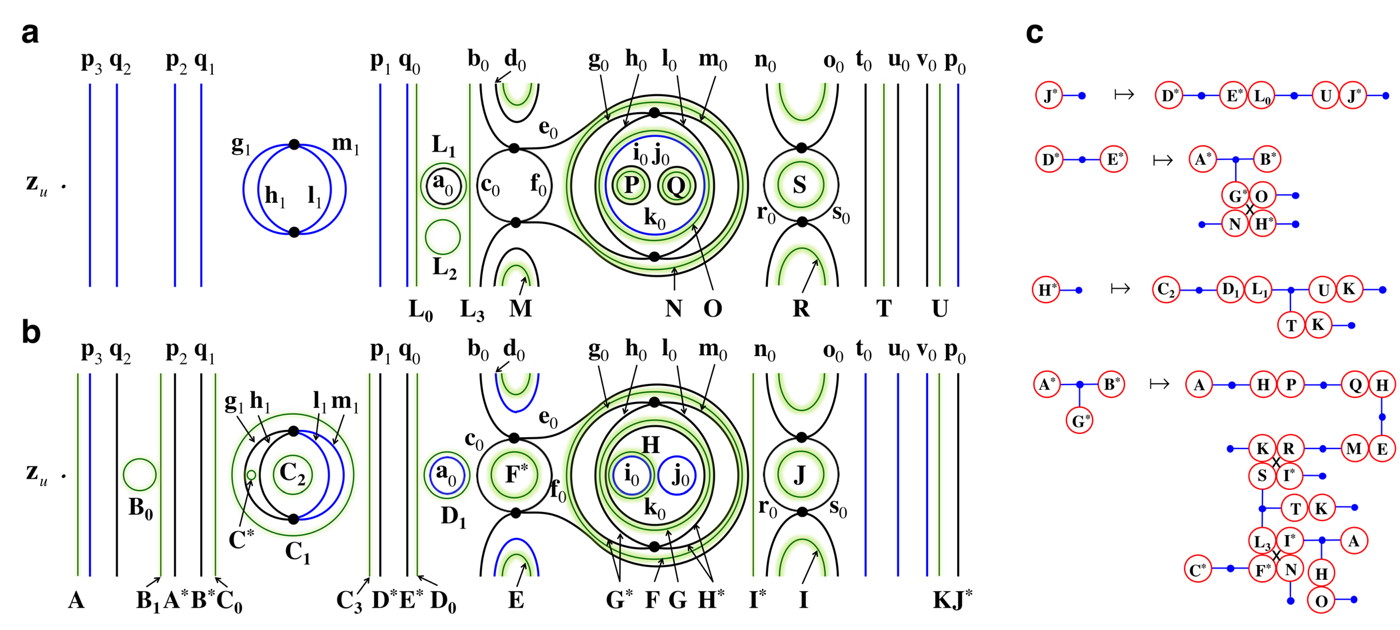
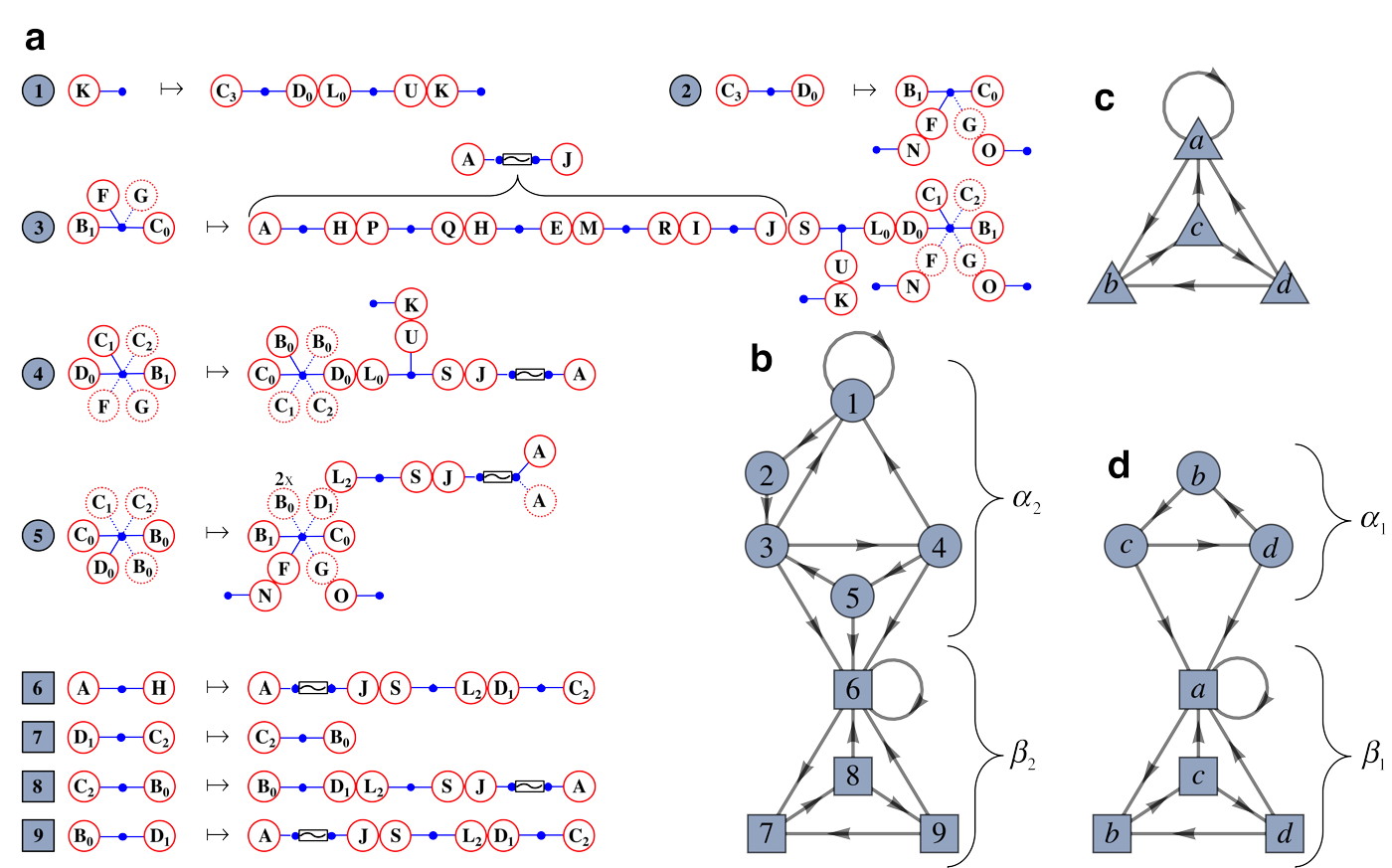
Just as bridges can be specified by their boundary curves, bridge classes can be specified by the homotopy classes, or boundary classes, of these curves. These boundary classes are defined as follows. The bridges with obstruction rings attached (black curves in Fig. 3c) divide the stable cap into distinct regions. The outer bridges define one division and the inner bridges another, as shown by the black curves in Figs. 4a and 4b. Two boundary curves are in the same boundary class if one can be deformed into the other without passing through the black curves. The green curves in Fig. 4 represent the inner and outer boundary classes needed to label the bridge classes. For example, the bridge class of the outer bridge is specified by the boundary classes , while the bridge class of is specified by . The “barbell” pictograms of Fig. 4c are useful graphical representations of bridge classes. The labeled red circles represent the boundary classes on the stable cap, and the blue lines connecting them represent the bridge class itself.
Dynamics of the Bridge Classes
Evolving forward one period, each bridge maps to a set of alternating inner and outer bridges, glued together at their common boundary curves. Crucially, this idea extends to bridge classes (see Fig. 4c). The left side shows the class, in barbell form, of every bridge in the tangle up to iterate two. The right side shows what each of these classes maps to, depicted as a gluing together of bridge classes. The right side of Fig. 4c contains new classes not present on the left. We must compute how these new classes map forward (see online methods). Repeating this procedure, we eventually obtain a set of bridge classes that is closed under iteration. Computing how bridge classes map forward is much of the “real work” of the HLD technique.
Some classes, e.g. , only occur once when repeatedly iterating the unstable fundamental annulus forward. These transient, or non-recurrent, classes convey no long-term topological information, and are ignored. Similarly, we ignore all inert classes, those that map to exactly one class under repeated iterations. For example, every outer bridge class is inert.
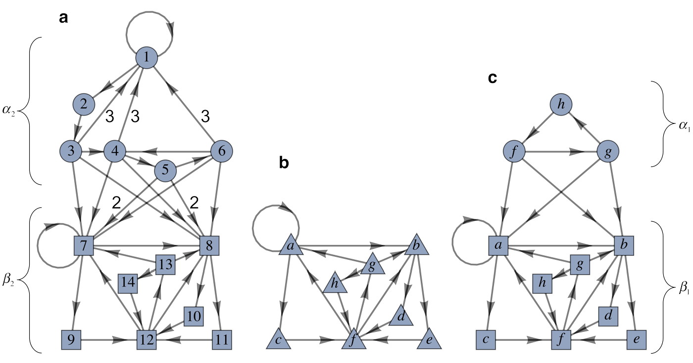
Figure 5a shows the remaining non-inert, or active, classes that are also recurrent, and their iterates. The graph in Fig. 5b records the allowed transitions between bridge classes: each vertex represents the correspondingly numbered class in Fig. 5a, and the directed edges show which classes are produced upon one iterate. The graph can also be presented as a transition matrix, , where is the number of directed edges connecting vertex to vertex .
The HLD analysis can be repeated for 1D bridges, paths beginning and ending on the stable cap and embedded in a 2D bridge. These 1D bridges can similarly be grouped into 1D bridge classes based on how they wrap around the obstruction rings. The forward iterates of 1D bridge classes can then be obtained by iterating forward the 2D bridge classes in which they are embedded. Fig. 5c shows the transition graph of the resulting symbolic dynamics.
Topological Entropy and Stretching Rates
The complexity of mixing in the vortex can be characterized by its topological entropy, which measures the exponential growth rate in the number of “distinguishable” orbits as a function of time Bowen (1971); Young (2003). Intimately related to this is the topological entropy of the symbolic dynamics, or symbolic entropy, which is computed as the log of the largest eigenvalue of the transition matrix. Since the symbolic dynamics represent the minimal topology forced by our knowledge of the tangle, its symbolic entropy is a strict lower bound to the full topological entropy of the advection map. Importantly, we can systematically increase this lower bound by including information about the tangle at successively higher iterates. For instance, our knowledge of the tangle up to iterate three (Fig. 5b) gives a symbolic entropy of , while the extra information gleaned at iterate four increases this to (see online methods). With increasing information about the tangle, the symbolic entropy will converge from below on the full topological entropy. We have directly computed this full topological entropy to lie between and using an independent approach Hunt and Ott (2015), thus confirming our symbolic calculation as a strict lower bound.
Topological entropy also measures the exponential stretching rate of the area or length of material advected in the fluid. The symbolic entropies of the graphs in Figs. 5b and 5c give lower bounds on the stretching rates of 2D material surfaces and 1D material lines, respectively. Differing 2D and 1D stretching rates is a unique possibility of the 3D HLD analysis, as seen in ref. Maelfeyt, Smith, and Mitchell (2017). However, in this example the 1D and 2D stretching rates are both for the iterate-three analysis and for the iterate-four analysis. Rather than being a coincidence, the equality of these two rates reflects a deeper structural similarity between the 1D and 2D stretching mechanisms, as discussed next.
Two Stretching Mechanisms
The transition graph (Fig. 5b) has two strongly connected components (SCCs), labeled and , i.e. subgraphs in which every vertex is reachable from every other vertex. Each SCC represents a distinct stretching mechanisms at work in the vortex. This distinction is revealed by a closer look at the dynamics of 1D bridge classes. Let () be the subset of 1D bridge classes that can be embedded in an () 2D bridge class. 1D bridge classes in Fig. 5c common to both and can be symbolically split to enable an “unfolded” version of the 1D symbolic dynamics graph, Fig. 5d. This splitting allows us to examine the stretching forced on 1D material lines by and separately.
Since Fig. 5c, (Fig. 5d), and (Fig. 5b) all show identical symbolic dynamics, the stretching of the 2D bridge classes is fundamentally 1D. Indeed, each bridge in the SCC is a simple tube, which stretches out along its axis to multiple such tubes under iteration, as can be seen in equations of Fig. 5a, where each barbell is mapped to a chain of barbells. On the other hand, since the dynamics of are trivial, i.e. have zero topological entropy, while those of are more complex, the stretching of bridge classes is irreducibly 2D in nature. As an example, consider the bridge class, labeled 1 in Fig. 5b, which is topologically an interior cap. While it is the central symbol in and participates in producing non-zero topological entropy, it does not force any 1D stretching, as any 1D bridge embedded in such a cap is contractible to a point. On the other hand, 2D bridges in are pushed down against the unstable cap and stretched out radially away from the lower fixed point. This fundamentally 2D behavior is also seen in equations of Fig. 5a, which exhibit branching not possible for 1D stretching. These two stretching mechanisms exist in the iterate-four dynamics as well. (See online methods).
While the two stretching mechanisms, and , are different in terms of the dimensionality of the structures which drive their stretching rates, their symbolic entropies are identical. More tellingly, when taken as formal symbolic dynamical systems, i.e. bi-infinite shifts of finite type, we discovered a strong shift equivalence between and , implying that their dynamics are identical up to topological conjugacyLind and Marcus (1995); Kitchens (1998). These facts holds at iterate-four as well. Far from being a coincidence, we conjecture that this equivalence is due to an underlying duality between forward-time 1D dynamics and backward-time 2D dynamics, and will appear in the dynamics forced by the tangle up to any iterate.
Fractal Structure
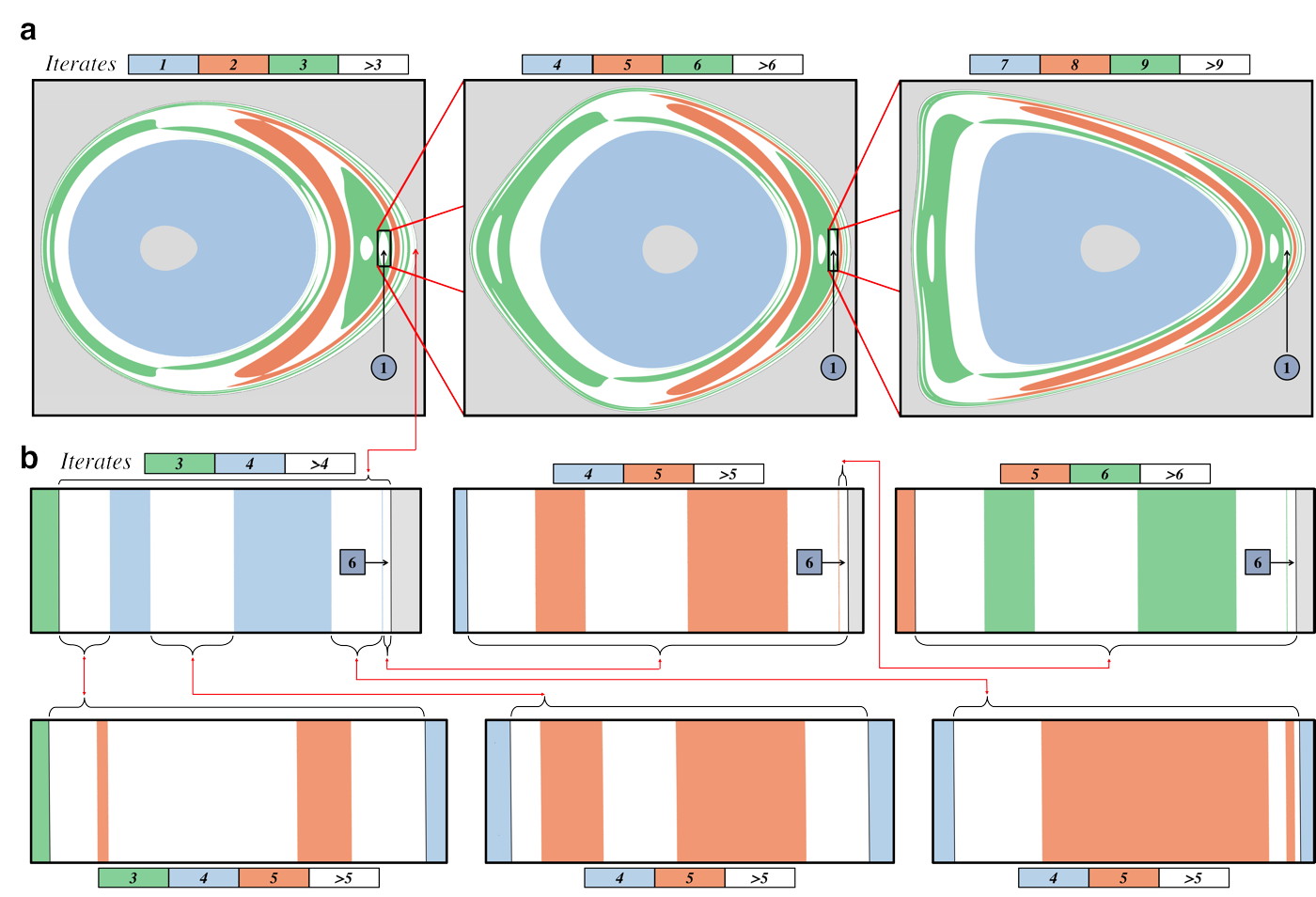
We started with scattering information in the ETPs, from which we derived a symbolic dynamics (Figs. 4c and 5a) for the minimal topological structure. This process can be reversed, and we can use the equations Fig. 4c and Fig. 5a, to fully reconstruct the ETPs. More importantly, we can predict new, topologically-forced, escape domains at higher iterates. These predictions provide a direct way to validate the symbolic dynamics by comparing them to numerical ETP results at higher iterates. Particularly interesting as test cases are cycles in the transition graph, which generate fractal self-similar patterns in the ETP. Each symbol represents a motif in the overall fractal, and every gap in the ETP that corresponds to this symbol will contain the same pattern at higher iterates. As an example, consider the 3-cycle in Fig. 5b, or more precisely, the analogous cycle in the iterate-four symbolic dynamics (see online methods). Every symbol “1” generated upon traversing this cycle once corresponds to a gap in each of the three panels of Fig. 6a. Zooming into this gap replicates this motif ad infinitum. Since this cycle is within the stretching mechanism, the associated motif is fundamentally 2D. Contrast this with the 1-cycle of 6 repeated within the stretching mechanism, whose associated fractal is shown in the top three boxes of Fig. 6b. This fractal structure is a zoomed-in portion of concentric annuli, which highlights its 1D nature. In both example fractals, the symbolic dynamics predict the exact fractal structure in the numerical ETPs. Note that iterate-four information was needed to produce such accurate symbolic dynamics, demonstrating the necessity —and power— of folding in new information at higher iterates. Indeed, at iterate five and higher, escape domains exist that are not predicted by iterate-four knowledge, e.g. the lower row of Fig. 6b shows extra, unpredicted bands at iterate five. Aside from being beautiful manifestations of the complexity inherent in the vortex, this fractal analysis reinforces the important idea that our finite knowledge of the scattering data has forced the existence of an infinite succession of predictable structures in the tangle.
Methods
Hill’s Spherical Vortex. This well known fluid flow is given by the stream-functionHill (1894); Moffatt and Moore (1978)
| (1) |
where are the radial and azimuthal spherical coordinates (no equatorial dependence), is the vortex radius (set to ), and is the magnitude of the uniform velocity field far from the vortex (set to ). Changing to cylindrical coordinates, the velocity field is and . This velocity field,
| (2) |
| (3) |
is volume preserving.
Modifications to the Fluid Flow. We first create a map, , by integrating initial points over the time interval , using the velocity field, Eq. (2) and (3). Next we compose with a series of maps, each intended to break a particular symmetry while maintaining certain features. To break the separatrix, we use the map, , where the strength of the perturbation is . To break the rotational symmetry about the z-axis, we apply a rotation about the y-axis, . The rotation angle, , is position dependent, , where . Finally, we introduce an additional rotation about the z-axis, , with , where . To ensure the final map is reversible, i.e. , where , we compose the functions as
This map is volume-preserving and also preserves the fixed points and .
Numerical Calculations. To numerically generate the stable and unstable caps, we start with linear approximations (small disks) of the stable and unstable manifolds near the two fixed points. These disks, represented by a high-density random sampling of points, are iterated (forward for and backward for ), until they intersect. These caps define the vortex boundary, and thereby enable us to build the escape-time plot (ETP).
The forward ETP begins as a small annulus on about the lower fixed point, , with a difference between its outer and inner radii large enough to capture a whole pre-iterate of the fundamental unstable annulus. Each of the randomly sampled points on this annulus are iterated forward until they have either exited the vortex, or reached a predetermined maximum number of iterates. We associate with each initial point the number of iterates it took to escape, i.e. its escape time. Next, we compute the Delaunay triangulation of these initial points. Escape domains are now identified as sets of points sharing a common escape time and all mutually connected through triangulation paths that contain only points in this set. The gaps are analogously identified for contiguous regions of points that have yet to escape at the maximum iterate. It should be noted that since escape domains are identified within gaps of smaller maximum iterate, gaps and escape domains form a natural tree structure which is convenient for data organization.
Domain boundaries are identified as triangles whose vertices do not share a common escape time. These triangles, and select adjacent triangles, can then be infilled with new points (which are themselves iterated forward) and re-triangulated to enable an iterative refinement of the boundaries. This allows us to increase the resolution of the forward ETP. Due to reversibility, the gaps and escape domains of the backward ETP are geometrically identical to those of the forward ETP. To create a complete backward ETP we must label each intersection curve as the forward iterate of a specific intersection curve in the forward ETP. To do this, we iterate every domain boundary in the forward/backward ETP forward/backward an appropriate number of times, and note which pairs coincide in phase space. Where this process was not possible, we used topological self-consistency to make the identification.
Heteroclinic Tangencies and Time-Reversal Symmetry. In addition to the transverse intersections between the stable and unstable manifolds that form closed curves, the dynamics also exhibit a countably infinite number of heteroclinic tangencies (the dots in the ETPs of Figs. 2b and 2c). At each of these sites, the two manifolds locally intersect like a flat plane intersecting a saddle, forming an “x” pattern. Thus, the intersection curves in each ETP are either simple closed curves, or collections of curve segments whose ends terminate at a tangency. Interestingly, the existence of reversibility ensures the robustness of these tangencies. Any perturbation to the unstable or stable manifold local to a tangency that removes this tangency necessarily violates reversibility. Thus, tangencies are robust under small changes to the parameter set , and are only removed through more global topological changes to the tangle.
Obstruction Rings and Pseudoneighbors. We algorithmically identify the set of obstructions rings, which enforce the given tangle topology and determine the equivalence relation defining the bridge classes, by first identifying specific intersection curves called pseudoneighbors. Pairs of intersection curves are pseudoneighbors if their iterates in the stable annulus can be connected by a path without crossing another intersection curve, and similarly for the unstable annulus. Every forward and backward iterate of a pseudoneighbor pair is likewise a pseudoneighbor pair. There is also the possibility of having a self-pseudoneighbor, a single intersection curve that bounds disks of and , that contain no other intersection curves. This definition of pseudoneighbors applies to intersection curves emanating from tangencies as well. Pseudoneighbors are essentially the minimal set of intersection curves whose existence force the existence of every other intersection curve up to a given iterate. The pseudoneighbors that lie in the stable annulus, seen in Fig. 2c, are , , , , and . The intersection curves separated by dashes indicate that they are connected through a heteroclinic tangency and should be considered as a single pseudoneighbor. Thus, the final three are self-pseudoneighbors associated with the three pairs of heteroclinic tangencies.
The obstruction rings are placed infinitesimally close to either intersection curve of a pseudoneighbor pair, perturbed away from the curve into the quadrant defined by the pieces of and connecting the pair of pseudoneighbors. Self-pseudoneighbors engender obstruction rings that are perturbed toward the interior of the region bounded by disks of and that have this self-pseudoneighbor as a mutual boundary. The obstruction rings associated with self-pseudoneighbors attached to tangencies are not rings, but copies of all the intersection curves mutually connected through tangencies, perturbed above and below the pseudoneighbor. Obstruction rings associated with pseudoneighbor pairs that lie on the stable cap outside of the stable annulus are not included, as they would serve to distinguish inert bridge classes that play no role in the active symbolic dynamics of Fig. 5b.
The Primary Division and Boundary Classes. Each bridge class is identified by its collection of boundary classes. In order to define boundary classes, we define an inner and outer division of the stable cap, which act as the equivalence-class-defining obstructions. These divisions are, in turn, restrictions of a division of the full 3D phase space, the primary division, to the stable cap. The primary division is constructed by dividing up phase space using the stable cap and every bridge that has an obstruction ring adjacent to it. The black lines in Fig. 3c show the primary division, while Figs. 4a and 4b show the inner and outer primary division that results, as well as the boundary classes. Each inner boundary class has a well defined boundary class as its forward iterate: , , , , , , , , , and .
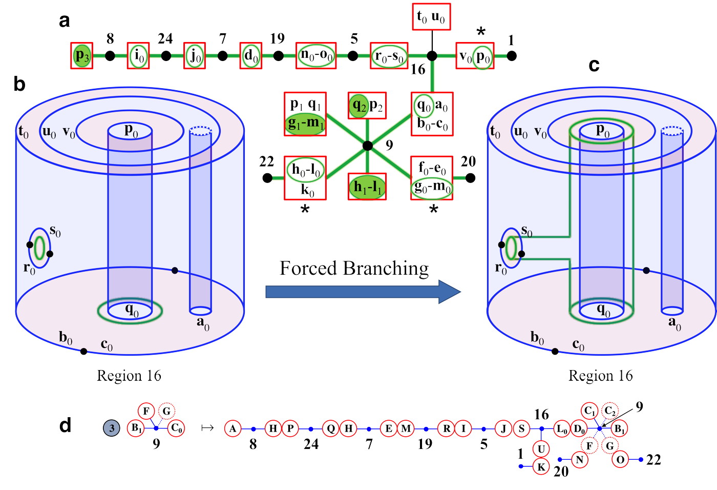
The Secondary Division. In order to algorithmically iterate bridge classes forward, particularly for bridges at iterates higher than the maximum iterate of the ETPs, we must first construct the secondary division of phase space. The secondary division is constructed by dividing phase space, as in Fig. 7a, along the forward iterate of each bridge that has a pseudoneighbor in its interior. The phase space regions that result from this division are numbered and their connections (at the stable fundamental annulus) are represented in the connection graphs of Fig. 7b. The forward iterate of each bridge class will be forced to extend through the appropriate connection graph, and conform to the topology of each numbered region.
Iterating Bridge Classes Forward. We can now take a bridge class and iterate all of its boundary classes forward. We must connect all of these boundary classes together, through the regions given in the connection graph, Fig. 7b, in the simplest way that is consistent with the topology of each region. This will in general force the existence of additional boundary classes in the forward iterate.
This forced connection can be done in a unique way, and results in a procedure for iterating any bridge class forward. At each node of a connection graph, representing a region of the secondary division, our task is to connect the boundary curves together in a way that doesn’t intersect any of the 2D unstable boundaries of this region, doesn’t include any “handles” which would change the genus of the overall topology of the unstable manifold, and forces the minimal number of new boundary curves. Figure 8 shows an example of this procedure. In each case of connecting boundary curves through a region, only the concise, minimal connecting surface is topologically unique. The actual unstable manifold might be more convoluted and topologically complex, which would be revealed by incorporating higher iterate information into our initial ETPs.
Inert Boundary Classes. The total set of bridge classes closed under iteration can be pruned, while preserving the essential symbolic dynamics, by removing non-recurrent and inert bridge classes. We can further reduce the size of the symbol set by introducing the concept of an inert boundary class, and treat any set of bridge classes whose constituents differ by only inert boundary classes as a single bridge class. An inert boundary class is defined by the effect its deletion has on the forward iterates of its parent bridge class. In particular, removing an inert boundary class does not modify the forward iterate of its parent bridge class other than to remove the forward iterate of this inert boundary class. Additionally, the forward iterate of an inert boundary class must itself be an inert boundary class. The base case which grounds this recursive definition is given when the bridge class replicates itself under iteration, and the inert boundary class iterates to itself. For example, the boundary class in the bridge class , represented by the symbol 3 in Fig. 5a, is inert (red dashed circle). The only effect deleting it would have would be to delete boundary class from the bridge class (symbol 4 and part of the forward iterate of 3). in is itself inert, as we can see by following its forward iterates; first in (symbol 5) and then in the bridge class (symbol 6 after removing the inert ). Note that a boundary class is not intrinsically inert, and can only be considered inert with respect to a specific bridge class. While in is inert, in (symbol 7) or (symbol 8) is not inert. Deleting from either of these would reduce their forward iterates in Fig. 5a to a single trivial cap.
4th Iterate ETP and Symbolic Dynamics. The analysis in the main text was done using ETP information up to third iterate. Shown in Fig. 9 and Fig. 10 is the ETP up to iterate four. Using the HLD analysis presented in the main text and elaborated upon in the online methods, the information embedded in this fourth iterate ETP results in the symbolic graphs of Fig. 11. The fourth iterate symbolic entropy associated with Fig. 11a is . Again, the graph has two strongly connected components (SCCs), labeled and , which correspond to a 2D and 1D stretching mechanism respectively.
Strong Shift Equivalence. As formal Markov shift dynamical systems, the symbolic dynamics embodied in the graphs of Figs. 5 and 11 can be analyzed using a powerful set of tools. In particular, two graphs can be considered conjugate, i.e. encoding essentially the same dynamics, if they can be connected by a chain of specific vertex merging and splitting operations.Lind and Marcus (1995); Kitchens (1998) This specific relation is also referred to as a strong shift equivalence (SSE). We have implemented an algorithm which searches for such a chain connecting two given transition matrices. First, for both transition matrices, we generate every matrix less than a given dimension that is reachable through no more than a given number of such merging and splitting moves. As this process unfolds, we periodically prune each set such that no two matrices are simply related by index permutations. We then compare the matrices in both accumulated sets. If there is a permutation-related pair, then the two original transition matrices are conjugate. If not, then we expand the length of allowable chains and repeat the procedure. While this algorithm can find an SSE, it cannot prove the absence of such an equivalence, as often the connecting chains of matrices are either quite long, or require that at least one of their members be a matrix of dimension much higher than the original transition matrices.
Determination of strong shift equivalence has allowed us to identify the duality between the forward time 2D stretching mechanism and the backward time 1D stretching mechanism. Additionally, the merging operation provides a convenient way of identifying bridge classes (vertices) that can be merged, and therefore should be considered equivalent. Indeed, this serves as an algorithmic way of checking for the existence of inert boundary classes, or whether unnecessary bridge classes were originally used (say due to superfluous obstruction rings).
References
References
- Gollub and Swinney (1975) J. P. Gollub and H. L. Swinney, “Onset of turbulence in a rotating fluid,” Phys. Rev. Lett. 35, 927–930 (1975).
- Li and Yorke (1975) T.-Y. Li and J. A. Yorke, “Period three implies chaos,” American mathematical monthly , 985–992 (1975).
- Sharkovskii (1964) A. N. Sharkovskii, “Co-existence of cycles of a continuous mapping of the line into itself,” Ukrainian Math. J. 16, 61–71 (1964).
- Milnor and Thurston (1988) J. Milnor and W. Thurston, “On iterated maps of the interval,” in Dynamical systems (College Park, MD, 1986–87), Lecture Notes in Math., Vol. 1342 (Springer, Berlin, 1988) pp. 465–563.
- Thurston (1988) W. P. Thurston, “On the geometry and dynamics of diffeomorphisms of surfaces,” Bull. Amer. Math. Soc. (N.S.) 19, 417–431 (1988).
- Easton (1986) R. W. Easton, “Trellises formed by stable and unstable manifolds in the plane,” Trans. Am. Math. Soc. 294, 719 (1986).
- Guckenheimer and Holmes (1983) J. Guckenheimer and P. Holmes, Nonlinear oscillations, dynamical systems, and bifurcations of vector fields (Springer, New York, 1983).
- Lind and Marcus (1995) D. Lind and B. Marcus, An introduction to symbolic dynamics and coding (Cambridge University Press, Cambridge, 1995) pp. xvi+495.
- Kitchens (1998) B. P. Kitchens, Symbolic dynamics, Universitext (Springer-Verlag, Berlin, 1998) pp. x+252, one-sided, two-sided and countable state Markov shifts.
- Gilmore and Lefranc (2011) R. Gilmore and M. Lefranc, The Topology of Chaos: Alice in Stretch and Squeezeland, 2nd ed. (Wiley-Interscience, 2011).
- Boyland, Aref, and Stremler (2000) P. L. Boyland, H. Aref, and M. A. Stremler, “Topological fluid mechanics of stirring,” J. Fluid Mech. 403, 277–304 (2000).
- Thiffeault and Finn (2006) J.-L. Thiffeault and M. D. Finn, “Topology, braids and mixing in fluids,” Phil. Trans. A 364, 3251 (2006).
- Thiffeault (2010) J.-L. Thiffeault, “Braids of entangled particle trajectories,” Chaos 20, 017516 (2010).
- Budišić and Thiffeault (2015) M. Budišić and J.-L. Thiffeault, “Finite-time braiding exponents,” Chaos 25, 087407 (2015).
- Stremler et al. (2011) M. A. Stremler, S. D. Ross, P. Grover, and P. Kumar, “Topological chaos and periodic braiding of almost-cyclic sets,” Phys. Rev. Lett. 106, 114101 (2011).
- Boyland (1994) P. Boyland, “Topological methods in surface dynamics,” Topol. Appl. 58, 223 (1994).
- Bestvina and Handel (1995) M. Bestvina and M. Handel, “Train-tracks for surface homeomorphisms,” Topology 34, 109 (1995).
- Lefranc (2006) M. Lefranc, “Alternative determinism principle for topological analysis of chaos,” Phys. Rev. E 74, 035202 (2006).
- Lefranc, Morant, and Nizette (2008) M. Lefranc, P.-E. Morant, and M. Nizette, “Topological characterization of deterministic chaos: enforcing orientation preservation,” Philosophical Transactions of the Royal Society of London A: Mathematical, Physical and Engineering Sciences 366, 559–567 (2008).
- Jung et al. (2010) C. Jung, O. Merlo, T. H. Seligman, and W. P. K. Zapfe, “The chaotic set and the cross section for chaotic scattering in three degrees of freedom,” New Journal of Physics 12, 103021 (2010).
- Drótos et al. (2014) G. Drótos, F. González Montoya, C. Jung, and T. Tél, “Asymptotic observability of low-dimensional powder chaos in a three-degrees-of-freedom scattering system,” Phys. Rev. E 90, 022906 (2014).
- Drótos and Jung (2016) G. Drótos and C. Jung, “The chaotic saddle of a three degrees of freedom scattering system reconstructed from cross-section data,” Journal of Physics A: Mathematical and Theoretical 49, 235101 (2016).
- Wiggins (1992) S. Wiggins, Chaotic Transport in Dynamical Systems (Springer-Verlag, New York, 1992).
- Easton (1998) R. Easton, Geometric Methods for Discrete Dynamical Systems (Oxford University Press, New York, 1998).
- Rom-Kedar (1994) V. Rom-Kedar, “Homoclinic tangles-classification and applications,” Nonlinearity 7, 441 (1994).
- Rückerl and Jung (1994) B. Rückerl and C. Jung, “Scaling properties of a scattering system with an incomplete horseshoe,” J. Phys. A 27, 55 (1994).
- Jung and Emmanouilidou (2005) C. Jung and A. Emmanouilidou, “Construction of a natural partition of incomplete horseshoes,” Chaos 15, 023101 (2005).
- Collins (1999) P. Collins, “Dynamics forced by surface trellises,” in Geometry and topology in dynamics, Contemp. Math., Vol. 246 (Amer. Math. Soc., Providence, RI, 1999) pp. 65–86.
- Collins (2002) P. Collins, “Symbolic dynamics from homoclinic tangles,” International Journal of Bifurcation and Chaos 12, 605–617 (2002).
- Collins (2004) P. Collins, “Dynamics of surface diffeomorphisms relative to homoclinic and heteroclinic orbits,” Dyn. Syst. 19, 1–39 (2004).
- Mitchell et al. (2003) K. A. Mitchell, J. P. Handley, S. K. Knudson, and J. B. Delos, “Geometry and topology of escape. II. homotopic lobe dynamics,” Chaos 13, 892 (2003).
- Mitchell and Delos (2006) K. A. Mitchell and J. B. Delos, “A new topological technique for characterizing homoclinic tangles,” Physica D 221, 170 (2006).
- Mitchell (2009) K. A. Mitchell, “The topology of nested homoclinic and heteroclinic tangles,” Physica D 238, 737–763 (2009).
- Mitchell (2012) K. A. Mitchell, “Partitioning two-dimensional mixed phase spaces,” Physica D: Nonlinear Phenomena 241, 1718 – 1734 (2012).
- Sattari, Chen, and Mitchell (2016) S. Sattari, Q. Chen, and K. A. Mitchell, “Using heteroclinic orbits to quantify topological entropy in fluid flows,” Chaos 26, 033112 (2016).
- Novick and Delos (2012) J. Novick and J. B. Delos, “Chaotic escape from an open vase-shaped cavity. ii. topological theory,” Phys. Rev. E 85, 016206 (2012).
- Byrd and Delos (2014) T. A. Byrd and J. B. Delos, “Topological analysis of chaotic transport through a ballistic atom pump,” Phys. Rev. E 89, 022907 (2014).
- Maelfeyt, Smith, and Mitchell (2017) B. Maelfeyt, S. A. Smith, and K. A. Mitchell, “Using invariant manifolds to construct symbolic dynamics for three-dimensional volume-preserving maps,” SIAM Journal on Applied Dynamical Systems (2017).
- Hill (1894) M. J. M. Hill, “On a spherical vortex,” Philosophical Transactions of the Royal Society of London. A 185, 213–245 (1894).
- Moffatt and Moore (1978) H. K. Moffatt and D. W. Moore, “The response of hill s spherical vortex to a small axisymmetric disturbance,” J. Fluid Mech. 87, 749–760 (1978).
- Strogatz (2014) S. H. Strogatz, Nonlinear dynamics and chaos: with applications to physics, biology, chemistry, and engineering (Westview press, 2014).
- Bowen (1971) R. Bowen, “Periodic points and measures for axiom a diffeomorphisms,” Transactions of the American Mathematical Society 154, 377–397 (1971).
- Young (2003) L.-S. Young, “Entropy in dynamical systems,” in Entropy (Princeton University Press Princeton, NJ, 2003) pp. 313–327.
- Hunt and Ott (2015) B. R. Hunt and E. Ott, “Defining chaos,” Chaos 25, 097618 (2015).
Acknowledgements
We would like to acknowledge Haik Stepanian for preliminary numerical work on computing stable and unstable manifolds. We would also like to thank Roy Goodman, Jacek Wróbel, Hector Lomeli, and Jason Mireles James for extensive discussions on computing these manifolds. This work was supported in part by the US DOD, ARO grant W911NF-14-1-0359 under subcontract C00045065-4.
Author Contributions
SAS carried out the HLD analysis of the scattering data and did the bulk of the manuscript writing and preparation. JA performed the numerical computations of the scattering data. ER and SS provided the independent topological entropy computation following Ref. Hunt and Ott (2015). KAM was involved in all aspects of this work. All authors helped revise and edit the text.