Topological parafermion corner states
in clock-symmetric non-Hermitian second-order topological insulator
Abstract
Parafermions are a natural generalization of Majorana fermions. We consider a breathing Kagome lattice with complex hoppings by imposing clock symmetry in the complex energy plane. It is a non-Hermitian generalization of the second-order topological insulator characterized by the emergence of topological corner states. We demonstrate that the topological corner states are parafermions in the present clock-symmetric model. It is also shown that the model is realized in electric circuits properly designed, where the parafermion corner states are observed by impedance resonance. We also construct and parafermions on breathing square and honeycomb lattices, respectively.
I Introduction
Topological quantum computation is a fault-tolerant quantum computationMoore ; Das ; Kitaev ; TQC ; SternA ; Stern ; NPJ . Majorana fermions provide us with a most studied platform of topological quantum computationBeen ; Stan ; Elli ; AA ; Ivanov ; Halperin . The Majorana operator satisfies . They are realized as topological boundary states of topological superconductorsAliceaBraid ; Qi ; Lei ; Alicea ; Sato ; Tanaka and Kitaev spin liquidsKitaev ; Matsuda . However, it is impossible to perform universal quantum computation only by the braiding of Majorana fermions since they can reproduce only a part of Clifford gatesAhl .
Parafermions are straightforward generalization of Majorana fermionsFendJSM ; Fend ; AliceaPara ; Jerm ; Ebisu , where the parafermion operator satisfies for . Braiding of parafermions with are known to reproduce all the Clifford gatesHutter although universal quantum computation is not yet possible. In this sense, parafermions are more powerful than Majorana fermions in the context of quantum computation. Parafermions are realized in clock-spin modelsBaxter ; Fend , fractional quantum Hall effectsReadR ; Clarke , fractional topological superconductorsLaub1 and twisted bilayer grapheneLaub2 . Among them, the clock-spin modelBaxter is non-Hermitian and its energy spectrum is symmetric in the complex plane. It is an interesting problem if they also emerge as topological boundary states in certain lattice structures just as Majorana fermions do.
Higher-order topological insulators and superconductors are generalization of topological insulators and superconductorsFan ; Science ; APS ; Peng ; Lang ; Song ; Bena ; Schin ; FuRot ; Kagome ; EzawaPhos ; Gei ; Kha ; EzawaMajo . They are prominent by the emergence of zero-energy corner states instead of gapless edge states. These zero-energy corner states are topologically protected. A typical example is given by the breathing Kagome latticeKagome , where three topological corner states emerge. There are some generalization to non-Hermitian higher-order topological insulatorsLiuSOTI ; EzawaLCR ; EzawaSkin ; Berg .
In this paper, generalizing the breathing Kagome second-order topological insulator model by imposing clock symmetry, we propose a new type of non-Hermitian higher-order topological insulator, where the topological corner states are parafermions. This model is non-Hermitian, where the energy spectrum is symmetric in the complex energy plane as in the case of the clock-spin model. We demonstrate how to implement the present model of parafermions in an electric circuit. We also construct and parafermions as topological corner states on breathing square and honeycomb lattices.
II Majorana fermion and parafermion
Majorana fermion operators satisfy the relations
| (1) |
Majorana fermions are realized as zero-energy states of a topological superconductor, where particle-hole symmetry (PHS) preserves. It is understood as follows. The PHS operator acts as with the eigen equation . If a particle has an energy , its antiparticle has the energy in the presence of PHS. Namely, the wave functions always appear in a particle-hole pair with a pair of energies . If the states satisfy the relation , the particle is identical to its antiparticle, and a pair of Majorana fermions emerge. Hence, the zero-energy () states respecting PHS are Majorana states.
Parafermions are natural generalization of Majorana fermions. parafermions are defined through the relations
| (2) |
where . The minimal model consists of two elements and .
III Parafermion
We start with a minimal model by setting in Eq.(2). parafermions are represented by the shift operatorZohar ; Fend ; AliceaPara
| (3) |
and the clock operatorZohar ; Fend ; AliceaPara
| (4) |
where . Here, and satisfy the parafermion relations,
| (5) |
In the clock-symmetric model, the energy spectrum is composed of tripletsBaxter , ,
| (6) |
satisfying . The system is necessarily non-Hermitian because the eigen energies are complex except for zero-energy states.
III.1 Zero-energy parafermion states
It follows from Eq.(6) that only the zero-energy states form a set of degenerate states respecting clock symmetry. They are parafermion states. We denote them as , and . They are characterized by the properties
| (7) | ||||
| (8) |
from which the matrix representations (3) and (4) follow. Then, the parafermion relations (5) are verifed. Namely, it is necessary and sufficient to examine Eqs.(7) and (8) for a triplet set of zero-energy states in order to show that they are parafermions.
III.2 Breathing Kagome lattice
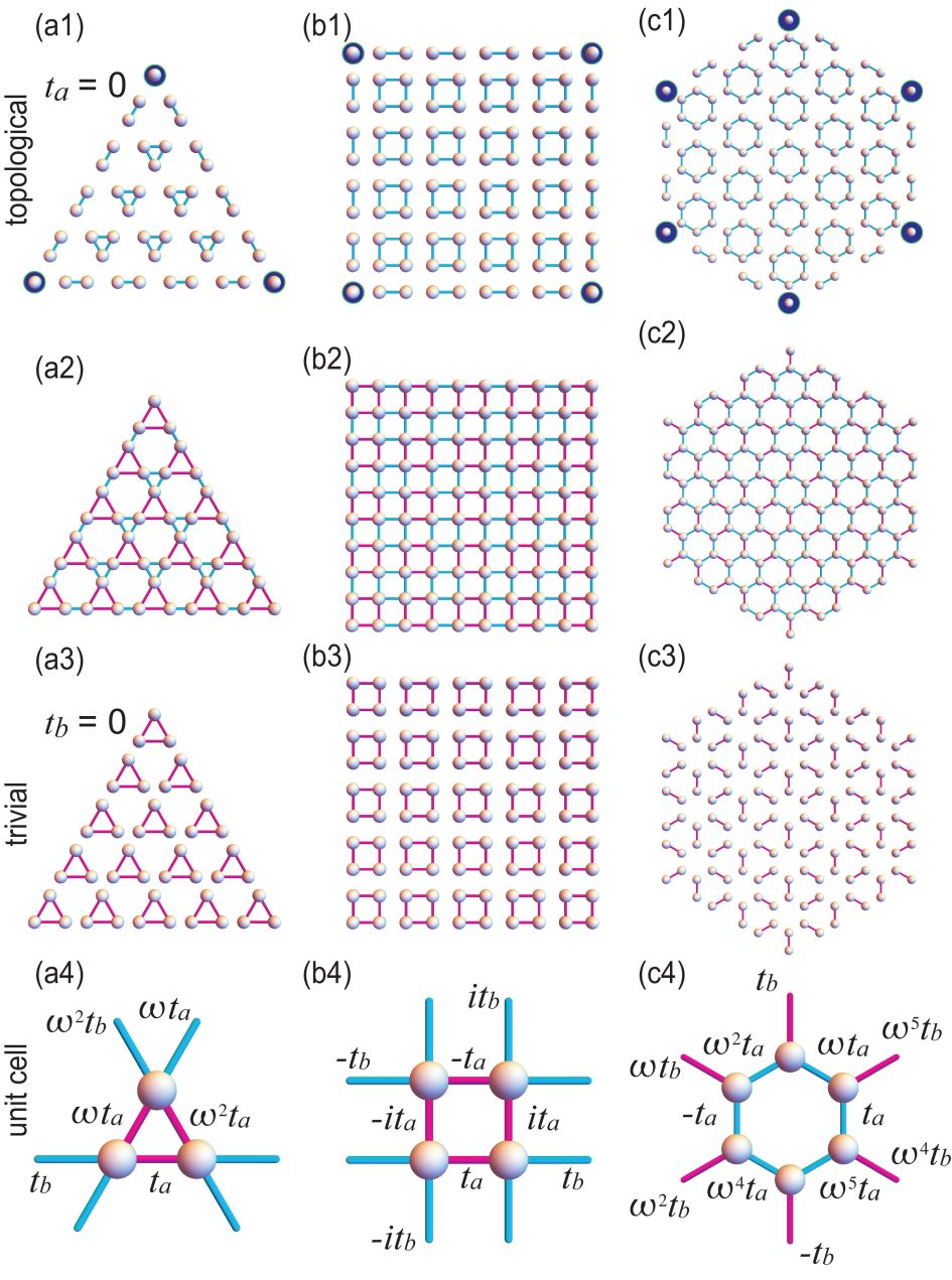
We propose a model possessing parafermions on the breathing Kagome lattice. The bulk Hamiltonian is given by
| (9) |
with
| (10) | ||||
| (11) | ||||
| (12) |
where we have introduced two hopping parameters and , corresponding to the magenta link and the cyan link along the horizontal axis in Fig.1(a4). The hopping parameters along the other two triangle sides are given by and for a magenta triangle, and and for a cyan triangle. This model is non-Hermitian due to the presence of .
A comment is in order with respect to the breathing Kagome model. It is a typical model for the conventional second-order topological insulatorKagome , where the factor is absent and it is Hermitian. The present generalization of the breathing Kagome lattice model provides us with a new type of non-Hermitian second-order topological insulators.

III.3 Clock symmetry
The Hamiltonian (9) has clock symmetryFend ,
| (13) |
where rotates the momentum by 120 degrees as
| (14) | ||||
| (15) | ||||
| (16) |
making the energy spectrum have symmetry in the complex plane as in Eq.(6). In addition, there is an anti-unitary symmetry
| (17) |
where implies complex conjugate. It leads to reflection symmetry between and . As a result, the energy spectrum has symmetry in the complex plane, which consists of the three-fold rotational symmetry and three reflection symmetries.
III.4 Phase diagram
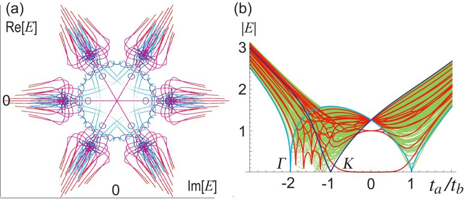
The notion of insulator and metal is generalized to the non-Hermitian Hamiltonian in two ways. On is a point-gap insulatorGong ; Kawabata , where has a gap. The other is a line-gap insulatorGong ; Kawabata , where Re or Im has a gap. In our model, we adopt the definition of the point-gap insulator due to symmetry. We are able to determine the energy spectrum analytically at the point as
| (19) |
and at the and points as
| (20) |
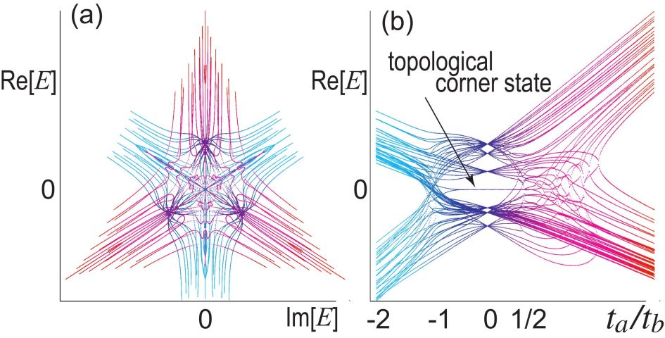
The point gap closes at the and points for , , and at the , and points for , as in Fig.2(b). This is also confirmed numerically by calculating the band spectrum as in Fig.2(b).
III.5 Topological number
The topological number is given by the Berry phase defined by
| (21) |
where is the eigen function of the Hamiltonian (9) for the bulk, whose eigen energy is real along the axis (i.e., ). We calculate it numerically, whose results are shown in Fig.2(a). We find for , and for and , while it continuously changes from to for . In fact, is quantized in the insulator phases.
III.6 Edge states
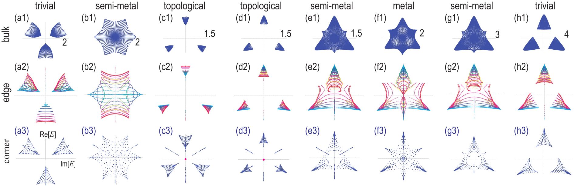
We calculate the energy spectrum in a nanoribbon numerically. Edge states are observed in Fig.4(a2)(h2), where the complex energy spectrum is shown for various momentum specified by color. Three-fold symmetry is slightly broken in nanoribbon geometry. It is due to the finite size effect of a nanoribbon.
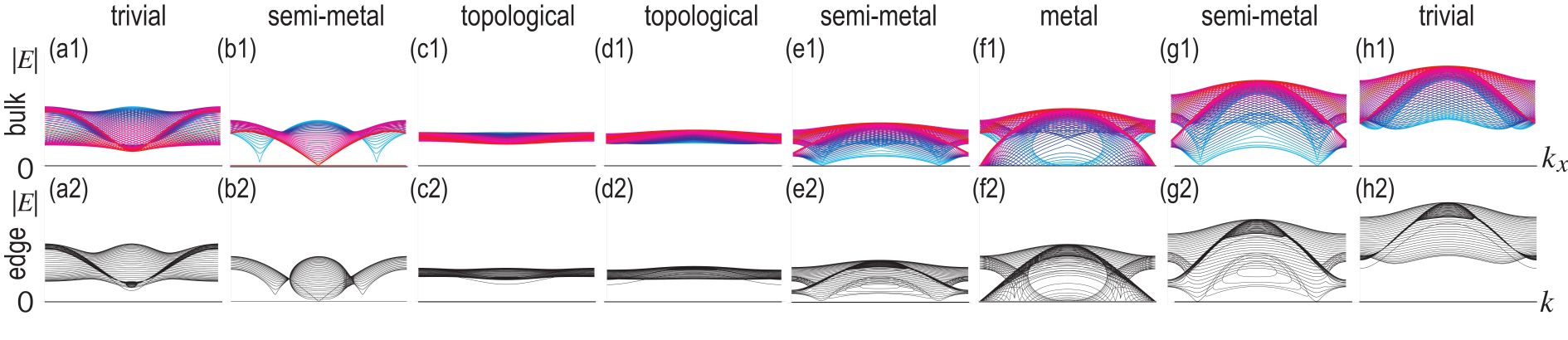
We present the band structure of a nanoribbon in Fig.5(a2)(h2), where we observe the absence of gapless edge states in the topological phase.
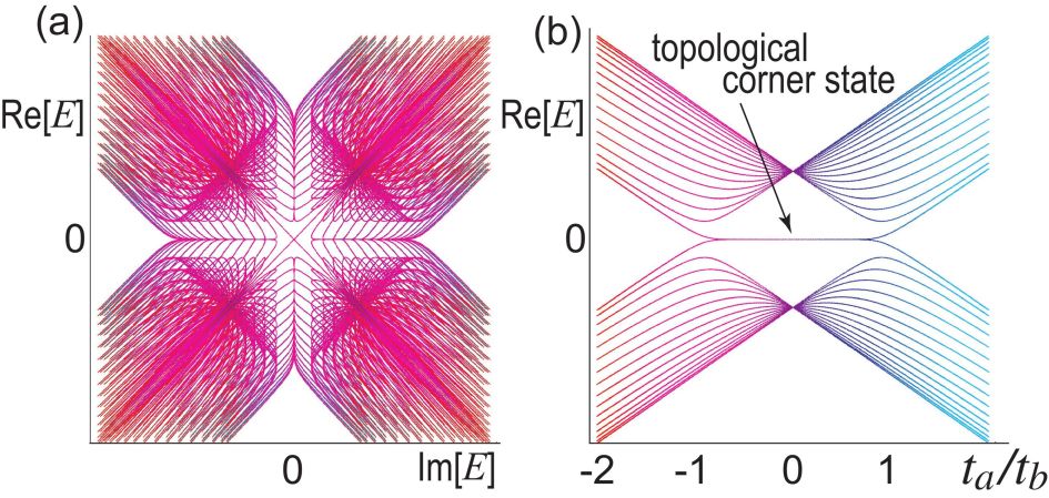
III.7 Corner states
We calculate the energy spectrum in triangle geometry numerically. symmetry is manifest as shown in Fig.3(a) and in Fig.4(a3)(h3). It is because the triangle respects clock symmetry. We find zero-energy states in the region , as indicated by a magenta line in Fig.2(d). We also show the energy spectrum as a function of in Fig.3(b), where the emergence of the zero-energy states is manifest in the topological phase.
Consequently, the present model is a second-order topological insulator in the region , being characterized by the emergence of topological corner states.
III.8 Electric-circuit implementation
Electric circuits are governed by the Kirchhoff current law. By making the Fourier transformation with respect to time, the Kirchhoff current law is expressed as
| (22) |
where is the current between node and the ground, while is the voltage at node . The matrix is called the circuit Laplacian. Once the circuit Laplacian is given, we can uniquely setup the corresponding electric circuit. By equating it with the Hamiltonian asTECNature ; ComPhys
| (23) |
it is possible to simulate various topological phases of the Hamiltonian by electric circuitsTECNature ; ComPhys ; Hel ; Lu ; YLi ; EzawaTEC ; EzawaLCR ; EzawaSkin ; Garcia ; Hofmann ; EzawaMajo ; Tjunc . The relations between the parameters in the Hamiltonian and in the electric circuit are determined by this formula.
The circuit Laplacian is constructed as follows. To simulate the positive and negative hoppings in the Hamiltonian, we replace them with the capacitance and the inductance , respectively. We note that represents an imaginary hopping in the tight-bind model. The imaginary hopping is realized by an operational amplifierHofmann .
We thus make the following replacements with respect to hoppings in the Hamiltonian to derive the circuit Laplacian: (i) for and , where represents the capacitance whose value is [pF]. (ii) for and , where represents the inductance whose value is [H].
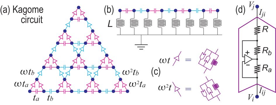
We explicitly study the breathing Kagome lattice described by (9), where the electric circuit is given by Fig.6(a). The Hamiltonian (9) is decomposed into
| (24) |
with
| (25) |
and
| (26) |
where is Hermitian (), and is anti-Hermitian (). It is necessary to construct imaginary hopping Hamiltonians
| (27) |
and
| (28) |
for the magenta lines in Fig.6(a). They are constructed by using operational amplifiers and resistors.
We review a negative impedance converter with current inversion based on an operational amplifier with resistorsHofmann . The voltage-current relation for the operational amplifier circuit is given byHofmann
| (29) |
with , where , and are the resistances in an operational amplifier: See Fig.6(d). We note that the resistors in the operational amplifier circuit are tuned to be in the literatureHofmann so that the system becomes Hermitian, where the corresponding Hamiltonian represents a spin-orbit interaction.
In this paper, we use two negative impedance converters parallelly connected with the opposite direction as in Fig.6(c). The circuit Laplacian due to these two converters is given by
| (30) |
It corresponds to the Hamiltonian
| (31) |
It is embedded in the 33 matrix as
| (32) |
where we have set
| (33) |
with , and
| (34) |
where we have set
| (35) |
with . These matrices are different from Eqs.(27) and (28) by the diagonal terms. They are cancelled by adding a resistor (for ) or an operational amplifier (for ) with the amount of
| (36) |
between a lattice site and the ground.
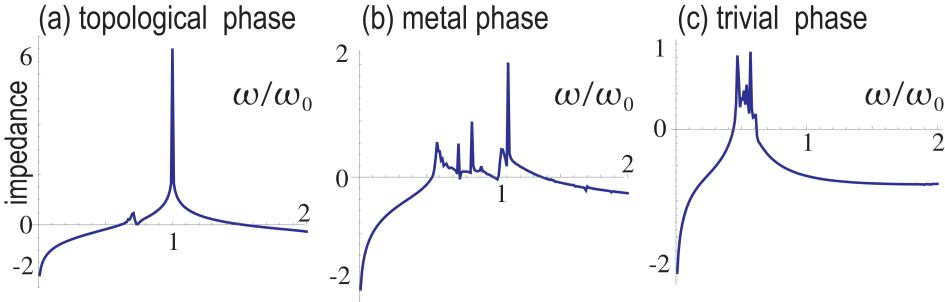
III.9 Impedance resonance
The zero-energy parafermion corner states are well observed by impedance resonance, which is definedHel by
| (37) |
where is the Green function. It diverges at the frequency where the admittance is zero (). Taking the nodes and at two corners, we show the impedance in topological, metallic and trivial phases in Figs.7(a)(c), respectively. A strong impedance peak is observed at the critical frequency only in the topological phase. It signals the emergence of zero-energy parafermion corner states.
IV Parafermion
We proceed to a model with . parafermions are represented by the shift operatorZohar ; Fend ; AliceaPara
| (38) |
and the clock operatorZohar ; Fend ; AliceaPara
| (39) |
Here, and satisfy the parafermion relations,
| (40) |
In the clock-symmetric model, the energy spectrum is composed of quartets , ,
| (41) |
The system is necessarily non-Hermitian because the eigen energies are complex except for zero-energy states.
IV.1 Zero-energy parafermion states
It follows from Eq.(41) that only the zero-energy states form a set of degenerate states respecting clock symmetry. They are parafermion states. We denote them as , , and . They are characterized by the properties
| (42) | ||||
| (43) | ||||
| (44) | ||||
| (45) |
from which the matrix representations (3) and (4) follow. Then, the parafermion relations (5) are verified. Namely, it is necessary and sufficient to examine Eqs.(7) and (8) for a triplet set of zero-energy states in order to show that they are parafermions.
IV.2 Breathing square lattice
IV.3 Edge and corner states
The topological number is defined by (21), where is the eigen function of the Hamiltonian (46) for the bulk. We find the topological insulator phase for , where and the trivial insulator phase for , where .
We calculate the energy spectrum in square geometry numerically. symmetry is manifest as shown in Fig.8(a). It is because the square lattice respects clock symmetry. We also show the energy spectrum as a function of in Fig.8(b), where the emergence of the zero-energy states is manifest in the topological phase.
Consequently, the present model is a second-order topological insulator in the region , being characterized by the emergence of topological corner states.
It is possible to obtain numerically the wave functions of the four corner states. We have confirmed that they satisfy the relations (7) and (8). Therefore, they are parafermions.
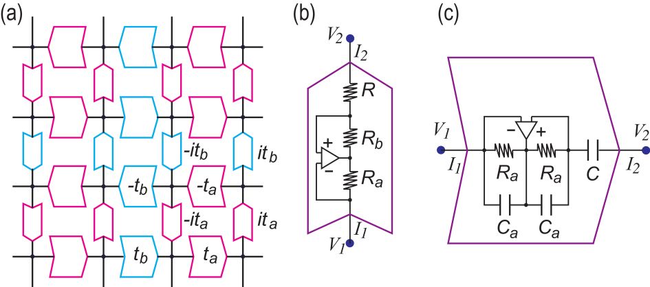
IV.4 Electric-circuit implementation
V Parafermion
Finally, we construct a parafermion model. The parafermion operators are represented by the shift operatorZohar ; Fend ; AliceaPara
| (53) |
and the clock operatorZohar ; Fend ; AliceaPara
| (54) |
Here, and satisfy the parafermion relations,
| (55) |
In the clock-symmetric model, the energy spectrum is composed of sextets , ,
| (56) |
The system is necessarily non-Hermitian because the eigen energies are complex except for zero-energy states.
A Hermitian second-order topological insulator has been proposed on the breathing honeycomb latticeMizoguchi . We generalize it to a non-Hermitian model with clock symmetry by introducing complex hoppings. The bulk Hamiltonian is defined on the breathing honeycomb lattice and given by
| (57) |
We diagonalize this Hamiltonian for a hexagon shown in Fig.1(c2). symmetry is manifest in the complex energy plane as in Fig.10(a). Furthermore, we find six zero-energy topological corner states for , as shown in Fig.10(b). We also find the trivial insulator phase for and . Additionally, there is metallic phase for .
VI Conclusion
We have constructed a parafermion model on the breathing Kagome lattice, a parafermion model on the breathing square lattice and a parafermion model on the breathing honeycomb lattice. These model exhaust all the possible realization of parafermions since there are only three-fold, four-fold and six-fold rotational symmetries that are compatible with the periodic lattices. We note that two-fold symmetry corresponds to Majorana fermions.
The author is very much grateful to Y. Tanaka and N. Nagaosa for helpful discussions on the subject. This work is supported by the Grants-in-Aid for Scientific Research from MEXT KAKENHI (Grants No. JP17K05490 and No. JP18H03676). This work is also supported by CREST, JST (JPMJCR16F1 and JPMJCR20T2).
References
- (1) G. Moore and N. Read, Nucl. Phys. B 360, 362 (1991).
- (2) S. Das Sarma, M. Freedman, and C. Nayak, Phys. Rev. Lett. 94, 166802 (2005).
- (3) A. Kitaev, Annals of Physics 321, 2 (2006).
- (4) C. Nayak, S. H. Simon, A. Stern, M. Freedman, and S. Das Sarma, Rev. Mod. Phys. 80, 1083 (2008).
- (5) A. Stern, Ann. Physics 323, 204 (2008).
- (6) A. Stern, Nature 464, 187 (2010).
- (7) S. Das Sarma, M. Freedman, C. Nayak, npj Quantum Information 1, 15001 (2015).
- (8) C. W.J. Beenakker, Annu. Rev. Condens. Matter Phys. 4, 113 (2013).
- (9) T. D. Stanescu and S. Tewari, J. Phys. Condens. Matter 25, 233201 (2013).
- (10) S.R. Elliott and M. Franz, Rev. Mod. Phys. 87, 137 (2015).
- (11) D. Aasen, M. Hell, R. V. Mishmash, A. Higginbotham, J. Danon, M. Leijnse, T. S. Jespersen, J. A. Folk, C. M. Marcus, K. Flensberg, and J. Alicea, Phys. Rev. X 6, 031016 (2016).
- (12) D. A. Ivanov Phys. Rev. Lett. 86, 268, (2001).
- (13) B. I. Halperin, Y. Oreg, A. Stern, G. Refael, J. Alicea and F. von Oppen, Phys. Rev. B 85, 144501 (2012).
- (14) J. Alicea, Y. Oreg, G. Refael, F. von Oppen and M.P.A. Fisher, Nat. Phys. 7, 412 (2011).
- (15) X.-L. Qi, S.-C. Zhang, Rev. Mod. Phys. 83, 1057 (2011).
- (16) M. Leijnse and K. Flensberg, Semicond. Sci. Technol. 27, 124003 (2012).
- (17) J. Alicea, Rep. Prog. Phys. 75, 076501 (2012).
- (18) M. Sato and Y. Ando, Rep. Prog. Phys. 80, 076501 (2017).
- (19) Y. Tanaka, M. Sato and N. Nagaosa, J. Phys. Soc. Jpn. 81, 011013 (2012).
- (20) Y. Kasahara, T. Ohnishi, Y. Mizukami, O. Tanaka, Sixiao Ma, K. Sugii, N. Kurita, H. Tanaka, J. Nasu, Y. Motome, T. Shibauchi, Y. Matsuda, Nature 559, 227 (2018).
- (21) A. Ahlbrecht, L. S. Georgiev, R. F. Werner, Phys. Rev. A 79, 032311 (2009).
- (22) P. Fendley, J. Stat. Mech. 2012, 11020 (2012).
- (23) P. Fendley, J. Phys. A 47, 075001 (2014).
- (24) J. Alicea, P. Fendley, Annual Review of Condensed Matter Physics 7, 119 (2016).
- (25) Adam S. Jermyn, Roger S. K. Mong, Jason Alicea, and Paul Fendley, Phys. Rev. B 90, 165106 (2014).
- (26) H. Ebisu, E. Sagi, Y. Tanaka, and Y. Oreg, Phys. Rev. B 95, 075111 (2017)
- (27) A. Hutter and D. Loss, Phys. Rev. B 93, 125105 (2016).
- (28) R. J. Baxter, Phys. Lett. A 140, 155 (1989); J. Statist. Phys. 57, 1 (1989).
- (29) N. Read and E. Rezayi, Phys. Rev. B 59, 8084 (1999).
- (30) D. J. Clarke, J. Alicea, K. Shtengel, Nat. Com. 4, 1348 (2013).
- (31) K. Laubscher, D. Loss, J. Klinovaja, Phys. Rev. Research 1, 032017 (2019).
- (32) K. Laubscher, D. Loss, J. Klinovaja, Phys. Rev. Research 2, 013330 (2020).
- (33) F. Zhang, C.L. Kane and E.J. Mele, Phys. Rev. Lett. 110 , 046404 (2013).
- (34) W. A. Benalcazar, B. A. Bernevig, and T. L. Hughes, Science 357, 61 (2017).
- (35) F. Schindler, A. Cook, M. G. Vergniory, and T. Neupert, in APS March Meeting (2017).
- (36) Y. Peng, Y. Bao, and F. von Oppen, Phys. Rev. B 95, 235143 (2017).
- (37) J. Langbehn, Y. Peng, L. Trifunovic, F. von Oppen, and P. W. Brouwer, Phys. Rev. Lett. 119, 246401 (2017).
- (38) Z. Song, Z. Fang, and C. Fang, Phys. Rev. Lett. 119, 246402 (2017).
- (39) W. A. Benalcazar, B. A. Bernevig, and T. L. Hughes, Phys. Rev. B 96, 245115 (2017).
- (40) F. Schindler, A. M. Cook, M. G. Vergniory, Z. Wang, S. S. P. Parkin, B. A. Bernevig, and T. Neupert, Science Advances 1, eaat0346 (2018).
- (41) C. Fang, L. Fu, Science Advances 5, eaat2374 (2019).
- (42) M. Ezawa, Phys. Rev. Lett. 120, 026801 (2018).
- (43) M. Ezawa, Phys. Rev. B 98, 045125 (2018).
- (44) M. Geier, L. Trifunovic, M. Hoskam, and P. W. Brouwer, Phys. Rev. B 97, 205135 (2018).
- (45) E. Khalaf, Phys. Rev. B 97, 205136 (2018).
- (46) M. Ezawa, Phys. Rev. B 100, 045407 (2019).
- (47) T. Liu, Y.-R. Zhang, Q. Ai, Z. Gong, K. Kawabata, M. Ueda, F. Nori, Phys. Rev. Lett. 122, 076801 (2019).
- (48) M. Ezawa, Phys. Rev. B 99, 201411(R) (2019).
- (49) M. Ezawa, Phys. Rev. B 99, 121411(R) (2019).
- (50) E. Edvardsson, F. K. Kunst, E. J. Bergholtz, Phys. Rev. B 99, 081302 (2019).
- (51) G. Ortiz, E. Cobanera, Z. Nussinov, Nuc. Phys. B 854, 780 (2012).
- (52) X. Ni, M. Weiner, A. Alu and A. B. Khanikaev, Nature Materials 18, 113 (2019).
- (53) Z. Gong, Y. Ashida, K. Kawabata, K. Takasan, S. Higashikawa and M. Ueda, Phys. Rev. X 8, 031079 (2018).
- (54) K. Kawabata, K. Shiozaki, M. Ueda, and M. Sato, Phys. Rev. X 9, 041015 (2019).
- (55) S. Imhof, C. Berger, F. Bayer, J. Brehm, L. Molenkamp, T. Kiessling, F. Schindler, C. H. Lee, M. Greiter, T. Neupert, R. Thomale, Nat. Phys. 14, 925 (2018).
- (56) C. H. Lee , S. Imhof, C. Berger, F. Bayer, J. Brehm, L. W. Molenkamp, T. Kiessling and R. Thomale, Communications Physics, 1, 39 (2018).
- (57) T. Helbig, T. Hofmann, C. H. Lee, R. Thomale, S. Imhof, L. W. Molenkamp and T. Kiessling, Phys. Rev. B 99, 161114 (2019).
- (58) Y. Lu, N. Jia, L. Su, C. Owens, G. Juzeliunas, D. I. Schuster and J. Simon, Phys. Rev. B 99, 020302 (2019).
- (59) Y. Li, Y. Sun, W. Zhu, Z. Guo, J. Jiang, T. Kariyado, H. Chen and X. Hu, Nat. Com. 9, 4598 (2018).
- (60) M. Ezawa, Phys. Rev. B 98, 201402(R) (2018).
- (61) M. Serra-Garcia, R. Susstrunk and S. D. Huber, Phys. Rev. B 99, 020304 (2019).
- (62) T. Hofmann, T. Helbig, C. H. Lee, M. Greiter, R. Thomale, Phys. Rev. Lett. 122, 247702 (2019).
- (63) M. Ezawa, Phys. Rev. B 102, 075424 (2020).
- (64) T. Helbig, T. Hofmann, S. Imhof, M. Abdelghany, T. Kiessling, L. W. Molenkamp, C. H. Lee, A. Szameit, M. Greiter, R. Thomale, Nature Physics 16, 747 (2020)
- (65) T. Mizoguchi, H. Araki and Y. Hatsugai, J. Phys. Soc. Jpn. 88, 104703 (2019)