Topological properties on isochronous centers of polynomial Hamiltonian differential systems
Abstract.
In this paper, we study the topological properties of complex polynomial Hamiltonian differential systems of degree having an isochronous center. Firstly, we prove that if the critical level curve possessing an isochronous center contains only a single singular point, and the period -form does not have poles with zero residue at infinity on level curves sufficiently close to the critical curve, then the vanishing cycle associated to this center is trivial in the 1-dimensional homology group of the projective closure of a generic level curve. Our result provides a positive answer to a question asked by L. Gavrilov under relatively simple conditions and can be applied to achieve an equivalent description of the Jacobian conjecture on . Secondly, we obtain a very simple but useful necessary condition for isochronicity of Hamiltonian systems, which is that the -degree part of the Hamiltonian function must have a factor with multiplicity no less than . Thirdly, we show a relation between Gavrilov’s question and the conjecture proposed by X. Jarque and J. Villadelprat on the non-isochronicity of real Hamiltonian systems of even degree .
Key words and phrases:
Hamiltonian differential systems; isochronous center; vanishing cycle; Jacobian conjecture2010 Mathematics Subject Classification:
Primary: 34M35, 34C05; Secondary: 34C08;1. Introduction and main results
Consider the following complex polynomial Hamiltonian differential systems of degree
| (1.5) |
where the Hamiltonian function is a polynomial of degree in . Assuming the origin is a center of Morse type, without loss of generality, can be written as . For a generic level curve defined by the algebraic equation where is sufficiently close to , one can associate a vanishing cycle to the critical value , which is a 1-dimensional cycle vanishing at in the 1-dimensional homology group and can be characterized by the following purely topological property: modulo orientation and the free homotopy deformation on , as , the cycle can be represented by a continuous family of loops on of length that tends to zero. This description explains the terminology(see, e.g., [8]). Respectively is called a period function of system (1.5). If is a nonzero constant independent of for , then the origin is called an isochronous center. This definition coincides with the classical isochronous center when and .
One of the most important problems on isochronous centers is to describe the role of the vanishing cycle in the 1-dimensional homology group of the compact Riemann surface of . It is still an open problem until now. In [7], L. Gavrilov has asked the following question for systems (1.5) with only isolated singularities:
Question 1.1 (Gavrilov’s question).
Is it true that if a Morse singular point is isochronous, then the associated vanishing cycle represents a zero homology cycle on the Riemann surface of the level curve ?
In general cases, the above question has a negative answer. Example 3.23 in reference [4] provides a system with
which has an isochronous center at the origin, but the corresponding vanishing cycle is not homologous to zero on the Riemann surface of . In this counterexample, it is not difficult to see that the critical level curve contains at least three different singularities on .
What conditions can give a positive answer to Gavrilov’s question? This is also an important and meaningful question, especially it is closely related with the famous Jacobian conjecture on , which asserts that the following polynomial map with a constant Jacobian determinant
| (1.8) |
is a global homeomorphism, where and are polynomials in . At present it has been proved only when the degrees of and are not too large. Obviously the map induces a Hamiltonian system
| (1.15) |
having an isochronous center of Morse type at the origin with the Hamiltonian function .
Also in [7], Proposition 6.1 says that if the vanishing cycle associated to the origin for system (1.15) represents a zero homology cycle on the Riemann surface of a generic level curve, then the map is injective, which suffices to guarantee the Jacobian conjecture is true. In addition, he has also proved that(Theorem 4.1 of [7]) Question 1.1 has a positive answer under the conditions that the critical level curve contains only a single singular point which is isochronous and is a ‘good’ polynomial having only isolated and simple singularities, where the definition of a good polynomial depends on the Milnor numbers of the complex projective closure of at infinity.
This paper is devoted to look for other conditions to give a positive answer to Question 1.1. Denote by
the period -form of system (1.5). We have the following main theorem.
Theorem 1.2.
For system (1.5), if the critical level curve contains a single singularity which is an isochronous center of Morse type, and the period -form does not have poles with zero residue at infinity for any sufficiently close to , then the associated vanishing cycle is trivial in .
Applying the above theorem to system (1.15), one can achieve an equivalent description of the Jacobian conjecture.
Corollary 1.3.
The polynomial map with constant Jacobian determinant is a global homeomorphism, if and only if two algebraic curves and intersect only at a single point on .
To prove Theorem 1.2, we will carefully study some real systems induced by complex system (1.5) and the corresponding transformation linearizing an isochronous center. Such systems possess many good properties, such as commutativity, transversality, and so on. Besides, their topological structures near the points at infinity on can also provide for us a lot of information for the isochronicity of system (1.5). Letting be the highest degree part of , we have the following necessary condition for isochronicity:
Theorem 1.4.
For system (1.5), if the origin is an isochronous center, then must have a factor with multiplicity no less than .
In this paper, we will also show an interesting relation between Gavrilov’s question and the following conjecture, which was claimed by X. Jarque and J. Villadelprat in [9], on real systems (1.5), i.e., and .
Conjecture 1.5 (Jarque-Villadelprat conjecture).
If is even, then the real system (1.5) has no isochronous centers.
At present, this conjecture is still open and a recent development can be found in [5]. The following theorem indicates that if the Jarque-Villadelprat conjecture is not true, then the Gavrilov’s question must have a negative answer for such real systems.
Theorem 1.6.
For any isochronous center of a real system (1.5) with even , the corresponding vanishing cycle can not be homologous to zero on the projective closure of the complexification of a generic real level curve.
The paper is organized as follows. We shall first introduce some properties on the commuting real differential systems(or real vector fields) induced by system (1.5) and provide a powerful technique to extend the transformation linearizing an isochronous center. Then we give the detailed proof of the main results and some applications.
2. Commuting real systems
Note that if the origin is an isochronous center of Morse type for system (1.5), then there exists an analytic area-preserving transformation(see, e.g, [1, 11, 12])
changing system (1.5) to a linear system
| (2.5) |
here we say is area-preserving is equivalent to say its Jacobian determinant , where
Generally speaking, is only well defined in a small neighborhood of the origin .
By taking advantage of constant Jacobian determinant, one can construct another complex system in as follows
| (2.10) |
which can be also linearized to a linear system
| (2.15) |
by the same transformation , for the reasons that
and
Consequently, systems (1.5) and (2.15) induce the following four real differential systems(see, e.g. [3]) by taking but :
and
where . They can be transformed to the following four real linear systems simultaneously by the same respectively:
and
Letting and and regarding , the coefficient matrices of , , and are respectively
where
Obviously we have
Due to that is a diffeomorphism, one can get the following important properties for vector fields , , , and :
-
(1)
they are commutative pairwise everywhere in , i.e., as real vector fields, the Lie bracket of any two of them vanishes. So for any two points in except , it takes the same time along any two continuous paths connecting and consisting of finitely many trajectories of those vector fields.
-
(2)
their trajectories are transversal pairwise everywhere on ; while on , (resp. ) coincides with (resp. ) on one of two branches near and with (resp. ) on the other one;
-
(3)
the domain in which and can be well defined is the same to the domain of , but and are well defined on the whole complex plane ;
-
(4)
near the origin, all of the orbits of system are closed; on the contrary, system does not have any closed orbits in ;
-
(5)
the trajectories of systems and are both tangent to everywhere, so their restrictions, denoted by and , are two real systems defined well on .
Denote by (resp. , and ) the flow map induced by (resp. , , , , and ), i.e., for any given point , takes the value at time of the solution of equations with initial value at . The commutativity between those systems means that each one of the flow maps above preserves the orbits of any other system in the domain of . We shall take advantage of this observation to extend the domain of to a bigger one than . Without loss of generality, we assume is a sufficiently small and homeomorphic to a open ball centered at with radius . Denote by the following map
Continuation technique for :
For a closed orbit of in such that , and two sufficiently small number , the space
is a real 3-dimension sub-manifold of and transversal to at every point. Then is also a real 3-dimension sub-manifold of and transversal to at every point.
Along the trajectories of passing through in , the transformation can be expressed by the flow map as follows: for any point and any sufficiently small , we have
| (2.27) |
Clearly the vector fields and are well defined globally, the above equation can be extended to a larger interval for time such that , if satisfies the following two conditions:
-
C1.
the trajectories of could not return into the domain where has already been defined well;
-
C2.
there is no point at infinity such that tends to as tends a finite moment for some a point .
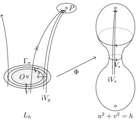
If the trajectories of from a open subset of go to a point at infinity when tends , then the interval for those points can be or . While if C1 holds but C2 not, then can only be or at such a point (see Figure 1).
Noticing that the vector fields and are also well defined globally, we can also perform the above operation along the trajectories of if it satisfies the conditions C1 and C2.
In a word, one can extend the transformation to an open domain as big as possible according to the above operation along the trajectories of and . Although may be much bigger than , we have is still homeomorphic to for any sufficiently close to .
3. Points at infinity
To prove the main results, we still need to know some information about the points at infinity on . It is better to deal with it in the projective space . Assume the projective closure are defined by the following homogeneous equations
where represents the homogeneous part of degree of . For a generic value , the set of singularities on , denoted by , consists of only some points at infinity on . The Riemann surface of coincides with the resolution of by a birational map. Generally speaking, The algebraic curve may have more than one connected branches near a point . The number of such branches is equal to the number of essentially different Puiseux expressions associated to (see, e.g., [10]).
Rewriting the homogeneous part of degree as follows:
| (3.1) |
where such that if the projective coordinate of a point can be represented by . Up to a projective change of coordinates, we can always assume its projective coordinate is . Then it is convenient to adopt a pair of new affine coordinates , where
and the Puiseux expressions near are totally determined by the Puiseux expressions of equation
| (3.2) |
near the origin. According to the classical theory of Puiseux(see, e.g., ([6])), each branch of an algebraic curve near a singularity can be parameterized by a Puiseux series of the following form.
Lemma 3.1 (Puiseux).
If and , then there exist numbers , a parameter , and a a holomorphic function such that for all in a neighbourhood of .
In general the coefficients may depend on on different level curve , so sometimes we replace with to emphasize it. Taking the Puiseux parameterization into system (1.5), we obtain a complex 1-dimension ordinary differential equation
| (3.3) |
on a branch of near , where Then the real systems and are changed to the following forms respectively under this parameterization:
| (3.4) |
and
| (3.5) |
Their topological structures can be classified into the following four classes according to the value of near :
- •
-
•
. If is a pure imaginary number, the point is of center-focus type; while for , it is a node, and for other numbers, it is a focus.
- •
- •
Remark 3.2.
It should be pointed out that there may exist an orbit of system (3.4) such that it can reach the origin at a finite moment from a fixed point . It is not difficult to see this phenomenon occurs only in the cases and , and in the latter one such an orbit is just the separatrix of the saddle.
The Puiseux parameterizations can be determined completely by the so-called Newton polygon of the singularity. Given an irreducible polynomial with , denote by the carrier of , i.e. Assuming that , let
be the straight line segment from to . Consider the convex subset on consisting of those such that and for some where .
Definition 3.3 (Newton Polygon).
The boundary of set excluding the axes is called the Newton polygon of at the origin, which consists of only finitely many straight line segments.
4. Important lemmas
In this section, we first prove the following important lemmas. It is not difficult to see the vanishing cycle can be represented by a given closed orbit of system near the origin(we still denote this orbit by ).
Lemma 4.1.
If the origin is an isochronous center of system (1.5), then every orbit of passing through a point on is not closed for any sufficiently close to .
Proof.
Suppose otherwise, i.e., suppose there exists a point such that the orbit of passing through is closed. Then by the commutativity between and , there exists a sufficiently small neighborhood of such that for any , the orbit of passing through is also closed.
Consider the inverse transformation that also has a constant Jacobian determinant in the domain on the -plane. Since satisfies the conditions C1 and C2, by using the same continuation technique introduced in Section 2, we can extend from to a bigger domain along the trajectories of by the following equation
such that covers all closed orbits of passing through (see Figure 2).
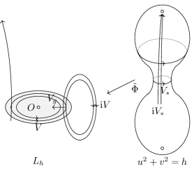
In the domain , the vector field is well defined and commuting with . This implies that the periods of those closed orbits of are the same for any . The above operation is valid for any sufficiently close to . So we get a series of closed orbits of with the same period as along a trajectory of , whose lengths tend to since when . This means that such a closed orbit also represents the vanishing cycle of the isochronous center, which leads a contradiction, because the origin is of Morse type having only one vanishing cycle and the intersection number of two closed orbits of and respectively is equal to so that they can not represent the same one cycle in . Thus the lemma holds. ∎
By this lemma, we have the following immdiately.
Lemma 4.2.
If the origin is an isochronous center of system (1.5), then there exists a subset consisting of at most finitely many points such that:
Proof.
By Lemma 4.1, if the orbit of passing through a point can not tend any point at infinity, then there remains two possible cases:
-
•
tends a closed orbit of . If such a exists, then it is isolated or semi-isolated. However, by the commutativity between and , there exist annuli such that is not the boundary.
-
•
is ergodic on a subset of . If so, we can also extend the transformation to a domain such that covers as shown in the above lemma along (in fact, we only need to do this on ). One can choose a trajectory of for such that is dense in . Noticing that on the curve defined by is integrability, there is a non trivial analytic first integral defined on such that is a constant. Defining a function for , it is a non trivial analytic first integral for such that is not a constant. However, is a constant on a dense subset of , which implies should be also a constant. This is a contradiction.
Finally, every orbit of passing through a point can only tend to a point at infinity on one of the branches of near . According to the arguments in Remark 3.2, if the number for , then will reache at at some a finite moment . In addition, due to that the numbers of points at infinity and separatrices of the saddles are both finite, the number of such points are also finite. The lemma is proved. ∎
Below we shall show that, under the assumption of Theorem 1.2, in the second case of the above lemma, the number must be equal to .
Lemma 4.3.
Proof.
Suppose system (1.5) has a Hamiltonian and has a projective coordinate , by a linear change of coordinates , where , its coordinate can be changed to . If the linearization transformation maps to , by taking a linear change of coordinates
then one of the points at infinity also has a coordinate on -plane, i.e., the Hamiltonian function has the form .
Under the conditions of the lemma, the equation (2.27) holds for and a sufficiently small neighborhood of in , i.e., the domain where is well defined can be sufficiently close to along the orbits of .
We take the coordinates of Puiseux parameters near in , and the coordinates near in . Then induces a map from an open set in the plane to plane , so that the following diagram is commutative.
| (4.1) |
where
| (4.4) |
are Puiseux parameterizations respectively, and
| (4.7) |
Denoting by , we have
| (4.8) |
that is,
Recall the system (3.3) is the following
and the period -form can not have a pole at with zero residue, i.e. in the Laurent series of , the coefficient of is a nonzero number . Thus, can be expressed in as follows:
where , , , and equation (4.8) becomes
which implies that , . Furthermore, can be analytically extended to a sufficiently small disc encircling . Clearly the orbits of are all closed, so are the orbits of vector fields on and planes induced by and respectively. Besides, due to that the Puiseux parameterization is a finitely many cover mapping near , the orbits of are also closed. ∎
Remark 4.4.
In the proof of the above lemma, the conclusion, that the function can be analytically extended to the origin of plane, does not mean the transformation can be also analytically extended to , one of the reasons is the inverse function of Puiseux parameterization is usually multi-valued near .
This lemma tells us the period -form of system (1.5) has at least one pole at a point at infinity on a branch of near . The following lemma will show that the multiplicity of such a point can not be too low, i.e., we have
Lemma 4.5.
If has a pole at a point at infinity on a branch of near , then the multiplicity of satisfies .
Proof.
We still assume the projective coordinate of is . Let be the vertex set of the Newton polygon of near the origin, where , . Denoting by the minimum of , there exists a straight line on -plane
passing all the points contained in . We define the Newton principal polynomial by the following
where is the coefficient of term of .
Taking the Puiseux parameterization into , we get that has a pole at if and only if
| (4.9) |
where represents the lowest degree of a Laurent series.
By comparing the coefficients of terms in both sides of equation
| (4.10) |
one can easily get is a root of , so we can assume where . Letting be the first coefficient depending on in and taking the derivative on in both sides of equation (4.10), we have
| (4.11) |
Comparing the coefficients of terms on both sides of the above equation, we can get the following estimations:
-
•
, i.e., , by inequality (4.9);
-
•
, this is because the lowest degree of the left side of the above equation is not more than .
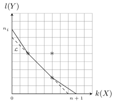
In addition, from the convexity of the Newton polygon(see Figure 3 below), inequalities and are both obvious. Finally, combining these inequalities we have
∎
In general, there may vanishing cycles associated to a singularity in on when , which may be non-trivial cycles in . However, for Hamiltonian systems with an isochronous center, we have the following lemma.
Lemma 4.6.
For system (1.5), if the origin is an isochronous center, then there does not exist a vanishing cycle associated to a singular point at infinity such that .
Proof.
Suppose otherwise, i.e., suppose that such a vanishing cycle exists and is associated to a point at infinity with the projective coordinate .
Denote by the number(counting multiplicity) of branches determined by the parts of the segments with slope in the Newton polygons of at . On one hand, when as , it yields at least one more branch on than , where the period -form has a pole at with a nonzero residue. So this branch is determined by a segment with slope in the Newton polygons of , by Lemma 4.5 and its proof. This implies .
On the other hand, the isochronous center is of Morse type, and the part of with degree has the form such that and can not be zero simultaneously. So we have
| (4.14) |
Then there are the following three possible cases, and each of them yields a contradiction.
-
•
If the Newton polygon for does not contain two points and simultaneously, then and have the same parts of the segments with slope , which give the same number .
-
•
If the Newton polygon for contains two points and simultaneously, and the line segment with slope contains only two points and , then then and have the same shapes of the part of the segments with slope , and the branch determined by on has a Puiseux parameterization
which tends to the branch on . Consequently, we still have .
-
•
If the Newton polygon for contains two points and simultaneously, but the line segment with slope contains not only these two points, then we will show that in this case the system (1.5) can not be linearizable at the point .
Let be the maximum value such that and . Then in this case has the form
(4.17) where . In fact, is nothing other than the first nonzero linearization constant. This is because, from the results in [2], the -jet of system (1.5) has admissible nonlinearities and can be linearized by a transformation of the form
(4.20) However, this transformation can not change the resonant terms in and in .
∎
5. The proof of main theorems
Now we can prove our main theorems.
Proof of Theorem 1.2.
By Lemma 4.2, without loss of generality, we assume has been divided into parts , such that for any point , goes to the same point at infinity on the same branch when . Here may not be a continuous arc of but a union of finitely many continuous arcs. By Lemma 4.3, we can choose a closed orbit of encircling and sufficiently close to on this branch.
We shall prove that, for each , there exists a moment such that . Then is homologous to the summation of those cycles , and the theorem holds since that each represents a zero homology cycle in .
Suppose otherwise, i.e. suppose that there exists a number and a branch of near a point such that the loop contains at least two continuous arcs and satisfying that but .
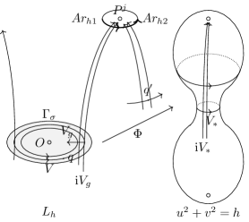
By the continuation technique, we can extend the transformation to a domain containing and for any sufficiently small , where and is a real number such that . To avoid that meets a point at infinity, can be shortened properly. Consequently, for any point , letting , there exists a point such that but (see Figure 4).
Note that must be a part of a closed orbit of vector field . If not so, then for almost every sufficiently close to , the orbit of containing tends to a point at infinity, so the orbits of near either also tend to or are closed near , which implies the number for this branch of . However, is a part of a closed orbit of , then by Lemma 4.3 and its proof, the orbit of must also be closed near , this is a contradiction.
Below we shall show that must be a vanishing cycle associated to the origin or a singularity at infinity.
Under the assumption of the theorem, has the same structures at to , by Lemma 4.6 and its proof. So the above can also extended to : given two closed orbits and of sufficiently close to and on the branch of that is the limit of branch containing on when , then for any . Thus can contain a trajectory but and for some a .
Noticing that has only a single finite singular point, can be well defined for and its limit is either the origin or a point at infinity, by Lemma 4.2 and its proof. Besides, vector field coincides with on , so will tend to along the trajectory of . This means is a vanishing cycle of a singularity at infinity or the origin.
However, by Lemma 4.6 and the assumption on the period -form, the former case is impossible. As for the latter case, recalling that but and is a homeomorphism near the origin, it is also impossible.
∎
Proof of Corollary 1.3.
If the linearization change is well defined on the whole plane , for instance, polynomial map appearing in the Jacobian conjecture, then it maps a small disc punctured by a pole of the period -form to a small disc(topologically) punctured by a pole of -form on for any . This means that dose not have poles with zero residue at infinity.
6. Non-isochronicity of real Hamiltonian systems of even degree
In the last section we focus on the relation between the Gavrilov’s question and Jarque-Villadelprat conjecture. It is worthy mentioned that the latter is not true in the complex setting, some counterexamples can be found in Gavrilov’s paper [7]. Firstly we shall prove Theorem 1.6.
Proof of Theorem 1.6.
If is a real polynomial of odd degree , then the real algebraic curve has at least two connected components on , one of them is just the closed orbit near the center which can represent the corresponding vanishing cycle, and another one, denoted by , tends to a point at infinity. The real systems can be embedded in . Then the real plane is a subset defined by , and the closed orbit on can be represented by .
If
is the transformation linearizing real isochronous center, then the following map
can linearized the complex isochronous center of system (1.5). Denoting by
the conjugate operation on , we have , since
If is a trivial cycle on the closure of the generic complex curve defined by , then is divided into two path-connected open components and such that and their common boundary is . Without loss of generality, we assume and can construct a smooth curve connecting two points and , such that intersects transversally at only one point .
In the domain where is well defined, we have , because is a homeomorphism so that and . Therefore the complex conjugate of belongs to in . Finally forms a closed curve intersecting at only one point with intersection number on (see Figure 5). This means that can not be trivial on , which leads a contradiction.
∎
By Theorem 1.6, we observe an interesting relation between Gavrilov’s question and Jarque-Villadelprat conjecture, that is, if the latter conjecture is not true, then such real systems possessing isochronous centers provide a negative answer to Gavrilov’s question.
In the end, as applications of Theorem 1.2, we present a conclusion which verifies the Jarque-Villadelprat conjecture for a large class of real systems. Note that in the real setting, an isochronous center must be a non-degenerated singularity, i.e., it must be of Morse type, so we have
Corollary 6.1.
For a real polynomial Hamiltonian system (1.5) of even degree, if each (complex) critical level curve having a center contains only a single singularity, and the period -form has no pole at infinity with zero residue on any level curve, then it does not admit any isochronous center at all.
Acknowledgements
This work is supported by NSFC 11701217 and NSF 2017A030310181 of Guangdong Province(China).
References
- [1] B. Arcet, J. Gine and V.G. Romanovski, Linearizability of planar polynomial Hamiltonian systems, Nonlinear Analysis: Real World Applications 63 (2022), 103422, 19.
- [2] J. Basto-Goncalves, Linearization of resonant vector fields, Trans. Amer. Math. Soc. 362 (12) (2010), 6457-6476.
- [3] C. Camacho, A. Lins Neto, and P. Sad, Topological invariants and equidesingularization for holomorphic systems, J. Differential Geom. 20 (1984), no. 1, 143-174.
- [4] A. Cima, F. Mañosas, J. Villadelprat, Isochronicity for several classes of Hamiltonian systems, J. Differential Equations 157, 373-413 (1999).
- [5] J. Cresson, J. Palafox, Isochronous centers of polynomial Hamiltonian systems and a conjecture of Jarque and Villadelprat, J. Differential Equations 266, 5713-5747 (2019).
- [6] G. Fischer, Plane algebraic curves, Translated from the 1994 German original by Leslie Kay. Student Mathematical Library 15. American Mathematical Society, Providence, RI, 2001.
- [7] L. Gavrilov, Isochronicity of plane polynomial Hamiltonian systems, Nonlinearity 10 (1997), 433-448.
- [8] Y. Ilyashenko, S. Yakovenko, Lectures on analytic differential equations, Graduate Studies in Mathematics 86, American Mathematical Society, Providence, RI, 2008.
- [9] X. Jarque and J. Villadelprat, Nonexistence of isochronous centers in planar polynomial Hamiltonian systems of degree four. J. Differential Equations 180, 334-373 (2002).
- [10] F. Kirwan, Complex Algebraic Curves, London Mathematical Society, Student Text 23, Cambridge University Press, Cambridge, 1992.
- [11] Llibre, J., Romanovski, V.G.: Isochronicity and linearizability of planar polynomial Hamiltonian systems. J. Differential Equations 259, 1649-1662 (2015).
- [12] F. Mañosas and J. Villadelprat, Area-preserving normalizations for centers of planar Hamiltonian J. Differential Equations 179, 625-646 (2002).