Topological Signal Processing over
Simplicial Complexes
Abstract
The goal of this paper is to establish the fundamental tools to analyze signals defined over a topological space, i.e. a set of points along with a set of neighborhood relations. This setup does not require the definition of a metric and then it is especially useful to deal with signals defined over non-metric spaces. We focus on signals defined over simplicial complexes. Graph Signal Processing (GSP) represents a special case of Topological Signal Processing (TSP), referring to the situation where the signals are associated only with the vertices of a graph. Even though the theory can be applied to signals of any order, we focus on signals defined over the edges of a graph and show how building a simplicial complex of order two, i.e. including triangles, yields benefits in the analysis of edge signals. After reviewing the basic principles of algebraic topology, we derive a sampling theory for signals of any order and emphasize the interplay between signals of different order. Then we propose a method to infer the topology of a simplicial complex from data. We conclude with applications to real edge signals and to the analysis of discrete vector fields to illustrate the benefits of the proposed methodologies.
Index Terms:
Algebraic topology, graph signal processing, topology inference.I Introduction
Historically, signal processing has been developed for signals defined over a metric space, typically time or space. More recently, there has been a surge of interest to deal with signals that are not necessarily defined over a metric space. Examples of particular interest are biological networks, social networks, etc. The field of graph signal processing (GSP) has recently emerged as a framework to analyze signals defined over the vertices of a graph [2], [3]. A graph is a simple example of topological space, composed of a set of elements (vertices) and a set of edges representing pairwise relations. However, notwithstanding their enormous success, graph-based representations are not always able to capture all the information present in interconnected systems in which the complex interactions among the system constitutive elements cannot be reduced to pairwise interactions, but require a multiway description, as suggested in [4, 5, 6, 7, 8, 9].
To establish a general framework to deal with complex interacting systems, it is useful to start from a topological space, i.e. a set of elements , along with an ensemble of multiway relations, represented by a set containing subsets of various cardinality, of the elements of . The structure is known as a hypergraph. In particular, a class of hypergraphs that is particularly appealing for its rich algebraic structure is given by simplicial complexes, whose defining feature is the inclusion property stating that if a set belongs to , then all subsets of also belong to [10]. Restricting the attention to simplicial complexes is a limitation with respect to a hypergraph model. Nevertheless, simplicial complex models include many cases of interest and, most important, their rich algebraic structure makes possible to derive tools that are very useful for analyzing signals over the complex. Learning simplicial complexes representing the complex interactions among sets of elements has been already proposed in brain network analysis [6], neuronal morphologies [11], co-authorship networks [12], collaboration networks [13], [14], tumor progression analysis [15]. More generally, the use of algebraic topology tools for the extraction of information from data is not new: The framework known as Topological Data Analysis (TDA), see e.g. [16], has exactly this goal. Interesting applications of algebraic topology tools have been proposed to control systems [17], statistical ranking from incomplete data [18], [19], distributed coverage control of sensor networks [20, 21, 22], wheeze detection [23]. One of the fundamental tools of TDA is the analysis of persistent homologies extracted from data [24], [25]. Topological methods to analyze signals and images are also the subjects of the two books [26] and [27].
The goal of our paper is to establish a fundamental framework to analyze signals defined over a simplicial complex. Our approach is complementary to TDA: Rather than focusing, like TDA, on the properties of the simplicial complex extracted from data, we focus on the properties of signals defined over a simplicial complex. Our approach includes GSP as a particular case: While GSP focuses on the analysis of signals defined over the vertices of a graph, topological signal processing (TSP) considers signals defined over simplices of various order, i.e. signals defined over nodes, edges, triangles, etc. Relevant examples of edge signals are flow signals, like blood flow between different areas of the brain [28], data traffic over communication links [29], regulatory signals in gene regulatory networks [30], where it was shown that a dysregulation of these regulatory signals is one of the causes of cancer [30]. Examples of signals defined over triplets are co-authorship networks, where a (filled) triangle indicates the presence of papers co-authored by the authors associated to its three vertices [12] and the associated signal value counts the number of such publications. Further examples of even higher order structures are analyzed in [8], with the goal of predicting higher-order links. There are previous works dealing with the analysis of edge signals, like [31, 32, 33, 34]. More specifically, in [31] the authors introduced a class of filters to analyze edge signals based on the edge-Laplacian matrix [35]. A semi-supervised learning method for learning edge flows was also suggested in [32], where the authors proposed filters highlighting both divergence-free and curl-free behaviors. Other works analyzed edge signals using a line-graph transformation [33], [34]. Random walks evolving over simplicial complexes have been analyzed in [36],[37], [38]. In [36], random walks and diffusion process over simplicial complexes are introduced, while in [38] the authors focused on the study of diffusion processes on the edge-space by generalizing the well-known relationship between the normalized graph Laplacian operator and random walks on graphs.
Building a representation based on a simplicial complex is a straightforward generalization of a graph-based representation. Given a set of time series, it is well known that graph-based representations are very useful to capture relevant correlations or causality relations present between different signals [39],[40]. In such a case, each time series is associated to a node of a graph, and the presence of an edge is an indicator of the relations between the signals associated to its endpoints. As a direct generalization, if we have signals defined over the edges of a graph, capturing their relations requires inferring the presence of triangles associating triplets of edges.
In summary, our main contributions are listed below:
-
1.
we show how to derive a real-valued function capturing triple-wise relations among data, to be used as a regularization function in the analysis of edge signals;
-
2.
we derive a sampling theory defining the conditions for the recovery of high order signals from a subset of observations, highlighting the interplay between signals of different order;
-
3.
we propose inference algorithms to extract the structure of the simplicial complex from high order signals;
-
4.
we apply our edge signal processing tools to the analysis of vector fields, with a specific attention to the recovery of the RiboNucleic Acid (RNA) velocity vector field, useful to predict the evolution of a cell behavior [41].
We presented some preliminary results of our work in [1]. Here, we extend the work of [1], deriving a sampling theory for signals defined over complexes of various order, proposing new inference methods, more robust against noise, and showing applications to the analysis of wireless data traffic and to the estimation of the RNA velocity vector field.
The paper is organized as follows. Section II recalls the main algebraic principles that will form the basis for the derivation of the signal processing tools carried out in the ensuing sections. In Section III, we will first recall the eigenvectors properties of higher-order Laplacian and the Hodge decomposition. Then, we derive the real-valued extension of an edge set function, capturing triple-wise relations among the elements of a discrete set, which will be used to design unitary bases to represent edge signals. In Section IV, we illustrate some methods to recover the edge signal components from noisy observations. Section V provides theoretical conditions to recover an edge signal from a subset of samples, highlighting the interplay between signals defined over structures of different order. In Section VI, we illustrate how to use edge signal processing to filter discrete vector fields. Then, in Section VII, we propose some methods to infer the simplicial complex structure from noisy observations, illustrating their performance over both synthetic and real data. Finally, in Section VIII we draw some conclusions.
II Review of algebraic topology tools
In this section we recall the basic principles of algebraic topology [10] and discrete calculus [42], as they will form the background required for deriving the basic signal processing tools to be used in later sections. We follow an algebraic approach that is accessible also to readers with no specific background on algebraic topology.
II-A Discrete domains: Simplicial complexes
Given a finite set of points (vertices), a -simplex is an unordered set of points with , for , and for all . A face of the -simplex is a -simplex of the form , for some . Every -simplex has exactly faces. An abstract simplicial complex is a finite collection of simplices that is closed under inclusion of faces, i.e., if , then all faces of also belong to . The order (or dimension) of a simplex is one less than its cardinality. Then, a vertex is a 0-dimensional simplex, an edge has dimension , and so on. The dimension of a simplicial complex is the largest dimension of any of its simplices. A graph is a particular case of an abstract simplicial complex of order , containing only simplices of order (vertices) and (edges).
If the set of points is embedded in a real space of dimension , we can associate a geometric simplicial complex with the abstract complex. A set of points in a real space is affinely independent if it is not contained in a hyperplane; an affinely independent set in contains at most points. A geometric -simplex is the convex hull of a set of affinely independent points, called its vertices. Hence, a point is a -simplex, a line segment is a -simplex, a triangle is a -simplex, a tetrahedron is a -simplex, and so on. A geometric simplicial complex shares the fundamental property of an abstract simplicial complex: It is a collection of simplices that is closed under inclusion and with the further property that the intersection of any two simplices in is also a simplex in , assuming that the empty set is an element of every simplicial complex. Although geometric simplicial complexes are easier to visualize and, for this reason, we will often use geometric terms like edges, triangles, and so on, as synonyms of pairs, triplets, we do not require the simplicial complex to be embedded in any real space, so as to leave the treatment as general as possible.
The structure of a simplicial complex is captured by the neighborhood relations of its subsets. As with graphs, it is useful to introduce first the orientation of the simplices. Every simplex, of any order, can have only two orientations, depending on the permutations of its elements. Two orientations are equivalent, or coherent, if each of them can be recovered from the other by an even number of transpositions, where each transposition is a permutation of two elements [10]. A -simplex of order , together with an orientation is an oriented -simplex and is denoted by . Two simplices of order , , are upper adjacent in , if both are faces of a simplex of order . Two simplices of order , , are lower adjacent in , if both have a common face of order in . A -face of a -simplex is called a boundary element of . We use the notation to indicate that is a boundary element of . Given a simplex , we use the notation to indicate that the orientation of is coherent with that of , whereas we write to indicate that the two orientations are opposite.
For each , denotes the vector space obtained by the linear combination, using real coefficients, of the set of oriented -simplices of . In algebraic topology, the elements of are called -chains. If is the set of -simplices in , a -chain can be written as . Then, given the basis , a chain can be represented by the vector of its expansion coefficients . An important operator acting on ordered chains is the boundary operator. The boundary of the ordered -chain is a linear mapping defined as
| (1) |
So, for example, given an oriented triangle , its boundary is
| (2) |
i.e., a suitable linear combination of its edges. It is straightforward to verify, by simple substitution, that the boundary of a boundary is zero, i.e., .
It is important to remark that an oriented simplex is different from a directed one. As with graphs, an oriented edge establishes which direction of the flow is considered positive or negative, whereas a directed edge only permits flow in one direction [42]. In this work we will considered oriented, undirected simplices.
II-B Algebraic representation
The structure of a simplicial complex of dimension , shortly named -simplicial complex, is fully described by the set of its incidence matrices , . Given an orientation of the simplicial complex , the entries of the incidence matrix establish which -simplices are incident to which -simplices. Then is the matrix representation of the boundary operator. Formally speaking, its entries are defined as follows:
| (3) |
If we consider, for simplicity, a simplicial complex of order two, composed of a set of vertices, a set of edges, and a set of triangles, having cardinalities , , and , respectively, we need to build two incidence matrices and .
From (1), the property that the boundary of a boundary is zero maps into the following matrix form
| (4) |
The structure of a -simplicial complex is fully described by its high order combinatorial Laplacian matrices [43], of order , defined as
| (5) | ||||
| (6) | ||||
| (7) |
It is worth emphasizing that all Laplacian matrices of intermediate order, i.e. , contain two terms: The first term, also known as lower Laplacian, expresses the lower adjacency of -order simplices; the second terms, also known as upper Laplacian, expresses the upper adjacency of -order simplices. So, for example, two edges are lower adjacent if they share a common vertex, whereas they are upper adjacent if they are faces of a common triangle. Note that the vertices of a graph can only be upper adjacent, if they are incident to the same edge. This is why the graph Laplacian contains only one term.
III Spectral simplicial theory
In this paper, we are interested in analyzing signals defined over a simplicial complex. Given a set , with elements of cardinality , a signal is defined as a real-valued map on the elements of , of the form
| (8) |
The order of the signal is one less the cardinality of the elements of . Even though our framework is general, in many cases we focus on simplices of order up to two. In that case, we consider a set of vertices , a set of edges and a set of triangles , of dimension , , and , respectively. We denote with the associated simplicial complex. The signals over each complex of order , with and , are defined as the following maps: , , and .
Spectral graph theory represents a solid framework to extract features of a graph looking at the eigenvectors of the combinatorial Laplacian of order . The eigenvectors associated with the smallest eigenvalues of are very useful, for example, to identify clusters [44]. Furthermore, in GSP it is well known that a suitable basis to represent signals defined over the vertices of a graph, i.e. signals of order , is given by the eigenvectors of . In particular, given the eigendecomposition of :
| (9) |
the Graph Fourier Transform (GFT) of a signal over an undirected graph has been defined as the projection of the signal onto the space spanned by the eigenvectors of , i.e. (see [3] and the references therein)
| (10) |
Equivalently, a signal defined over the vertices of a graph can be represented as
| (11) |
From graph spectral theory, it is well known that the eigenvectors associated with the smallest eigenvalues of encode information about the clusters of the graph. Hence, the representation given by (11) is particularly suitable for signals that are smooth within each cluster, whereas they can vary arbitrarily across different clusters. For such signals, in fact, the representation in (11) is sparse or approximately sparse.
As a generalization of the above approach, we may represent signals of various order over bases built with the eigenvectors of the corresponding high order Laplacian matrices, given in (6)-(7). Hence, using the eigendecomposition
| (12) |
we may define the GFT of order as the projection of a -order signal onto the eigenvectors of , i.e.
| (13) |
so that a signal can be represented in terms of its GFT coefficients as
| (14) |
Now we want to show under what conditions (14) is a meaningful representation of a -order signal and what is the meaning of such a representation. More specifically, the goal of this section is threefold: i) we recall first the relations between eigenvectors of various order of ; ii) we recall the Hodge decomposition, which is a basic theory showing that the eigenvectors of any order can be split into three different classes, each representing a specific behavior of the signal; iii) we provide a theory showing how to build a topology-aware unitary basis to represent signals of various order starting only from topological properties.
III-A Relations between eigenvectors of different order
There are interesting relations between the eigenvectors of Laplacian matrices of different order [45], [46] which is useful to recall as they play a key role in spectral analysis. The following properties hold true for the eigendecomposition of -order Laplacian matrices, with .
Proposition 1
Given the Laplacian matrices of any order , with , it holds:
-
1.
the eigenvectors associated with the nonzero eigenvalues of are orthogonal to the eigenvectors associated with the nonzero eigenvalues of and viceversa;
-
2.
if is an eigenvector of associated with the eigenvalue , then is an eigenvector of , associated with the same eigenvalue;
-
3.
the eigenvectors associated with the nonzero eigenvalues of are either the eigenvectors of or those of ;
-
4.
the nonzero eigenvalues of are either the eigenvalues of or those of .
Proof:
All above properties are easy to prove. Property 1) is straightforward: If , then
| (15) |
because of (4). Similarly, for the converse. Property 2) is also straightforward: If is an eigenvector of associated with a nonvanishing eigenvalue , then
| (16) |
Finally, properties 3) and 4) follow from the definition of -order Laplacian, i.e. and from property 1). ∎
Remark: Recalling that the eigenvectors associated with the smallest nonzero eigenvalues of are smooth within each cluster, applying property 2) to the case , it turns out that the eigenvectors of associated with the smallest eigenvalues of are approximately null over the links within each cluster, whereas they assume the largest (in modulus) values on the edges across clusters. These eigenvectors are then useful to highlight inter-cluster edges.
III-B Hodge decomposition
Let us consider the eigendecomposition of the -th order Laplacian, for ,
| (17) |
The structure of , together with the property , induces an interesting decomposition of the space of signals of order of dimension . First of all, the property implies . Hence, each vector can be decomposed into two parts: one belonging to and one orthogonal to it. Furthermore, since the whole space can always be written as , it is possible to decompose into the direct sum [47]
| (18) |
where the vectors in are also in and . This implies that, given any signal of order , there always exist three signals , , and , of order , , and , respectively, such that can always be expressed as the sum of three orthogonal components:
| (19) |
This decomposition is known as Hodge decomposition [48] and it is the extension of the Hodge theory for differential forms on Riemannian manifold to simplicial complexes. The subspace is called harmonic subspace since each is a solution of the discrete Laplace equation
When embedded in a real space, a fundamental property of geometric simplicial complexes of order is that the dimensions of , for are topological invariants of the -simplicial complex, i.e. topological features that are preserved under homeomorphic transformations of the space. The dimensions of are also known as Betti numbers of order : is the number of connected components of the graph, is the number of holes, is the number of cavities, and so on [48].
The decomposition in (19) shows an interesting interplay between signals of different order, which we will exploit in the ensuing sections. Before proceeding, it is useful to clarify the meaning of the terms appearing in (19). Let us consider, for simplicity, the analysis of flow signals, i.e. the case . To this end, it is useful to introduce the curl and divergence operators, in analogy with their continuous time counterpart operators applied to vector fields. More specifically, given an edge signal , the (discrete) curl operator is defined as
| (20) |
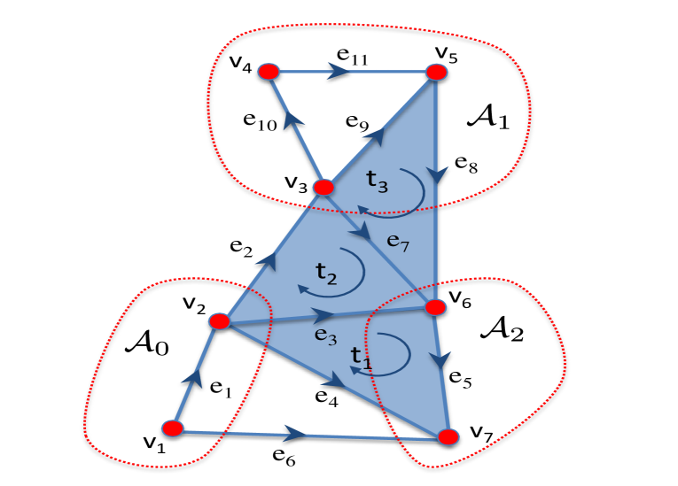
This operator maps the edge signal onto a signal defined over the triangle sets, i.e. in , and it is straightforward to verify that the generic -th entry of the is a measure of the flow circulating along the edges of the -th triangle. As an example for the simplicial complex in Fig. 1, we have
| (21) |
and, defining , we get . Each entry of is then the circulation over the corresponding triangle.
Similarly, the (discrete) divergence operator maps the edge signal onto a signal defined over the vertex space, i.e. , and it is defined as
| (22) |
Again, by direct substitution, it turns out that the -th entry of represents the net-flow passing through the -th vertex, i.e. the difference between the inflow and outflow at node . Thus a non-zero divergence reveals the presence of a source or sink node. For the example in Fig. 1, we get
| (23) |
so that .
If we consider equation (19) in the case ,
| (24) |
recalling that , it is easy to check that the first component in (24) has zero curl, and then it may be called an irrotational component, whereas the third component has zero divergence, and then it may be called a solenoidal component, in analogy to the calculus terminology used for vector fields. The harmonic component is a flow vector that is both curl-free and divergence-free. Notice also that, in (24), represents the (discrete) gradient of .
III-C Topology-aware unitary basis
In this section, we propose a method to build a unitary basis to represent edge signals, reflecting topological properties of the complex, more specifically triple-wise relations. The idea underlying the method is to search a basis that minimizes a real-valued function capturing triple-wise relations. For example, in the graph case, a key topological property is connectivity, which is well captured by the cut function. The associated real-valued function can be built using the so called Lovász extension [49], [50] of the cut size.
More specifically, given a graph and a partition of its vertex set in two sets and , with and , the cut size is defined as
| (25) |
where if and otherwise. is a set function and is known to be a submodular function [49]. Now, we want to translate the set function onto a real-valued function , defined over , to be used for the subsequent optimization. This can be done using the so called Lovász extension [49], which is equal to:
| (26) |
with . The function in (26) measures the total variation of a signal defined over the nodes of a graph and then it can be used as a regularization function, whenever the signal of interest is known to be a smooth function. The function in (26) formed the basis of the method proposed in [51] to build a unitary basis for analyzing signals defined over the vertices of a graph. More specifically, in [51] the basis was built by solving the following optimization problem
| (27) |
In the above problem, the objective function to be minimized is convex, but the problem is non-convex because of the unitarity constraint. To simplify the search for the basis, the objective function in (27) can be relaxed to become
| (28) |
Substituting (28) in (27), we still have a non-convex problem. However, its solution is known to be given by the eigenvectors of . From this perspective, the basis typically used in the GFT, built as the eigenvectors of the Laplacian matrix, can be interpreted as the solution of the above optimization problem, after relaxation.
Now, we extend the previous approach to find a regularization function capturing triple-wise relations, useful to analyze signals defined over the edges of a graph. In the previous case, the analysis of node signals started from the bi-partition of a graph and then the construction of a real-valued extension of the cut size. Here, to analyze edge signals, we need to start from the tri-partition of the discrete set and define a set function counting the number of triangles gluing the three sets together. The function to be minimized should then be the real valued (Lovász) extension of such a set function.
The combinatorial study of simplicial complexes has attracted increasing attention and the generalization of Cheeger inequalities to simplicial complexes has been the subject of several works [52], [53]. In particular, Hein et al. introduced the total variation on hypergraphs as the Lovász extension of the hypergraph cut, defined as the size of the hyperedges set connecting a bipartition of the vertex set [54]. In this work, we derive a Lovász extension defined over the edge set. More formally, we study a simplicial complex of order two, as in the example sketched in Fig.1, and consider the partition of in three sets . The triple-wise coupling function is now defined as
| (29) |
where if and otherwise. Our main result, stated in the following theorem, is that the Lovász extension of the triple-wise coupling function gives rise to a measure of the curl of edge signals along triangles.
Theorem 1
Proof:
Please see Appendix A. ∎
The function in (30) represents the sum of the absolute values of the curls over all the triangles. Differently from [54], where the total variation over a hypergraph was built from a bipartition of a discrete set and it was a function defined over , in our case, we start from a triparition of the original set and we build a real-valued extension, defined over , i.e. a space of dimension equal to the number of edges. A suitable unitary basis for representing (curling) edge signals can then be found as the solution of the following optimization problem
| (31) |
The objective function is convex, but the problem is non-convex because of the unitarity constraint. The above problem can be solved resorting to the algorithm proposed in [51], tuned to the new objective function given in (30). Alternatively, similarly to what is typically done with graphs, can be relaxed and replaced with
| (32) |
Substituting this function back to (31), the solution is given by the eigenvectors of .
The above arguments show that the eigenvectors of provide a suitable basis to analyze edge signals having a curling behavior. However, as we know from the Hodge decomposition recalled in the previous section, edge signals contain other useful components that are orthogonal to solenoidal signals, namely irrotational and harmonic components. Then, in general, it is useful to take as a unitary basis for analyzing edge signals all the eigenvectors of , i.e. the eigenvectors associated to the nonzero eigenvalues of and of , plus the eigenvectors associated to the kernel of . In summary, the theory developed in this section provides a further argument, rooted on intrinsic topological properties of the simplicial complex on which the signal is defined, to exploit the Hodge decomposition to find a suitable basis for the analysis of edge signals. Furthermore, the theory says that using the Laplacian eigenvectors comes as a consequence of a relaxation step. In many cases, whenever the numerical complexity is not an issue, it may be better to keep the -norm objective functions given in (26) and (30), as this would yield more sparse, and then more informative, representations, as a generalization of what done for directed graphs in [51].
IV Edge flows estimation
Let us consider now the observation of an edge signal affected by additive noise. Our goal in this section, is to formulate the denoising problem as a constrained problem, rooted on the Hodge decomposition. Denoising edge signals embedded in noise was already considered in [42],[31],[32] and, more specifically, in [18]. The formulation proposed in [18] was based on the definition of signals over simplicial complexes as skew-symmetric arrays of dimension equal to the order of the corresponding simplex plus one. So, the edge flow was represented as a matrix (i.e., a two-dimensional array) satisfying the constraint . A signal defined over the triangles was represented as an array of dimension three, satisfying the property . Our aim in this section, is to formulate the denoising optimization problem dealing only with vectors. Based on (19), the observed vector can be modeled as
| (33) |
where is noise. Let us suppose, for simplicity, that the noise vector is Gaussian, with zero-mean entries all having the same variance . The optimal estimator can then be formulated as the solution of the following problem
| (34) |
Note that problem is convex. Then, there exists multipliers such that the tuple satisfies the Karush-Kuhn-Tucker (KKT) conditions of (note that Slater’s constraint qualification is satisfied [55]). The associated Lagrangian function is
| (35) |
Exploiting the orthogonality property , it is easy to get the following KKT conditions
Note that conditions (a)-(c) reduce to
| (36) |
Multiplying both sides of condition (c) by , and using the second equality in (d) and condition (b), we get
| (37) |
This means that and may differ only by an additive vector lying in the nullspace of . Let us set , with . Similarly, multiplying (c) by and using the first equality in (d) and condition (a), we obtain
| (38) |
which implies that , with such that . Thus, condition (c) reduces to
| (39) |
which says, as expected, that we can derive the harmonic component by subtracting the estimated solenoidal and irrotational parts from the observed flow signal . To recover the irrotational flow from the -order signal we need to solve equation (a) in (36). Note that is not invertible. For connected graphs, it has rank and its kernel is the span of the vector of all ones. However, since the vector is also orthogonal to , the normal equation admits the nontrivial solution (at least for connected graphs):
where † denoted the Moore-Penrose pseudo-inverse.
Similarly, the -order signal , solution of the second equation in (36), can be obtained as
since is orthogonal to the null space of . The irrotational, solenoidal and harmonic components can then be recovered as follows
| (40) |
Note that the first two conditions in (36) imply that the variables , in are indeed decoupled so that the optimal solutions coincide with those of the following problems
| (41) |
| (42) |
(a)
(b)
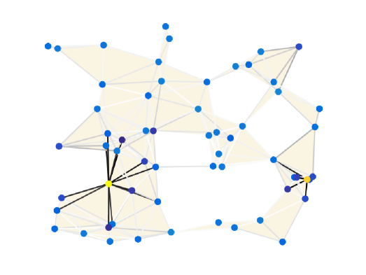
An example of an edge (flow) signal is reported in Fig. 2 (a), representing the simulation of data packet flow over a network, including measurement errors. The signal values are encoded in the gray color associated to each link. Suppose now, that the goal of processing is to detect nodes injecting anomalous traffic in the network, starting from the traffic shown in Fig. 2(a). If some node is a source of an anomalous traffic, that node generates an edge signal with a strong irrotational (or divergence-like) component. To detect spamming nodes, we can then project the overall observed traffic vector onto the space orthogonal to the space spanned by the nonzero eigenvectors of , computing
| (43) |
where is the matrix whose columns collect the eigenvectors associated with the nonzero eigenvalues of . The result of this projection is reported in Fig. 2(b), where we can clearly see that the only edges with a significant contributions are the ones located around two nodes, i.e. the source nodes injecting traffic in the network, whose divergence is encoded by the node color.
V Sampling and recovering of signal defined over simplicial complex
Suppose now that we only observe a few samples of a -order signal. The question we address here is to find the conditions to recover the whole signal from a subset of samples. To answer this question, we may use the theory developed in [56] for signals on graph, and later extended to hypergraphs in [57]. For simplicity, we focus on signals defined over a simplicial complex of order , i.e. on vertices, edges and triangles. Given a set of edges we define an edge-limiting operator as a diagonal matrix of dimension equal to the number of edges, with a one in the positions where we measure the flow, and zero elsewhere, i.e.
| (44) |
where is the set indicator vector whose -th entry is equal to one if the edge and zero otherwise. We say that an edge signal is perfectly localized over the subset (or -edge-limited) if . Similarly, given the matrix whose columns are the eigenvectors of , and a subset of indices , we define the operator
| (45) |
where . An edge signal is -bandlimited over a frequency set if . The operators and are self-adjoint and idempotent and represents orthogonal projectors, respectively, on the sets and . If we look for edges signals which are perfectly localized in both the edge and frequency domains, some conditions for perfect localization have been derived in [56]. More specifically: a) is perfectly localized over both the edge set and the frequency set if and only if the operator has an eigenvalue equal to one, i.e.
| (46) |
where denotes the spectral norm of ; b) a sufficient condition for the existence of such signals is that . Conversely, if , there could still exist perfectly localized vectors, when condition (46) holds.
In the following we first consider sampling on a single layer by extracting samples from the edge signals and then, we consider multi-layer processing using samples of signals defined over different layers of the simplex.
V-A Single-layer sampling
In the following theorem [56] we provide a necessary and sufficient condition to recover the edge signal from its samples .
Theorem 2
Given the bandlimited edge signal , it is possible to recover from a subset of samples collected over the subset if and only if the following condition holds:
| (47) |
with .
Proof:
The proof is a straightforward extension of Th. 4.1 in [56] to signals defined on the edges of the complex. ∎
In words, the above conditions mean that there can be no -bandlimited signals that are perfectly localized on the complementary set . Perfect recovery of the signal from can be achieved as
| (48) |
where . The existence of the above inverse is ensured by condition (47). In fact, the reconstruction error can be written as [56]
where we exploited in the second equality the bandlimited condition .
To make (47) holds true, we must guarantee that or, equivalently, that the matrix is full column rank, i.e. . Then, a necessary condition to ensure this holds is .
An alternative way to retrieve the overall signal from its samples can be obtained as follows.
If (47) holds true, the entire signal can be recovered from as follows
| (49) |
where is the matrix whose columns are the eigenvectors of associated with the frequency set .
Remark: It is worth to notice that, because of the Hodge decomposition (18), an edge signal always contains three components that are typically band-limited, as they reside on a subspace of dimension smaller than . This means that, if one knows a priori, that the edge signal contains only one component, e.g. solenoidal, irrotational, or harmonic, then it is possible to observe the edge signal and to recover the desired component over all the edges, under the conditions established by Theorem 2.
V-B Multi-layer sampling
In this section, we consider the case where we take samples of signals of different order and we propose two alternative strategies to retrieve an edge signal
from these samples.
The first approach aims at recovering
by using both, the vertex signal samples , with , and the edge samples . Hereinafter, we denote by , and
the set of frequency indexes in corresponding to the eigenvectors of belonging, respectively, to the irrotational, solenoidal and harmonic subspaces. Note that, if is -bandlimited then also , and are bandlimited with bandwidth, respectively, , and . Define
as the set of frequency indexes such that .
Furthermore, given the matrix with columns the eigenvectors of , we define the operator where denotes the bandwidth of .
Let be the set of indexes in associated with the eigenvectors belonging to and denote by the matrix whose columns are the eigenvectors of associated with the frequency set . Then, we can state the following theorem.
Theorem 3
Consider the second-order simplex and the edge signal . Then, assume that: i) the vertex-signal and the edge signal are bandlimited with bandwidth, respectively, and , where and denotes the number of eigenvectors in the bandwidth of belonging to ; ii) the conditions and hold true. Then, it follows that:
-
a)
can be perfectly recovered from both a set of vertex signal samples and from the edge samples via the set of equations
(50) where ,
(51) and ;
-
b)
There exists a set of frequency indexes , for which the eigenvectors matrix of satisfies the equality , and such that any -bandlimited edge signal with set of frequency indexes and can be recovered by using samples from and samples from .
Proof:
See Appendix B. ∎
Let us now consider the case where we want to recover from samples collected from signals of order , , and , i.e. , and . We denote by the vector of triangle signal samples with . Furthermore, given the matrix with columns the eigenvectors of the second-order Laplacian , we define the operator where denotes the bandwidth of . Then, assuming bandlimited, it holds . Denote with the set of indexes in associated with the eigenvectors belonging to and with the matrix whose columns are the eigenvectors of associated with the index set .
Theorem 4
Consider the second-order simplex , the edge signal and assume that: i) the vertex-signal , the edge signal and the triangle signal are bandlimited with bandwidth, respectively, , and , with and the number of eigenvectors in the bandwidth of and belonging, respectively, to and ; ii) all conditions , and hold true. Then, it follows:
-
a)
can be perfectly recovered from a set of vertex signal samples , from the edge samples and from the triangle samples as
(52) where
(53) and , , ;
-
b)
There exist two sets of frequency indexes , for which the eigenvectors of stacked in the columns of the matrices , satisfy, respectively, the equality , and . Then, any -bandlimited edge signal with frequency set , and , , can be recovered by using samples from , samples from and samples from .
Proof:
See Appendix B.∎
VI Estimation of discrete vector fields
Developing tools to process signals defined over simplicial complexes is also useful to devise algorithms for processing discrete vector fields. The use of algebraic topology, and more specifically Discrete Exterior Calculus (DEC), has been already considered for the analysis of vector fields, especially in the field of computer graphic. Exterior Calculus (EC) is a discipline that generalizes vector calculus to smooth manifolds of arbitrary dimensions [58] and DEC is a discretization of EC on simplicial complexes [59], [60]. DEC methodologies have been already proposed in [61] to produce smooth tangent vector fields in computer graphics. Smoothing tangential vector fields using techniques based on the spectral decomposition of higher order Laplacian was also advocated in [62].
In this section, building on the basic ideas of [61], [62], we propose an alternative approach to smooth discrete vector fields. More specifically, as in [61], [62], the proposed approach is based on three main steps: i) map the vector field onto an edge signal; ii) filter the edge signal; and iii) map the edge signal back to a vector field. Steps i) and iii) are essentially the same as in [62]. The difference we introduce here is in step ii), i.e. in the filtering of the edge signal. Filtering edge signals has been considered before, see, e.g., [32], but in our case we consider a different formulation and we incorporate the proper metrics in the Hodge Laplacian, dictated from the initial mapping from the vector field to the corresponding edge signal.
To filter vector fields, we need first to embed the vector field and the simplicial complex into a real space. Let us denote with a simplicial complex embedded in a real space of dimension . We assume that is flat, i.e. all simplices are in the same affine -subspace, and well-centered, which means the circumcenter of each simplex lies in its interior [59]. A discrete vector field can be considered as a map from points of to .
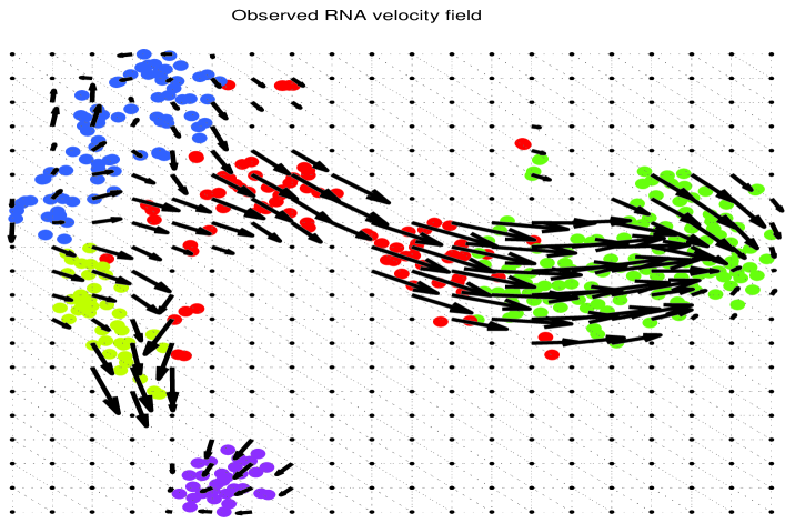
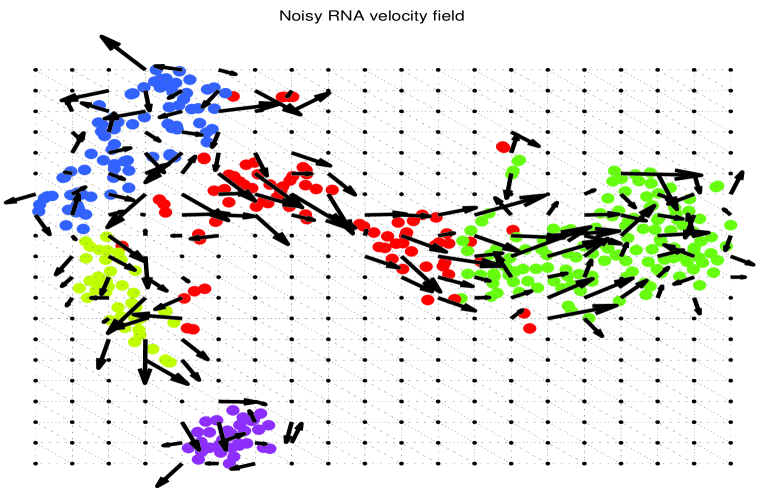
An illustrative example is shown in Fig. 3 (a), where the discrete vector field is represented by the set of arrows associated to the points in a regular grid in . In many applications, it is of interest to develop tools to extract relevant information from a vector field or to reduce the effect of noise.
Our proposed approach is based on the following three main steps:
1) Map a vector field onto a simplicial complex signal
Given the set of points , we build the simplicial complex using a well-centered Delaunay triangulation with vertices (-simplicies) in the points [59]. Then,
starting from the set of vectors ,
we recover a continuous vector field through interpolation based on the Whitney basis functions [63]
| (54) |
where are affine piecewise functions. More specifically, is an hat function on vertex , which takes on the value one at vertex , i.e. , is zero at all other vertices, and affine over each 2-simplex having as vertex. Then, project the vector field onto the set of -simplices (edges), giving rise to a set of scalar signals defined over the edges of the complex
| (55) |
where and are the end-points of edge and stands for the vector corresponding to , having the same direction as the orientation of . The vector of edge signals associated with the vector field , is then built as .
2) Filter the signal defined on the simplicial complex
The filtering strategy aims to recover an edge flow vector that fits the observed vector , it is smooth and sparse. We recover the vector as the solution of
where are positive penalty coefficients controlling, respectively, the signal smoothness and its sparsity. Since we chose the Whitney form as interpolation basis, for any two signals of order , , the induced inner product is given by , where the -dimensional matrix , incorporating the Whitney metric, is derived as in [60][Prop. 9.7]. Therefore, the Hodge Laplacian , weighted with the appropriate metric matrices , with , is a semidefinite positive matrix that can be written as
| (56) |
while the fitting error norm becomes
| (57) |
3) Map the filtered signal back onto a discrete vector field
Finally, given the discrete signal of order , , ,
the generated piecewise linear vector field becomes
[61]
| (58) |
(a)
(b)
(c)
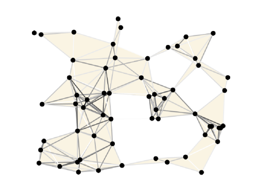
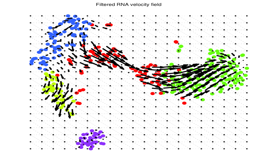
We show now an interesting application of the above procedure to the analysis of the vector field representing the RNA velocity field, defined as the time derivative of the gene expression state [41], useful to predict the future state of individual cells and then the direction of change of the entire transcriptome during the RNA sequencing dynamic process. The RNA velocity can be estimated by distinguishing between nascent (unspliced) and mature (spliced) messenger RNA (mRNA) in common single-cell RNA sequencing protocols [41]. We consider the mRNA-seq dataset of mouse chromaffin cell differentation analysed in [41]. An example of RNA velocity vector field is illustrated in Fig. 3(a). To analyze such a vector field using the proposed algorithms, we implemented steps 1) and 3) using the discrete exterior calculus operators provided by the PyDEC software developed in [60]. We considered a Delaunay well-centered triangulation of the continuous bi-dimensional space, which generates the simplicial complexes in Fig. 3 composed of nodes, where we fill all the triangles. The velocity field in Fig. 3(a) is observed over vertices and the field vector at each vertex has been obtained with a local Gaussian kernel smoothing [41]. The underlying colored cells represented different states of the cell differentiation process. Then, to test our filtering strategy, we added a strong Gaussian noise to the observed velocity field, with , as illustrated in Fig. 3(b). This noise is added to incorporate mRNA molecules degradation and model inaccuracy. Then we apply the proposed filtering strategy by first reconstructing the edge signal as in (54) and then recovering the edge signal as a solution of the optimization problem . Finally, we reconstruct the vector field using the interpolation formula (58), observed at the barycentric points of each triangles. The result is reported in Fig. 3(c), where we can appreciate the robustness of the proposed filtering strategy.
VII Inference of simplicial complex topology from data
The inference of the graph topology from (node) signals is a problem that has received significant attention, as shown in the recent tutorial papers [64], [39], [40] and in the references therein. In this section, we propose algorithms to infer the structure of a simplicial complex. Given the layer structure of a simplicial complex, we propose a hierarchical approach that infers the structure of one layer, assuming knowledge of the lower order layers. For simplicity, we focus on the inference of a complex of order from the observation of a set of edge (flow) signals , assuming that the topology of the underlying graph is given (or it has been estimated). So, we start from the knowledge of , which implies, after selection of an orientation, knowledge of . Since , then we need to estimate . Before doing that, we check, from the data, if the term is really needed. Since, from (24), the only components that may depend on are the solenoidal and harmonic components, we first project the observed flow signal onto the space orthogonal to the space spanned by the irrotational component, by computing
| (59) |
where is the matrix whose columns are the eigenvectors associated with the nonzero eigenvalues of . Then, denoting with the signal matrix of size , we measure the energy of by taking its norm : If the norm is smaller than a threshold of the averaged energy of the observed data set, we stop, otherwise we proceed to estimate .
The first step in the estimation of starts from the detection of all cliques of three elements present in the graph. Their number is . For each clique, we choose, arbitrarily, an orientation for the potential triangle filling it. The matrix can then be written as
| (60) |
where is the vector of size associated with the -th clique, whose entries are all zero except the three entries associated with the three edges of the -th clique. Those entries assume the value or , depending on the orientation of the triangle associated with the -th clique. The coefficients in (60) are equal to one, if there is a (filled) triangle on the -th clique, or zero otherwise. The goal of our inference algorithm is then to decide, starting from the data, which entries of are equal to one or zero. Our strategy is to make the association that enforces a small total variation of the observed flow signal on the inferred complex, using (32) as a measure of total variation on flow signals. We propose two alternative algorithms: The first method infers the structure of by minimizing the total variation of the observed data; the second method performs first a Principal Component Analysis (PCA) and then looks for the matrix and the coefficients of the expansion over the principal components that minimize the total variation plus a penalty on the model fitting error.
Minimum Total Variation (MTV) Algorithm: The goal of this algorithm is to minimize the total variation over the observed data set, assuming knowledge of the number of triangles. The set of coefficients is found as solution of
| (61) |
where is the number of triangles that we aim to detect. In practice, this number is not known, so it has to be found through cross-validation. Even though problem is non-convex, it can be solved in closed form. Introducing the nonnegative coefficients
, the solution can in fact be obtained by sorting the coefficients in increasing order and then selecting the triangles associated with the indices of
the lowest coefficients . Note that the proposed strategy infers the presence of triangles along the cliques having the minimum curl along its edges. Hence, we expect better performance when the edge signal contains only the harmonic components, whose curls along the filled triangles is exactly null.
PCA-based Best Fitting with Minimum Total Variation (PCA-BFMTV): To robustify the MTV algorithm in the case where the edge signal contains also a solenoidal component and is possibly corrupted by noise, we propose now the PCA-BFMTV algorithm that infers the structure of and the edge signal that best fits the observed data set , while at the same time exhibiting a small total variation over the inferred topology. The method starts performing a principal component analysis of the observed data by extracting the eigenvectors associated with the largest eigenvalues of the covariance matrix estimated from the observed data set. More specifically, the proposed strategy is composed of two steps: 1) estimate the covariance matrix from the edge signal data set and builds the matrix whose columns are the eigenvectors associated with the largest eigenvalues of ; 2) model the observed data set as and searches for the coefficient matrix and the vector that solve the following problem
| (62) |
where and is a non-negative coefficient controlling the trade-off between the data fitting error and the signal smoothness. Although problem is non-convex, it can be solved using an iterative alternating optimization algorithm returning successive estimates of , having fixed , and alternately , given . Interestingly, each step of the alternating optimization problem admits a closed form solution. More specifically, at each iteration , the coefficient matrix can be found as
Defining , problem admits the closed form solution
| (63) |
Then, given , we can find the vector using the same method used to solve problem MTV, in (61), i.e. setting and taking the entries of equal to for the indices corresponding to the first smallest coefficients of , and otherwise. The iterative steps of the proposed strategy are reported in the box entitled Algorithm PCA-BFMTV. Now we test the validity of our inference algorithms over both simulated and real data.
Set , , ,
,
Repeat
Set ;
Compute by sorting the coefficients
,
and setting to the entries of corresponding to the
smallest coefficients, and otherwise;
Set ,
until convergence.
Performance on synthetic data: Some of the most critical parameters affecting the goodness of the proposed algorithms are the dimension of the subspaces associated with the solenoidal and harmonic components of the signal and the number of filled triangles in the complex. In fact, in both MTV and PCA-BFMTV a key aspect is the detection of triangles as the cliques where the associated curl is minimum. Hence, if the signal contains only the harmonic component and there is no noise, the triangles can be identified with no error, because the harmonic component is null over the filled triangles. However, when there is a solenoidal component or noise, there might be decision errors.
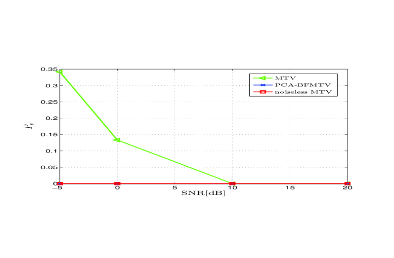
(a)
(b)
To test the inference capabilities of the proposed methods, in Fig. 4(a), we report the triangle error probability , defined as the percentage of incorrectly estimated triangles with respect to the number of cliques with three edges in the simplex, versus the signal-to-noise ratio (SNR), when the observation contains only harmonic flows plus noise. We considered a simplex composed of nodes and with a percentage of filled triangles with respect to the number of second order cliques in the graph equal to . We also set , and averaged our numerical results over zero-mean signal and noise random realizations. The harmonic signal bandwidth is chosen equal to , which is equal to the dimension of the kernel of . From Fig. 4(a), we can notice, as expected, that in the noiseless case the error probability is zero, since observing only harmonic flows enables perfect recovery of the matrix . In the presence of noise, the MTV algorithm suffers and in fact we observe a non negligible error probability at low SNR. However, applying the PCA-BFMTV algorithm enables a significant recovery of performance, as evidenced by the blue curve that is entirely superimposed to the red curve, at least for the SNR values shown in the figure. In this example, the covariance matrix was estimated over independent observations of the edge signals. The optimal coefficient was chosen after a cross validation operation following a line search approach aimed to minimize the error probability. The improvement of the PCA-BFMTV method with respect to the MTV method is due to the denoising made possible by the projection of the observed signal onto the space spanned by the eigenvectors associated with the largest eigenvalues of the estimated covariance matrix.
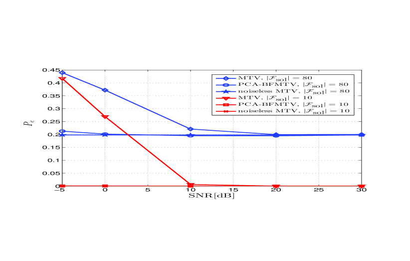
To test the proposed methods in the case where the observed signal contains both the solenoidal and harmonic components, in Fig. 4(b) we report versus the SNR, for different values of the dimension of the subspace associated with the solenoidal part, indicated as .
From Fig. 4(b), we can observe that the performance of both algorithms MTV and PCA-BFMTV suffers when the bandwidth of the solenoidal component is large, whereas the performance degradation becomes negligible when is small. In all cases, PCA-BFMTV significantly outperforms the MTV algorithm, especially at low SNR values, because of its superior noise attenuation capabilities. As further numerical test, we run algorithm replacing the quadratic regularization term with the triple-wise coupling regularization function in (30), by obtaining the same performance of the PCA-BFMTV algorithm.
Performance on real data: The real data set we used to test our algorithms is the set of mobile phone calls collected in the city of Milan, Italy, by Telecom Italia, in the context of the Telecom Big Data Challenge [65].
The data are associated with a regular two-dimensional grid, composed of points, superimposed to the city. Every point in the grid represents a square, of size meters. In particular, the data set collects the number of calls from node to area , as a function of time. There is an edge between nodes and only if there is a non null traffic between those points. The traffic has been aggregated in time, over time intervals of one hour. We define the flow signal over edge as . We map all the values of matrix into a vector of flow signals .
We observed the calls daily traffic during the month of December . The data are aggregated for each day over an interval of one hour.
Our first objective is to show whether there is an advantage in associating to the observed data set a complex of order , i.e. a set of triangles, or it is sufficient to use a purely graph-based approach. In both cases, we rely on the same graph structure, whose comes from the data set, after an arbitrary choice of the edges’ orientation. If we use a graph-based approach, we can build a basis of the observed flow signals using the eigenvectors of the so called edge Laplacian in [35], i.e. .
We call this basis . As an alternative, our proposed approach is to build a basis using the eigenvectors of , where is estimated from the data set using our MTV algorithm. We call this basis . To test the relative benefits of using as opposed to , we run a basis pursuit algorithm with the goal of finding a good trade-off between the sparsity of the representation and the fitting error. More specifically, for any given observed vector , we look for the sparse vector as solution of the following basis pursuit problem
[66]:
| (64) |
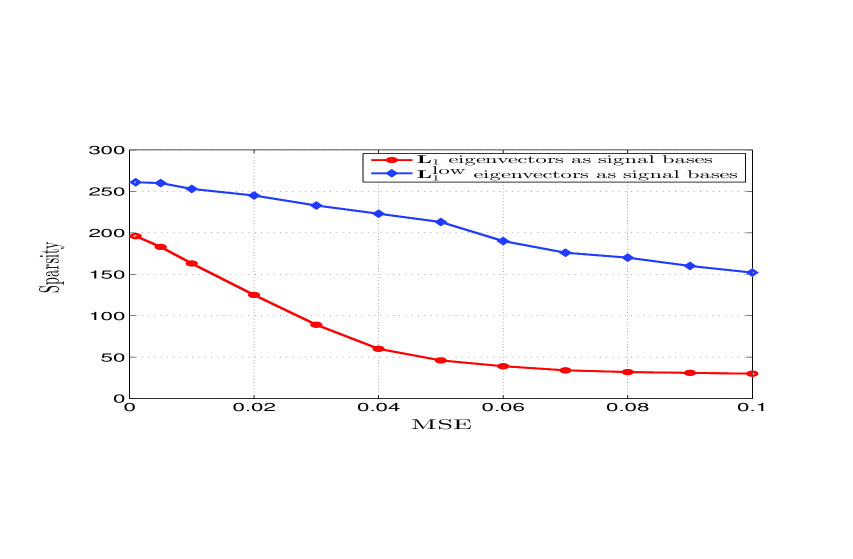
where in our case, while in the graph-based approach. As a numerical result, in Fig. 5 we report the sparsity of the recovered edge signals versus the mean estimation error considering as signal dictionary the eigenvectors of either the first-order Laplacian or the lower Laplacian. We used the MTV algorithm to infer the upper Laplacian matrix by setting the number of triangles that we may detect equal to . This value is derived numerically through cross-validation over a training data set, by choosing the value of that yields the minimum norm As can be observed from Fig. 5, using the set of the eigenvectors of yields a much smaller MSE, for a given sparsity or, conversely, a much more sparse representation, for a given MSE. An intuitive reason why our method performs so much better than a purely graph-based approach is that the matrix has a much reduced kernel space with respect to and the basis built on captures much better some inner structure present in the data by inferring the structure of the additional term from the data itself.
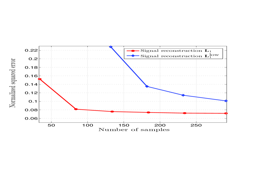
As a further test, we tested the two basis and in terms of the capability to recover the entire flow signal from a subset of samples. To this end, we exploit the band-limited property enforced by the sparse representation, enabling the use of the theory developed in Section V.A. Starting with the representation of each input vector as , with either in our case, or in the graph-based approach, we used the Max-Det greedy sampling strategy in [56] to select the subset of edges where to sample the flow signal and then we used the recovery rule in (49) to retrieve the overall flow signal from the samples. The numerical results are reported in Fig. 6, representing the normalized recovering error of the edge signal versus the number of samples used to reconstruct the overall signal. We can notice how introducing the term , we can achieve a much smaller error, for the same number of samples.
VIII Conclusion
In this paper we have presented an algebraic framework to analyze signals residing over a simplicial complex. In particular, we focused on signals defined over the edges of a complex of order two, i.e. including triangles, and we showed that exploiting the full algebraic structure of this complex provides an advantage with respect to graph-based tools only. We have not analyzed higher order signals. Nevertheless, looking at the structure of the higher order Laplacian and to the Hodge decomposition, the tools derived in this paper can be directly translated to analyze signals defined over higher order structures. What would be missing in the higher order cases would be a visual interpretation of the properties of the higher order Laplacian eigenvectors, as we could not be talking about solenoidal or irrotational behaviors.
We proposed a method to infer the structure of a second order simplicial complex from flow data and we showed that, in applications over real wireless traffic data, the proposed approach can significantly outperform methods based only on graph representations. Furthermore, we proposed a method to analyze discrete vector fields and showed an application to the recovery of the RNA velocity field to predict the evolution of living cells. In such a case, using the eigenvectors of we have been able to highlight irrotational and solenoidal behaviors that would have been difficult to highlight using only the eigenvectors of . Further developments should include both theoretical aspects, especially in the statistical modeling of random variables defined over a simplicial complex, and the generalization to higher order structures.
Appendix A Proof of Theorem 1
We begin by briefly recalling the basic properties of Lovász extension [49], [67] and then we proceed to the proof of Theorem 1.
Definition 1
Given a set , of cardinality , and its power set , let us consider a set function , with . Let be a vector of real variables, ordered w.l.o.g. in increasing order, such that . Define and for . Then, the Lovász extension of , evaluated at , is given by [49]:
| (65) |
An interesting property of set functions is submodularity, defined as follows:
Definition 2
A set function is submodular if and only if, , it satisfies the following inequality:
A fundamental property is that a set function is submodular iff its Lovász extension is a convex function and that minimizing on , is equivalent to minimizing the set function on [49, p.172]. Now, we wish to apply Lovász extension to a set function, defined over the edge set , counting the number of triangles gluing nodes belonging to a tri-partition of the node set . To this end, let us consider a tri-partition of the node set . Extending the approach used for graphs, where the cut-size is introduced as a set function evaluated on the node set, to define a triangle-cut size, we need to introduce a set function defined on the edge set. Given a simplex , assume the faces of to be positively oriented with the order of their vertices, i.e. for the -simplex we have with . Given any non-empty tri-partition of the node set , we define
| (66) |
as the set of triangles with exactly one vertex in each set , for . Given any , there exists a permutation of its vertices , , such that and , for . This returns a linear ordering111A binary relation on a set is a linear ordering on if it is transitive, antisymmetric and for any two elements , either or . of the vertices of the partition such that for all , if and , then precedes in the vertex ordering. Given the tri-partition , we define the set of oriented edges such that an oriented edge if and only if and for some . Thus, we can think of the triangle cut size in (29), equivalently, as a different function defined on sets of oriented edges, where denotes the complement set of in . Given an orientation on the simplicial complex, we can associate with the set of oriented edges the vector , whose entries are for edges in and for edges in , depending on the edge orientation. It is straightforward to check that , where is the edge-triangle incidence matrix defined in (3), computes the triangle cut for in the sense that each entry of this vector, corresponding to a triangle, is nonzero if and only if every vertex of that triangle is in a different set of the partition. As an example, considering the simplicial complex in Fig. 1, we have and the associated vector is . Then, using (21), we get and the triangle cut size is equal to .
Then, introducing the vector , we define the edge set function as
| (67) |
It can be proved that is invariant under any permutation of the vertexes of the triangles, since the effect of any vertex permutation is a change of sign in the entries of . Therefore, we get
| (68) |
Now we wish to derive the Lovász extension of the set function . Denote with the oriented -order simplex where , for . To make explicit the dependence of the function on the edge indexes , we rewrite (67) as
| (69) |
where, exploiting the structure of , given in (3), each term can be written as (we omit the dependence of on the edge set partition, for notation simplicity)
| (70) |
where , , are the entries of corresponding to the edge . is then a set function defined only on the power set of . We can now derive its Lovász extension . First, assume . Then, from Def. 1, we have , and . Therefore, from (70), it holds:
| (71) |
Then, from (65) we get:
Let us now assume . Thereby, we have , and , so that it results:
| (72) |
and
By following similar derivations, it is not difficult to show that for , , and , it holds . Therefore, from (69), defining the edge signal , we can write the Lovász extension of exploiting the additive property [49] as
| (73) |
or, equivalently, as
| (74) |
From the equality in (68), we can state that is the Lovász extension of . This completes the proof of Theorem .
References
- [1] S. Barbarossa, S. Sardellitti, and E. Ceci, “Learning from signals defined over simplicial complexes,” in 2018 IEEE Data Sci. Work. (DSW), 2018, pp. 51–55.
- [2] D. I. Shuman, S. K. Narang, P. Frossard, A. Ortega, and P. Vandergheynst, “The emerging field of signal processing on graphs: Extending high-dimensional data analysis to networks and other irregular domains,” IEEE Signal Process. Mag., vol. 30, no. 3, pp. 83–98, May 2013.
- [3] A. Ortega, P. Frossard, J. Kovačević, J. M. F. Moura, and P. Vandergheynst, “Graph signal processing: Overview, challenges, and applications,” Proc. of the IEEE, vol. 106, no. 5, pp. 808–828, May 2018.
- [4] S. Klamt, U.-U. Haus, and F. Theis, “Hypergraphs and cellular networks,” PLoS Comput. Biol., vol. 5, no. 5, 2009.
- [5] O. T. Courtney and G. Bianconi, “Generalized network structures: The configuration model and the canonical ensemble of simplicial complexes,” Phys. Rev. E, vol. 93, no. 6, pp. 062311, 2016.
- [6] C. Giusti, R. Ghrist, and D. S. Bassett, “Two’s company, three (or more) is a simplex,” J. Comput. Neurosci., vol. 41, no. 1, pp. 1–14, 2016.
- [7] T. Shen, Z. Zhang, Z. Chen, D. Gu, S. Liang, Y. Xu, R. Li, Y. Wei, Z. Liu, Y. Yi, and X. Xie, “A genome-scale metabolic network alignment method within a hypergraph-based framework using a rotational tensor-vector product,” Sci. Rep., vol. 8, no. 1, pp. 1–16, 2018.
- [8] A. R. Benson, R. Abebe, M. T. Schaub, A. Jadbabaie, and J. Kleinberg, “Simplicial closure and higher-order link prediction,” Proc. of Nat. Acad. of Sci., vol. 115, no. 48, pp. E11221–E11230, 2018.
- [9] S. Agarwal, K. Branson, and S. Belongie, “Higher order learning with graphs,” in Proc. 23rd Int. Conf. on Mach. Lear., 2006, pp. 17–24.
- [10] J. R. Munkres, Topology, Prentice Hall, 2000.
- [11] L. Kanari, P. Dłotko, M. Scolamiero, R. Levi, J. Shillcock, K. Hess, and H. Markram, “A topological representation of branching neuronal morphologies,” Neuroinfor., vol. 16, no. 1, pp. 3–13, 2018.
- [12] A. Patania, G. Petri, and F. Vaccarino, “The shape of collaborations,” EPJ Data Sci., vol. 6, no. 1, pp. 18, 2017.
- [13] R. Ramanathan, A. Bar-Noy, P. Basu, M. Johnson, W. Ren, A. Swami, and Q. Zhao, “Beyond graphs: Capturing groups in networks,” in Proc. IEEE Conf. Comp. Commun. Work. (INFOCOM), 2011, pp. 870–875.
- [14] T. J. Moore, R. J. Drost, P. Basu, R. Ramanathan, and A. Swami, “Analyzing collaboration networks using simplicial complexes: A case study,” in Proc. IEEE Conf. Comp. Commun. Work. (INFOCOM), 2012, pp. 238–243.
- [15] T. Roman, A. Nayyeri, B. T. Fasy, and R. Schwartz, “A simplicial complex-based approach to unmixing tumor progression data,” BMC Bioinfor., vol. 16, no. 1, pp. 254, 2015.
- [16] G. Carlsson, “Topology and data,” Bulletin Amer. Math. Soc., vol. 46, no. 2, pp. 255–308, 2009.
- [17] A. Muhammad and M. Egerstedt, “Control using higher order Laplacians in network topologies,” in Proc. of 17th Int. Symp. Math. Theory Netw. Syst., 2006, pp. 1024–1038.
- [18] X. Jiang, L. H. Lim, Y. Yao, and Y. Ye, “Statistical ranking and combinatorial Hodge theory,” Math. Program., vol. 127, no. 1, pp. 203–244, 2011.
- [19] Q. Xu, Q. Huang, T. Jiang, B. Yan, W. Lin, and Y. Yao, “HodgeRank on random graphs for subjective video quality assessment,” IEEE Trans. Multimedia, vol. 14, no. 3, pp. 844–857, June 2012.
- [20] A. Tahbaz-Salehi and A. Jadbabaie, “Distributed coverage verification in sensor networks without location information,” IEEE Trans. Autom. Contr., vol. 55, no. 8, pp. 1837–1849, Aug. 2010.
- [21] H. Chintakunta and H. Krim, “Distributed localization of coverage holes using topological persistence,” IEEE Trans. Signal Process., vol. 62, no. 10, pp. 2531–2541, May 2014.
- [22] V. De Silva and R. Ghrist, “Coverage in sensor networks via persistent homology,” Algeb. & Geom. Topol., vol. 7, no. 1, pp. 339–358, 2007.
- [23] S. Emrani, T. Gentimis, and H. Krim, “Persistent homology of delay embeddings and its application to wheeze detection,” IEEE Signal Process. Lett., vol. 21, no. 4, pp. 459–463, Apr. 2014.
- [24] H. Edelsbrunner and J. Harer, “Persistent homology-a survey,” Contemp. Math., vol. 453, pp. 257–282, 2008.
- [25] D. Horak, S. Maletić, and M. Rajković, “Persistent homology of complex networks,” J. Statis. Mech.: Theory and Experiment, vol. 2009, no. 3, pp. P03034, 2009.
- [26] H. Krim and A. B. Hamza, Geometric methods in signal and image analysis, Cambridge Univ. Press, 2015.
- [27] M. Robinson, Topological signal processing, Springer, 2016.
- [28] W. Huang, T. A. W. Bolton, J. D. Medaglia, D. S. Bassett, A. Ribeiro, and D. Van De Ville, “A graph signal processing perspective on functional brain imaging,” Proc. of the IEEE, vol. 106, no. 5, pp. 868–885, May 2018.
- [29] K. K. Leung, W. A. Massey, and W. Whitt, “Traffic models for wireless communication networks,” IEEE J. Sel. Areas Commun., vol. 12, no. 8, pp. 1353–1364, Oct. 1994.
- [30] R. Sever and J. S. Brugge, “Signal transduction in cancer,” Cold Spring Harbor Perspec. in Medic., vol. 5, no. 4: a006098, 2015.
- [31] M. T. Schaub and S. Segarra, “Flow smoothing and denoising: Graph signal processing in the edge-space,” in 2018 IEEE Global Conf. Signal Inf. Process. (GlobalSIP), Nov. 2018, pp. 735–739.
- [32] J. Jia, M. T. Schaub, S. Segarra, and A. R. Benson, “Graph-based semi-supervised & active learning for edge flows,” in Proc. of 25th ACM SIGKDD Int. Conf. Knowl. Disc. & Data Min., 2019, pp. 761–771.
- [33] T. S. Evans and R. Lambiotte, “Line graphs, link partitions, and overlapping communities,” Phys. Rev. E, vol. 80, Jul. 2009.
- [34] Y.-Y. Ahn, J. P. Bagrow, and S. Lehmann, “Link communities reveal multiscale complexity in networks,” Nature, vol. 466, pp. 761–764, 2010.
- [35] M. Mesbahi and M. Egerstedt, Graph theoretic methods in multiagent networks, vol. 33, Princ. Univ. Press, 2010.
- [36] S. Mukherjee and J. Steenbergen, “Random walks on simplicial complexes and harmonics,” Random Struct. & Algor., vol. 49, no. 2, pp. 379–405, 2016.
- [37] O. Parzanchevski and R. Rosenthal, “Simplicial complexes: spectrum, homology and random walks,” Random Struct. & Algor., vol. 50, no. 2, pp. 225–261, 2017.
- [38] M. T. Schaub, A. R. Benson, P. Horn, G. Lippner, and A. Jadbabaie, “Random walks on simplicial complexes and the normalized Hodge Laplacian,” arXiv preprint arXiv:1807.05044, 2018.
- [39] G. Mateos, S. Segarra, A. G. Marques, and A. Ribeiro, “Connecting the dots: Identifying network structure via graph signal processing,” IEEE Signal Process. Mag., vol. 36, no. 3, pp. 16–43, May 2019.
- [40] X. Dong, D. Thanou, M. Rabbat, and P. Frossard, “Learning graphs from data: A signal representation perspective,” IEEE Signal Process. Mag., vol. 36, no. 3, pp. 44–63, May 2019.
- [41] G. La Manno et al., “RNA velocity of single cells,” Nature, vol. 560, no. 7719, pp. 494–498, 2018.
- [42] L. J. Grady and J. R. Polimeni, Discrete calculus: Applied analysis on graphs for computational science, Sprin. Sci. & Busin. Media, 2010.
- [43] T. E. Goldberg, “Combinatorial Laplacians of simplicial complexes,” Senior Thesis, Bard College, 2002.
- [44] U. Von Luxburg, “A tutorial on spectral clustering,” Stat. Comput., vol. 17, no. 4, pp. 395–416, 2007.
- [45] D. Horak and J. Jost, “Spectra of combinatorial Laplace operators on simplicial complexes,” Adv. Math., vol. 244, pp. 303–336, 2013.
- [46] J. Steenbergen, Towards a spectral theory for simplicial complexes, Ph.D. thesis, Duke Univ., 2013.
- [47] L.-H. Lim, “Hodge Laplacians on graphs,” S. Mukherjee (Ed.), Geometry and Topology in Statistical Inference, Proc. Sympos. Appl. Math., 76, AMS, 2015.
- [48] B. Eckmann, “Harmonische funktionen und randwertaufgaben in einem komplex,” Comment. Math. Helv., vol. 17, no. 1, pp. 240–255, 1944.
- [49] F. Bach, Learning with Submodular Functions: A Convex Optimization Perspective, vol. 6, Foundations and Trends in Machine Learning, 2013.
- [50] L. Lovász, “Submodular functions and convexity,” in A. Bachem et al. (eds.) Math. Program. The State of the Art, Springer Berlin Heidelberg, pp. 235–257, 1983.
- [51] S. Sardellitti, S. Barbarossa, and P. Di Lorenzo, “On the graph Fourier transform for directed graphs,” IEEE J. Sel. Top. Signal Process., vol. 11, no. 6, pp. 796–811, Sept. 2017.
- [52] O. Parzanchevski, R. Rosenthal, and R. J. Tessler, “Isoperimetric inequalities in simplicial complexes,” Combinatorica, vol. 36, no. 2, pp. 195–227, 2016.
- [53] J. Steenbergen, C. Klivans, and S. Mukherjee, “A Cheeger-type inequality on simplicial complexes,” Adv. Appl. Math., vol. 56, pp. 56 –77, 2014.
- [54] M. Hein, S. Setzer, L. Jost, and S. S. Rangapuram, “The total variation on hypergraphs - Learning on hypergraphs revisited,” in Adv. Neur. Inform. Proces. Syst. (NIPS), Dec. 5-8 2013.
- [55] S. Boyd and L. Vandenberghe, Convex optimization, Cambridge university press, 2004.
- [56] M. Tsitsvero, S. Barbarossa, and P. Di Lorenzo, “Signals on graphs: Uncertainty principle and sampling,” IEEE Trans. Signal Process., vol. 64, no. 18, pp. 4845–4860, Sept. 2016.
- [57] S. Barbarossa and M. Tsitsvero, “An introduction to hypergraph signal processing,” in Proc. of IEEE Int. Conf. Acoust., Speech, Signal Process. (ICASSP), 2016, pp. 6425–6429.
- [58] Élie Cartan, “Sur certaines expressions différentielles et le problème de pfaff,” in Annales scientifiques de l’École Normale Supérieure, 1899, vol. 16, pp. 239–332.
- [59] A. N. Hirani, Discrete Exterior Calculus, PhD thesis, California Institute of Technology, May 2003.
- [60] N. Bell and A. N. Hirani, “Pydec: software and algorithms for discretization of exterior calculus,” ACM Trans. Math. Soft. (TOMS), vol. 39, no. 1, pp. 3, 2012.
- [61] M. Fisher, P. Schröder, M. Desbrun, and H. Hoppe, “Design of tangent vector fields,” in ACM Trans. Grap. (TOG), 2007, vol. 26, p. 56.
- [62] C. Brandt, L. Scandolo, E. Eisemann, and K. Hildebrandt, “Spectral processing of tangential vector fields,” in Computer Graphics Forum. Wiley Online Library, 2017, vol. 36, pp. 338–353.
- [63] J. Dodziuk, “Finite-difference approach to the Hodge theory of harmonic forms,” Amer. Jour. Math., vol. 98, no. 1, pp. 79–104, 1976.
- [64] G. B. Giannakis, Y. Shen, and G. V. Karanikolas, “Topology identification and learning over graphs: Accounting for nonlinearities and dynamics,” Proc. of the IEEE, vol. 106, no. 5, pp. 787–807, May 2018.
- [65] Big data-Dandelion API datasets, available at: https://dandelion.eu/.
- [66] S. S. Chen, D. L. Donoho, and M. A. Saunders, “Atomic decomposition by basis pursuit,” in SIAM J. Sci. Comput., 1998, vol. 20, pp. 33–61.
- [67] L. Jost, S. Setzer, and M. Hein, “Nonlinear eigenproblems in data analysis: Balanced graph cuts and the ratioDCA-Prox,” in Extrac. Quant. Infor. Complex Syst., Spr. Intern. Publ., vol. 102, pp. 263–279, 2014.
- [68] D. S. Bernstein, Matrix Mathematics: Theory, Facts, and Formulas with Application to Linear Systems Theory, Princeton Univ. Press, 2005.
Appendix B Supporting material
This document contains some supporting materials complementing the paper: “Topological Signal Processing over Simplicial Complexes” to appear in IEEE Transactions on Signal Processing. Section A contains Proposition , and its proof, that will be instrumental in proving Theorems and , respectively, in Sections B and C.
B-A Proposition 2
We need first to derive the relationship between the bandwidth of the edge signal and that of the vertex signal , as stated in the following proposition.
Proposition 2
Let be the irrotational part of with a -bandlimited vertex signal. Then, is a -bandlimited edge signal with the set of indexes of the eigenvectors of stacked in the columns of , such that . The bandwidth of is , where is the number of eigenvectors in the bandwidth of belonging to .
Proof:
Let us define the matrix whose columns , are the eigenvectors of the 0-order Laplacian . Since we get
| (75) |
where the last equality follows from the bandlimitedness of , i.e. . From the property 2) in Prop. 1, at each eigenvector of with corresponds an eigenvector of with the same eigenvalue. Let denote the matrix whose columns are the eigenvectors of associated to the frequency index set with
| (76) |
Then, if , we get
| (77) |
Therefore, equation (75) reduces to
| (78) |
From the equality , multiplying both sides by , we easily derive , so that equation (78) is equivalent to
| (79) |
Since , we can rewrite (79) as
| (80) |
This last equality proves that is a -bandlimited edge signal with as in (76) and bandwidth , defining . ∎
B-B Proof of Theorem 3
Given the sampled signals and , we get
| (81) |
with . Then, since it holds and , we easily obtain
| (82) |
where
| (83) |
with the set of frequency indexes in corresponding to the eigenvectors of belonging to the solenoidal and harmonic subspaces. Assuming that both the conditions and hold true, the matrix is invertible and from the inverse of partitioned matrices [68], we get
| (84) |
with . Then we can recovery the signals and as
| (85) |
This concludes the proof of point a). Let us prove next point b). From Proposition it results that, if is -bandlimited, then is a -bandlimted signal with given in (76). This implies that the edge signal is a -bandlimited edge signal with and bandwidth . Let us now consider the system in (85). We get
| (86) |
Using the first equation in (86) and the fact that , it holds
| (87) |
where the last equality follows from . Hence, from (87), it follows that to perfectly recover the solenoidal and harmonic parts of we need a number of samples at least equal to the signal bandwidth . Finally, from the first equation in (86) it follows that to perfectly recovering we need a number of samples at least equal to the bandwidth of the vertex signal . This concludes the proof of point b) in the theorem.
B-C Proof of Theorem 4
Given the sampled signals , and , we have
| (88) |
Then, using the bandlimitedness property, so that , and , we get
| (89) |
with
| (90) |
Under the assumptions , and , the matrix becomes invertible and from the inverse of partitioned matrices [68], we get
| (91) |
and , , . Then we can recovery the signals , and as
| (92) |
This concludes the proof of point a). Let us prove next point b). From Proposition 2, is a -bandlimited signal with given in (76). To find the bandwidth of the solenoidal part we can proceed in a similar way to the proof of Proposition 2. Using the bandlimitedness property of , so that , it results
| (93) |
with the matrix whose columns , are the eigenvectors of the second-order Laplacian . From Proposition 1 at each eigenvector with corresponds an eigenvector of with the same eigenvalue. Denote with the matrix whose columns are the eigenvectors of associated to the frequency index set with
| (94) |
Let us write as
where the columns of are the eigenvectors in the kernel of belonging to the bandwidth of . Therefore, it results
| (95) |
where we used the equality . Then equation (93) reduces to
| (96) |
Since it holds , , we easily get
| (97) |
Then is a -bandlimited edge signal with given in (94). This implies that is -bandlimited with and bandwidth . Let us now consider the system in (92). We get
| (98) |
Using equations in (98) and the fact that , it holds
| (99) |
Hence, from (99), it follows that to perfectly recover the harmonic part of we need a number of edge samples at least equal to the signal bandwidth . Finally, from the first and last equation in (98), we conclude that to retrieve and the solenoidal signal we need, respectively, a number of node samples and a number of triangle signal samples .