Topological susceptibility and axion properties in the presence of a strong magnetic field within the three-flavor NJL model

We consider a three-flavor NJL Lagrangian that includes scalar and pseudoscalar chiral quark couplings as well as a ’t Hooft six-fermion interaction term, in the presence of an external electromagnetic field ${\cal A}_{\mu}$. Moreover, we take into account the coupling to a field $\theta(x)=a(x)/f_{a}$ of the form given by Eq. (1). This can be effectively done through the ’t Hooft term (which accounts for the chiral U(1)_A anomaly) by performing a chiral rotation of quarks fields by an angle $\theta$. In this way, the effective Euclidean action is given by [27, 26]

$$S_{E}\ =\ \int d^{4}x\left\{\bar{\psi}\left(-i\ \hbox to0.0pt{/\hss}\!D+\hat{m}\right)\psi-G\sum_{a=0}^{8}\left[\left(\bar{\psi}\lambda_{a}\psi\right)^{2}+\left(\bar{\psi}\,i\gamma_{5}\lambda_{a}\psi\right)^{2}\right]+K\left(e^{i\theta}\,d_{+}+e^{-i\theta}\,d_{-}\right)\right\}\ ,$$

(3)

where $G$ and $K$ are coupling constants, $\psi=\left(\psi_{u},\psi_{d},\psi_{s}\right)^{T}$ stands for a quark three-flavor vector, $\hat{m}=\mathrm{diag}\left(m_{u},m_{d},m_{s}\right)$ is the corresponding current quark mass matrix, and $d_{\pm}=\det\left[\bar{\psi}\left(1\pm\gamma_{5}\right)\psi\right]$. In addition, $\lambda_{a}$ denote the Gell-Mann matrices, with $\lambda_{0}=\sqrt{2/3}\,I$, where $I$ is the unit matrix in the three flavor space. The coupling of quarks to the electromagnetic field is implemented through the covariant derivative $D_{\mu}=\partial_{\mu}-i\hat{Q}{\cal A}_{\mu}$, where $\hat{Q}=\mathrm{diag}\left(Q_{u},Q_{d},Q_{s}\right)$ represents the quark electric charge matrix, i.e. $Q_{u}/2=-Q_{d}=-Q_{s}=e/3$, $e$ being the proton electric charge. In the present work we consider a static and constant magnetic field in the $3$-direction.

We proceed by bosonizing the action in terms of scalar $\sigma_{a}(x)$ and pseudoscalar $\pi_{a}(x)$ fields, introducing also corresponding auxiliary $\mbox{s}_{a}(x)$ and $\mbox{p}_{a}(x)$ fields. Following a standard procedure, we start from the partition function

$$Z=\int D\bar{\psi}D\psi\ e^{-S_{E}}\,.$$

(4)

By introducing functional delta functions, the scalar ($\bar{\psi}\lambda_{a}\psi$) and pseudoscalar ($\bar{\psi}i\gamma_{5}\lambda_{a}\psi$) currents in $S_{E}$ can be replaced by $\mbox{s}_{a}(x)$ and $\mbox{p}_{a}(x)$, and one can perform the functional integration on the fermionic fields $\psi$ and $\bar{\psi}$. Then, to carry out the integration over the auxiliary fields we use the stationary phase approximation (SPA), keeping the functions $\tilde{\mbox{s}}_{a}(x)$ and $\tilde{\mbox{p}}_{a}(x)$ that minimize the integrand of the partition function. This yields a set of coupled equations among the bosonic fields, from which one can take $\tilde{\mbox{s}}_{a}(x)$ and $\tilde{\mbox{p}}_{a}(x)$ to be implicit functions of $\sigma_{a}(x)$ and $\pi_{a}(x)$. Finally, we consider the mean field (MF) approximation, expanding the bosonized action in powers of field fluctuations around the corresponding translationally invariant mean field values $\bar{\sigma}_{a}$ and $\bar{\pi}_{a}$. Thus, we write $\sigma_{a}(x)=\bar{\sigma}_{a}+\delta\sigma_{a}(x)$ and $\pi_{a}(x)=\bar{\pi}_{a}+\delta\pi_{a}(x)$, where, due to charge conservation, only $\bar{\sigma}_{a}$, $\bar{\pi}_{a}$ with $a=0,3,8$ can be nonzero. For convenience, we introduce the notation $\bar{\sigma}=\mathrm{diag}(\bar{\sigma}_{u},\bar{\sigma}_{d},\bar{\sigma}_{s})=\lambda_{0}\bar{\sigma}_{0}+\lambda_{3}\bar{\sigma}_{3}+\lambda_{8}\bar{\sigma}_{8}$ and $\bar{\pi}=\mathrm{diag}(\bar{\pi}_{u},\bar{\pi}_{d},\bar{\pi}_{s})=\lambda_{0}\bar{\pi}_{0}+\lambda_{3}\bar{\pi}_{3}+\lambda_{8}\bar{\pi}_{8}$.

At the mean field level, the Euclidean action per unit volume reads

	$\displaystyle\dfrac{\bar{S}_{\!E}^{\;\mathrm{bos}}}{V^{(4)}}\$	$\displaystyle=$	$\displaystyle-\dfrac{N_{c}}{V^{(4)}}\sum_{f}\int d^{4}x\,d^{4}x^{\prime}\ {\rm tr}_{D}\,\ln\left(\mathcal{S}^{f}_{x,x^{\prime}}\right)^{-1}-\dfrac{1}{2}\sum_{f}\Big{[}\,\bar{\sigma}_{f}\ \bar{\mbox{s}}_{f}+\bar{\pi}_{f}\ \bar{\mbox{p}}_{f}+G\left(\bar{\mbox{s}}_{f}^{2}+\bar{\mbox{p}}_{f}^{2}\right)\Big{]}$		(5)
			$\displaystyle+\ \frac{K}{4}\Big{[}\cos\theta\left(\bar{\mbox{s}}_{u}\bar{\mbox{s}}_{d}\bar{\mbox{s}}_{s}-\bar{\mbox{s}}_{u}\bar{\mbox{p}}_{d}\bar{\mbox{p}}_{s}-\bar{\mbox{p}}_{u}\bar{\mbox{s}}_{d}\bar{\mbox{p}}_{s}-\bar{\mbox{p}}_{u}\bar{\mbox{p}}_{d}\bar{\mbox{s}}_{s}\right)$
			$\displaystyle\qquad\quad-\sin\theta\left(\bar{\mbox{p}}_{u}\bar{\mbox{p}}_{d}\bar{\mbox{p}}_{s}-\bar{\mbox{p}}_{u}\bar{\mbox{s}}_{d}\bar{\mbox{s}}_{s}-\bar{\mbox{s}}_{u}\bar{\mbox{p}}_{d}\bar{\mbox{s}}_{s}-\bar{\mbox{s}}_{u}\bar{\mbox{s}}_{d}\bar{\mbox{p}}_{s}\right)\Big{]}\ ,$

where ${\rm tr}_{D}$ stands for trace in Dirac space, while

$$\left(\mathcal{S}^{f}_{x,x^{\prime}}\right)^{-1}\ =\ \delta(x-x^{\prime})\left[-i(\not{\partial}-iQ_{f}\not{\cal A})+M_{sf}+i\gamma_{5}\,M_{pf}\right]$$

(6)

is the inverse mean field quark propagator for each flavor. Here, we have used the definitions $M_{sf}=m_{f}+\bar{\sigma}_{f}$ and $M_{pf}=\bar{\pi}_{f}$. Moreover, in Eq. (5) $\bar{\mbox{s}}_{f}$ are the values of the auxiliary fields at the mean field level within the SPA approximation, i.e. $\bar{\mbox{s}}_{f}=\tilde{\mbox{s}}_{f}(\bar{\sigma}_{a})$. They satisfy the conditions

	$\displaystyle\bar{\sigma}_{i}+2G\,\bar{\mbox{s}}_{i}-\frac{K}{4}\,\sum_{jk}\,|\epsilon_{ijk}|\left[\left(\bar{\mbox{s}}_{j}\,\bar{\mbox{s}}_{k}-\bar{\mbox{p}}_{j}\ \bar{\mbox{p}}_{k}\right)\cos\theta+2\,\bar{\mbox{s}}_{j}\ \bar{\mbox{p}}_{k}\ \sin\theta\right]$	$\displaystyle=$	$\displaystyle 0\ ,$
	$\displaystyle\bar{\pi}_{i}+2G\,\bar{\mbox{p}}_{i}\,-\,\frac{K}{4}\,\sum_{jk}\,|\epsilon_{ijk}|\left[\left(\bar{\mbox{s}}_{j}\,\bar{\mbox{s}}_{k}-\bar{\mbox{p}}_{j}\ \bar{\mbox{p}}_{k}\right)\sin\theta-2\,\bar{\mbox{s}}_{j}\ \bar{\mbox{p}}_{k}\ \cos\theta\right]$	$\displaystyle=$	$\displaystyle 0\ ,$		(7)

where the values $1,2,3$ for indices $i$, $j$ and $k$ are equivalent to labels $f=u,d,s$. From the conditions $\delta\bar{S}_{\!E}^{\;\mathrm{bos}}/\delta\bar{\sigma}_{f}=0$ and $\delta\bar{S}_{\!E}^{\;\mathrm{bos}}/\delta\bar{\pi}_{f}=0$ one can get now the “gap equations”

$$\bar{\mbox{s}}_{f}\,=\,2\,\langle\bar{q}_{f}q_{f}\rangle\ ,\qquad\qquad\bar{\mbox{p}}_{f}\,=\,2\,\langle\bar{q}_{f}i\gamma_{5}q_{f}\rangle\ ,$$

(8)

where the quark-antiquark condensates are given by

$$\langle\bar{q}_{f}q_{f}\rangle\,=\,-\dfrac{N_{c}}{V^{(4)}}\int d^{4}x\ {\rm tr}_{D}\big{[}\mathcal{S}^{f}_{x,x}\big{]}\ ,\qquad\qquad\langle\bar{q}_{f}i\gamma_{5}q_{f}\rangle\,=\,-\dfrac{N_{c}}{V^{(4)}}\int d^{4}x\ {\rm tr}_{D}\big{[}i\gamma_{5}\,\mathcal{S}^{f}_{x,x}\big{]}\ .$$

(9)

As is well known, the quark propagator can be written in different ways. For convenience we use [28, 29]

$$\mathcal{S}^{f}_{x,x^{\prime}}\ =\ e^{i\Phi_{f}(x,x^{\prime})}\,\int\dfrac{d^{4}p}{(2\pi)^{4}}\ e^{ip\,(x-x^{\prime})}\,\tilde{\mathcal{S}}_{p}^{f}\,,$$

(10)

where $\Phi_{f}(x,x^{\prime})$ is the so-called Schwinger phase, which depends on the gauge choice, and vanishes for $x\rightarrow x^{\prime}$. We express $\tilde{\mathcal{S}}_{p}^{f}$ in the Landau level form

	$\displaystyle\!\!\!\!\!\!\!\!\!\tilde{\mathcal{S}}_{p}^{f}$	$\displaystyle=$	$\displaystyle 2\ e^{-\vec{p}^{\,2}_{\perp}/B_{f}}\ \sum_{k=0}^{\infty}\ \frac{(-1)^{k}}{M_{sf}^{2}+M_{pf}^{2}+p_{\parallel}^{2}+2kB_{f}}$		(11)
			$\displaystyle\!\!\!\!\!\!\!\!\!\!\!\!\!\times\left\{\left(M_{sf}-i\gamma_{5}\,M_{pf}-p_{\parallel}\cdot\gamma_{\parallel}\right)\left[\,\Gamma^{+}\,L_{k}\Big{(}\frac{2\vec{p}^{\,2}_{\perp}}{B_{f}}\Big{)}-\Gamma^{-}\,L_{k-1}\Big{(}\frac{2\vec{p}^{\,2}_{\perp}}{B_{f}}\Big{)}\right]+2\,\vec{p}_{\perp}\cdot\vec{\gamma}_{\perp}\,L^{1}_{k-1}\Big{(}\frac{2\vec{p}^{\,2}_{\perp}}{B_{f}}\Big{)}\right\}\ .$

Here, $L_{k}^{\alpha}(x)$ are generalized Laguerre polynomials, with the convention $L_{-1}^{\alpha}(x)=0$. We have also introduced the definitions $s_{f}={\rm sign}(Q_{f}B)$ and $B_{f}=|Q_{f}B|$, together with $\Gamma^{\pm}=(1\pm is_{f}\gamma_{1}\gamma_{2})/2$. “Perpendicular” and “parallel” gamma matrices have been collected into vectors $\gamma_{\perp}=(\gamma_{1},\gamma_{2})$ and $\gamma_{\parallel}=(\gamma_{3},\gamma_{4})$, and, in the same way, we have defined vectors $p_{\perp}=(p_{1},p_{2})$ and $p_{\parallel}=(p_{3},p_{4})$. Note that in our convention $\{\gamma_{\mu},\gamma_{\nu}\}=-2\delta_{\mu\nu}$.

The resulting expressions for $\bar{\mbox{s}}_{f}$ and $\bar{\mbox{p}}_{f}$ are divergent and have to be properly regularized. We use here the magnetic field independent regularization (MFIR) scheme, in which one subtracts from the unregulated integral the $B\to 0$ limit and then adds it in a regulated form. In this way, we obtain

$\displaystyle\bar{\mbox{s}}_{f}=-2N_{c}\,M_{sf}\,I_{1f}^{B}\ ,\qquad\qquad\bar{\mbox{p}}_{f}=-2N_{c}\,M_{pf}\,I_{1f}^{B}\ ,$

(12)

where

$\displaystyle I_{1f}^{B}\ =\ I_{1f}^{0}+I_{1f}^{\rm mag}\ .$

(13)

For the quantity $I_{1f}^{0}$ we use here a 3D cutoff regularization. Thus, we have

$$I^{0}_{1f}\ =\ \dfrac{1}{2\pi^{2}}\left[\Lambda\sqrt{\bar{M}_{f}^{2}+\Lambda^{2}}+\bar{M}_{f}^{2}\ \ln\left(\dfrac{\bar{M}_{f}}{\Lambda+\sqrt{\bar{M}_{f}^{2}+\Lambda^{2}}}\right)\right]\ ,$$

(14)

where $\bar{M}_{f}=\sqrt{M_{sf}^{2}+M_{pf}^{2}}\,$. On the other hand, the “magnetic piece” $I_{1f}^{\rm mag}$ is found to be given by

$$I_{1f}^{\rm mag}\ =\ \dfrac{B_{f}}{2\pi^{2}}\left[\ln\Gamma(x_{f})-\left(x_{f}-\dfrac{1}{2}\right)\ln x_{f}+x_{f}-\dfrac{\ln{2\pi}}{2}\right]\ ,$$

(15)

where $x_{f}=\bar{M}_{f}^{2}/(2B_{f})$.

The associated Euclidean regularized action per unit volume is given by

	$\displaystyle\dfrac{\bar{S}_{\!E}^{\;\mathrm{bos}}}{V^{(4)}}\,$	$\displaystyle=$	$\displaystyle\,\sum_{f}\,\omega_{f}^{B}-\dfrac{1}{2}\sum_{i}\,\left[\bar{\sigma}_{i}\ \bar{\mbox{s}}_{i}+\bar{\pi}_{i}\ \bar{\mbox{p}}_{i}+G\left(\bar{\mbox{s}}_{i}^{2}+\bar{\mbox{p}}_{i}^{2}\right)\right]$		(16)
			$\displaystyle+\;\frac{K}{24}\sum_{ijk}\,|\epsilon_{ijk}|\Big{[}\cos\theta\left(\bar{\mbox{s}}_{i}\bar{\mbox{s}}_{j}\bar{\mbox{s}}_{k}-3\,\bar{\mbox{s}}_{i}\bar{\mbox{p}}_{j}\bar{\mbox{p}}_{k}\right)-\sin\theta\left(\bar{\mbox{p}}_{i}\bar{\mbox{p}}_{j}\bar{\mbox{p}}_{k}-3\,\bar{\mbox{p}}_{i}\bar{\mbox{s}}_{j}\bar{\mbox{s}}_{k}\right)\Big{]}\ ,$

where

$\displaystyle\omega_{f}^{B}\ =\ \omega_{f}^{0}+\omega_{f}^{\rm mag}\ ,$

(17)

with

	$\displaystyle\omega_{f}^{0}$	$\displaystyle=$	$\displaystyle-\frac{N_{c}}{8\pi^{2}}\left[\Lambda\sqrt{\bar{M}_{f}^{2}+\Lambda^{2}}\left(\bar{M}_{f}^{2}+2\Lambda^{2}\right)+\bar{M}_{f}^{4}\ln\left(\frac{\bar{M}_{f}}{\Lambda+\sqrt{\bar{M}_{f}^{2}+\Lambda^{2}}}\right)\right]\ ,$		(18)
	$\displaystyle\omega_{f}^{\rm mag}$	$\displaystyle=$	$\displaystyle-\frac{N_{c}\,B_{f}^{2}}{2\pi^{2}}\left[\zeta^{\prime}(-1,x_{f})-\frac{x_{f}^{2}-x_{f}}{2}\ln x_{f}+\frac{x_{f}^{2}}{4}\right]\ .$		(19)

Here $\zeta^{\prime}(-1,x_{f})$ stands for the derivative of the Hurwitz zeta function.

Let us now consider the case of a system in equilibrium at a finite temperature $T$ and quark chemical potential $\mu$. We follow here a similar analysis as the one carried out in Ref. [26]. The expressions for the mean field values $\bar{s}_{f}$ and $\bar{p}_{f}$ can be written as in Eqs. (12), replacing the function $I_{1f}^{B}$ by

$\displaystyle I_{1f}^{B,T,\mu}\ =\ I_{1f}^{B}\,+\,I_{1f}^{{\rm mag},T,\mu}\ .$

(20)

where

$\displaystyle I_{1f}^{{\rm mag},T,\mu}\,$

$\displaystyle=$

$\displaystyle\,\frac{B_{f}}{4\pi^{2}}\sum_{k=0}^{\infty}\,\alpha_{k}\int_{-\infty}^{\infty}dp\ \frac{1}{E_{kpf}}\,\sum_{s=\pm}\,\frac{1}{1+\exp[(E_{kpf}+s\mu)/T]}\ ,$

(21)

with $\alpha_{k}=2-\delta_{k0}$, $E_{kpf}=\sqrt{p^{2}+2kB_{f}+\bar{M}_{f}^{2}}\,$.

In the same way, the associated regularized thermodynamical potential $\Omega$ can be expressed as in Eq. (16), replacing $\omega^{B}_{f}$ by $\omega_{f}^{B,T,\mu}$, where

$\displaystyle\omega_{f}^{B,T,\mu}\ =\ \omega_{f}^{B}\,+\,\omega_{f}^{{\rm mag},T,\mu}\ .$

(22)

The $T=0$, $\mu=0$ piece $\omega_{f}^{B}$ is given by Eqs. (17-19), while the finite $T,\mu$ piece reads

$$\omega_{f}^{{\rm mag},T,\mu}\ =\ -\frac{N_{c}\,T}{4\pi^{2}}\sum_{f}B_{f}\,\sum_{k=0}^{\infty}\,\alpha_{k}\int_{-\infty}^{\infty}dp\,\sum_{s=\pm}\,\ln\Big{\{}1+\exp[-(E_{kpf}+s\mu)/T]\Big{\}}\ .$$

(23)

As stated, the topological susceptibility $\chi_{t}$ is useful to analyze how the manifestations of the chiral anomaly are affected by the temperature and the external magnetic field. This quantity is given by

$$\chi_{t}\ =\ \int\ d^{4}x\,\langle 0|\,T\,Q(x)\,Q(0)|0\rangle\ ,$$

(24)

where $Q(x)$ is the topological charge

$$Q(x)\ =\ \frac{g^{2}}{32\pi^{2}}\;G_{\mu\nu}(x)\,\tilde{G}^{\mu\nu}(x)\ .$$

(25)

In the framework of the above introduced effective NJL model, $\chi_{t}$ can be simply calculated by taking the second derivative of the effective action with respect to $\theta$, viz.

$$\chi_{t}\ =\ \frac{d^{2}\Omega}{d\theta^{2}}\Big{|}_{\theta=0}\ .$$

(26)

The evaluation of the first derivative of $\Omega$ with respect to $\theta$ can be obtained taking into account the SPA equations

$$\frac{\partial\Omega}{\partial\bar{\mbox{s}}_{f}}\Big{|}_{s_{f}=\tilde{s}_{f}}\ =\ \frac{\partial\Omega}{\partial\bar{\mbox{p}}_{f}}\Big{|}_{s_{f}=\tilde{s}_{f}}\ =\ 0$$

(27)

together with the MF conditions

$$\frac{\partial\Omega}{\partial\sigma_{f}}\Big{|}_{\sigma_{f}=\bar{\sigma}_{f}}\ =\ \frac{\partial\Omega}{\partial\pi_{f}}\Big{|}_{\pi_{f}=\bar{\pi}_{f}}\ =\ 0\ .$$

(28)

Then, from Eq. (5) one has

$$\frac{d\Omega}{d\theta}\ =\ \frac{\partial\Omega}{\partial\theta}\ =\ -\frac{K}{24}\,\sum_{ijk}\,|\epsilon_{ijk}|\,\Big{[}\sin\theta\left(\bar{\mbox{s}}_{i}\bar{\mbox{s}}_{j}\bar{\mbox{s}}_{k}-3\,\bar{\mbox{s}}_{i}\bar{\mbox{p}}_{j}\bar{\mbox{p}}_{k}\right)+\cos\theta\left(\bar{\mbox{p}}_{i}\bar{\mbox{p}}_{j}\bar{\mbox{p}}_{k}-3\,\bar{\mbox{p}}_{i}\bar{\mbox{s}}_{j}\bar{\mbox{s}}_{k}\right)\Big{]}\ .$$

(29)

Using Eqs. (7), and noting that $\bar{\mbox{s}}_{f}\,M_{pf}=\bar{\mbox{p}}_{f}\,M_{sf}$ (see Eqs. (12)), one gets

$$\frac{d\Omega}{d\theta}\ =\ -\,\frac{1}{6}\sum_{f}\,m_{f}\,\bar{\mbox{p}}_{f}\ ,$$

(30)

where $m_{f}$ are the current quark masses. Moreover, it can be shown that the terms in the above sum over flavors are equal to each other. Indeed, from Eqs. (7) one has

	$\displaystyle m_{i}\,\bar{\mbox{p}}_{i}$	$\displaystyle\,=\,$	$\displaystyle\frac{K}{4}\,\sum_{jk}\,|\epsilon_{ijk}|\Big{[}\,\bar{\mbox{p}}_{i}\,\bar{\mbox{p}}_{j}\,\bar{\mbox{p}}_{k}\,\cos\theta\,+\,\bar{\mbox{s}}_{i}\,\bar{\mbox{s}}_{j}\,\bar{\mbox{s}}_{k}\sin\theta$		(31)
			$\displaystyle\,-\left(\bar{\mbox{p}}_{i}\,\bar{\mbox{s}}_{j}\,\bar{\mbox{s}}_{k}+2\,\bar{\mbox{s}}_{i}\,\bar{\mbox{p}}_{j}\,\bar{\mbox{s}}_{k}\right)\cos\theta\,-\,\left(\bar{\mbox{s}}_{i}\,\bar{\mbox{p}}_{j}\,\bar{\mbox{p}}_{k}+2\,\bar{\mbox{p}}_{i}\,\bar{\mbox{s}}_{j}\,\bar{\mbox{p}}_{k}\right)\sin\theta\,\Big{]}$
		$\displaystyle\,=\,$	$\displaystyle\frac{K}{12}\,\sum_{ljk}\,|\epsilon_{ljk}|\Big{[}\,\bar{\mbox{p}}_{l}\,\left(\bar{\mbox{p}}_{j}\,\bar{\mbox{p}}_{k}-3\bar{\mbox{s}}_{j}\,\bar{\mbox{s}}_{k}\right)\cos\theta\,+\,\bar{\mbox{s}}_{l}\,\left(\bar{\mbox{s}}_{j}\,\bar{\mbox{s}}_{k}-3\bar{\mbox{p}}_{j}\,\bar{\mbox{p}}_{k}\right)\sin\theta\,\Big{]}\ ,$

where the last expression does not depend on $i$. To derive this relation we have used the property

$$\sum_{jk}\,|\epsilon_{ijk}|\,(a_{i}\,b_{j}\,b_{k}+2\,b_{i}\,a_{j}\,b_{k})\ =\ \sum_{ljk}\,|\epsilon_{ljk}|\,a_{l}\,b_{j}\,b_{k}\ .$$

(32)

Thus, we have

$$\frac{d\Omega}{d\theta}\ =\ -\,\frac{1}{2}\;m_{f}\,\bar{\mbox{p}}_{f}\ ,$$

(33)

where $f$ can be either $u$, $d$ or $s$.

Notice that if any of the current quark masses (e.g. $m_{u}$) is taken to be equal to zero, one immediately obtains $d\Omega/d\theta=0$, i.e., the Lagrangian in Eq. (3) becomes independent of $\theta$. This is due to the existence of an additional U(1) global symmetry. In this limit the value of $\theta$ becomes unobservable, and, as is well known, the strong CP problem vanishes.

From the above equations it is easy to see that, as required by the Peccei-Quinn mechanism, the minimization condition $d\Omega/d\theta=0$ leads to the mean field values $\bar{\pi}_{f}=0$, $\bar{\theta}=0$. On the other hand, at the mean field level, the second derivative of the action with respect to $a=f_{a}\,\theta$ is nothing but the axion mass squared. Thus, the topological susceptibility and the axion mass are simply related by

$$f_{a}^{2}\,m_{a}^{2}\ =\ \frac{d^{2}\Omega}{d\theta^{2}}\Big{|}_{\theta=\bar{\theta}=0}\ =\ \chi_{t}\ .$$

(34)

To evaluate the second derivative in the above expression we need to determine $d\bar{\mbox{p}}_{f}/d\theta$. We have

$$\frac{d\bar{\mbox{p}}_{f}}{d\theta}\ =\ \frac{\partial\bar{\mbox{p}}_{f}}{\partial\bar{\sigma}_{f}}\,\frac{\partial\bar{\sigma}_{f}}{\partial\theta}\,+\,\frac{\partial\bar{\mbox{p}}_{f}}{\partial\bar{\pi}_{f}}\,\frac{\partial\bar{\pi}_{f}}{\partial\theta}\ .$$

(35)

The expressions for $\partial\bar{\mbox{p}}_{f}/\partial\bar{\sigma}_{f}$ and $\partial\bar{\mbox{p}}_{f}/\partial\bar{\pi}_{f}$ can be readily obtained from Eqs. (12) and the subsequent expressions of the functions $I_{1f}$ for zero and nonzero temperature. The partial derivatives of $\bar{\sigma}_{f}$ and $\bar{\pi}_{f}$ with respect to $\theta$ can be calculated by solving the coupled equations

	$\displaystyle\frac{\partial\bar{\sigma}_{i}}{\partial\theta}\,+\sum_{\phi=\bar{\sigma},\bar{\pi}}\bigg{[}2G\,\frac{\partial\bar{\mbox{s}}_{i}}{\partial\phi_{i}}\,\frac{\partial\phi_{i}}{\partial\theta}\,-\,\frac{K}{2}\,\sum_{jk}\,|\epsilon_{ijk}|\,\bigg{(}\frac{\partial\bar{\mbox{s}}_{j}}{\partial\phi_{j}}\,\bar{\mbox{s}}_{\theta,k}-\frac{\partial\bar{\mbox{p}}_{j}}{\partial\phi_{j}}\,\bar{\mbox{p}}_{\theta,k}\bigg{)}\frac{\partial\phi_{j}}{\partial\theta}\bigg{]}$	$\displaystyle\,=\,$	$\displaystyle-\,\bar{\pi}_{i}\,-\,2G\,\bar{\mbox{p}}_{i}\ ,$
	$\displaystyle\frac{\partial\bar{\pi}_{i}}{\partial\theta}\,+\sum_{\phi=\bar{\sigma},\bar{\pi}}\bigg{[}2G\,\frac{\partial\bar{\mbox{p}}_{i}}{\partial\phi_{i}}\,\frac{\partial\phi_{i}}{\partial\theta}\,+\,\frac{K}{2}\,\sum_{jk}\,|\epsilon_{ijk}|\,\bigg{(}\frac{\partial\bar{\mbox{s}}_{j}}{\partial\phi_{j}}\,\bar{\mbox{p}}_{\theta,k}+\frac{\partial\bar{\mbox{p}}_{j}}{\partial\phi_{j}}\,\bar{\mbox{s}}_{\theta,k}\bigg{)}\frac{\partial\phi_{j}}{\partial\theta}\bigg{]}$	$\displaystyle\,=\,$	$\displaystyle\bar{\sigma}_{i}\,+\,2G\,\bar{\mbox{s}}_{i}\ ,$		(36)

where we have introduced the shorthand notation

$$\bar{\mbox{s}}_{\theta,k}=\bar{\mbox{s}}_{k}\cos\theta+\bar{\mbox{p}}_{k}\sin\theta\ ,\qquad\qquad\bar{\mbox{p}}_{\theta,k}=\bar{\mbox{p}}_{k}\cos\theta-\bar{\mbox{s}}_{k}\sin\theta\ .$$

(37)

In the limit $\theta=0$ the equations get simplified, leading to the result

$$\chi_{t}\ =\ \frac{d^{2}\Omega}{d\theta^{2}}\Big{|}_{\theta=0}\ =\ -\frac{1}{2}\;\bigg{[}\,\frac{2}{K\,\bar{s}_{u}\,\bar{s}_{d}\,\bar{s}_{s}}\,+\,\sum_{k}\,\frac{1}{m_{k}\,\bar{s}_{k}}\,\bigg{]}^{-1}\ .$$

(38)

We recall that $\bar{s}_{f}$ is equal to twice the scalar condensate $\langle\bar{q}_{f}q_{f}\rangle$.

The expression in Eq. (38) can be compared to previous results obtained in the approximate chiral limit, where current masses are taken to be relatively small. At the lowest order in $m_{f}^{-1}$ one has

$$\chi_{t}\ \simeq\ -\frac{1}{2}\;\bigg{(}\,\sum_{k}\,\frac{1}{m_{k}\,\bar{s}_{k}}\,\bigg{)}^{-1}\ .$$

(39)

Moreover, assuming $\bar{s}_{u}\simeq\bar{s}_{d}\simeq\bar{s}_{s}$ one can approximate

$$\chi_{t}\ \simeq\ -\;\frac{\displaystyle\frac{1}{2}\,\sum_{k}\frac{\bar{s}_{k}}{m_{k}}}{\displaystyle\rule{0.0pt}{16.7871pt}\Big{(}\,\sum_{k}\,\frac{1}{m_{k}}\,\Big{)}^{2}}\ +\ {\cal O}\Big{(}\Delta_{su}^{2}\,,\Delta_{du}\Delta_{su}\,,\,\Delta_{du}^{2}\Big{)}\ ,$$

(40)

where $\Delta_{fu}=(\bar{s}_{f}-\bar{s}_{u})/\bar{s}_{u}$. This in agreement with the expressions found in Refs. [30, 22] and [31] in the contexts of ChPT and a linear sigma model, respectively. In the limit $\bar{s}_{u}=\bar{s}_{d}=\bar{s}_{s}$, the above expressions for $\chi_{t}$ reduce to the lowest-order ChPT Leutwyler-Smilga relation [32]

$$\chi_{t}\ \simeq\ -\;\frac{\bar{s}_{f}}{2}\,\Big{(}\,\sum_{k}\,\frac{1}{m_{k}}\,\Big{)}^{-1}\ .$$

(41)

Finally, it is also interesting to study the axion self-coupling arising from the $\theta$-dependent effective potential. It is usual to focus on the $\theta^{4}$ (i.e. $(a/f_{a})^{4}$) term in the effective action, defining the coupling parameter $\lambda_{a}$ as

$$\lambda_{a}\ =\ \frac{1}{f_{a}^{4}}\;\frac{d^{4}\Omega}{d\theta^{4}}\Big{|}_{\theta=0}\ .$$

(42)

Before presenting the numerical results for the topological susceptibility, we introduce the parameterization that has been chosen for the above discussed three-flavor version of the NJL model. Following Refs. [33, 34], we adopt the parameter set $m_{u}=m_{d}=5.5$ MeV, $m_{s}=140.7$ MeV, $\Lambda=602.3$ MeV, $G\Lambda^{2}=1.835$ and $K\Lambda^{5}=12.36$. This set has been determined in such a way that for $B=T=0$ one obtains meson masses $m_{\pi}=135$ MeV, $m_{K}=497.7$ MeV and $m_{\eta^{\prime}}=957.8$ MeV, together with a pion decay constant $f_{\pi}=92.4$ MeV.

It is well known that local NJL-like models fail to reproduce the inverse magnetic catalysis (IMC) effect at finite temperature. To address this issue, the possibility of allowing the coupling constant $G$ to depend on the magnetic field has been considered [35, 36, 37]. Taking into account the analysis carried out in Ref. [35], we consider a functional form

$\displaystyle G(B)\>=\>G\,\left[\dfrac{1+a\,(eB/\Lambda^{2}_{\rm QCD})^{2}+b\,(eB/\Lambda^{2}_{\rm QCD})^{3}}{1+c\,(eB/\Lambda^{2}_{\rm QCD})^{2}+d\,(eB/\Lambda^{2}_{\rm QCD})^{4}}\right]\ ,$

(43)

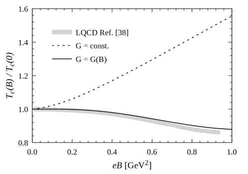
where the parameters $a$, $b$, $c$ and $d$ are determined by fitting the $B$ dependence of the pseudocritical chiral transition temperatures to those obtained through LQCD calculations [38]. The values of the parameters are [35] $a=0.0108805$, $b=-1.0133\times 10^{-4}$, $c=0.02228$ and $d=1.84558\times 10^{-4}$, with $\Lambda_{\rm QCD}=300$ MeV. The effect on the pseudocritical chiral restoration temperatures $T_{c}$ (at zero baryon chemical potential) is shown in Fig. 1, where we plot $T_{c}$ —normalized to $T_{c}(B=0)$— as a function of the magnetic field, considering the case of a constant coupling $G$ and the case in which one has a $B$-dependent coupling $G(B)$ as in Eq. (43) [35]. For comparison, the $B$ dependence of the normalized pseudocritical temperatures obtained from Lattice QCD calculations is also shown (gray band in the figure) [38]. The normalization temperature in our model is found to be $T_{c}(B=0)=173$ MeV, somewhat larger than the critical value obtained from LQCD calculations, $T_{c}(B=0)=156$ MeV [39].

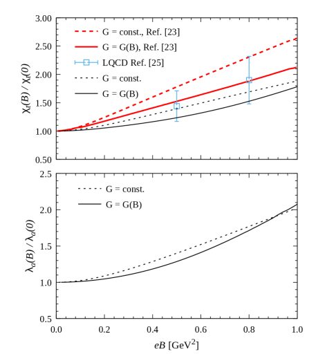
Let us start by quoting our numerical results for both zero quark chemical potential and zero temperature. In Fig. 2 we show the values of the topological susceptibility $\chi_{t}$ (upper panel) and the axion self-coupling parameter $\lambda_{a}$ (lower panel) as functions of the magnetic field, normalized by the corresponding values at $B=0$, namely $\chi_{t}(B=0)=78$ MeV and $\lambda_{a}(B=0)=0.85\times 10^{-5}$ GeV${}^{4}/f_{a}^{4}$. Black dashed and solid lines correspond to $G={\rm constant}$ and $G=G(B)$, respectively. It can be seen that in both cases $\chi_{t}$ and $\lambda_{a}$ show an enhancement with the magnetic field. Within errors, our results for the topological susceptibility are shown to be in agreement with those obtained from LQCD calculations (blue squares) [25] for a temperature $T\simeq 110$ MeV (which is well below the critical temperature, therefore the value of $\chi_{t}$ should be rather close to the one at $T=0$). In addition, we include for comparison the curves for $\chi_{t}$ corresponding to a two-flavor NJL model, taken from Ref. [23], both for constant and $B$-dependent couplings (red dashed and solid lines, respectively). The above mentioned value for $\chi_{t}$ at $B=0$ obtained within our model can be compared with the results obtained from ChPT [40] and LQCD [14] analyses, which lead to $\chi_{t}(B=0)\simeq 75.5$ MeV. In the case of the axion self-coupling, from ChPT the estimation $\lambda_{a}\simeq 1.12\times 10^{-5}$ GeV${}^{4}/f_{a}^{4}$ is obtained [41].

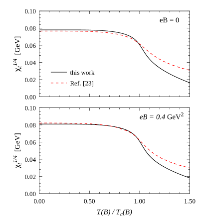
The behavior of the above quantities for nonzero temperatures is shown in Fig. 3, where we show the numerical results for $\chi_{t}^{1/4}$ and $\lambda_{a}\,f_{a}^{4}$ as functions of $T/T_{c}(B)$ for three representative values of the magnetic field. The pseudocritical chiral transition temperatures $T_{c}(B)$ have been defined taking the maximum values of the slopes $d\bar{s}_{l}/dT$, where $\bar{s}_{l}=(\bar{s}_{u}+\bar{s}_{d})/2$, for each value of the magnetic field. Left and right panels correspond to the results for constant and $B$-dependent couplings, respectively. As expected, one finds a sudden drop of both $\chi_{t}^{1/4}$ and $\lambda_{a}$ at $T=T_{c}$, signalling the restoration of chiral symmetry in the light quark sector. Notice that the curves for $\lambda_{a}$ tend to show a peak located at $T=T_{c}$.

In Fig. 4 we compare the results for $\chi_{t}^{1/4}$ obtained within our model, Eq. (38) (solid lines) with those arising from the approximate expressions in Eqs. (39) and (40) (dashed and dotted lines, respectively). The curves correspond to the case $G=G(B)$, for $eB=0$, 0.5 GeV² and 1 GeV². It can be seen that up to $T\simeq T_{c}$ all expressions are approximately equivalent for the considered values of the magnetic field. Beyond the chiral restoration transition, the curves corresponding to the approximate expressions in Eqs. (39) and (40) show some deviation with respect to the full result in Eq. (38). This difference is mainly due to the fact that the first term into the brackets, on the right hand side of Eq. (38), becomes nonnegligible in this region.

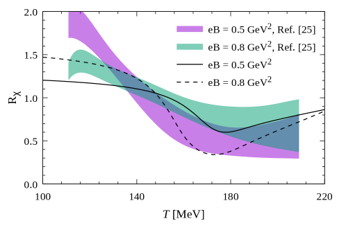
Our numerical results for the temperature dependence of $\chi_{t}$ can also be compared with those recently obtained from LQCD calculations, see Ref. [25]. To perform the comparison we consider the normalized quantity $R_{\chi}\equiv\chi_{t}(B,T)/\chi_{t}(0,T)$ introduced in that work. In Fig. 5 we show our results (black curves) together with those quoted in Ref. [25] (shaded bands) for $eB=0.5$ and 0.8 GeV². We include in the figure just the curves that correspond to the case of the $B$-dependent coupling $G(B)$, which, as stated, is the one consistent with LQCD results for IMC. Once again, it is seen that the predictions of the NJL model show qualitative agreement with LQCD calculations.

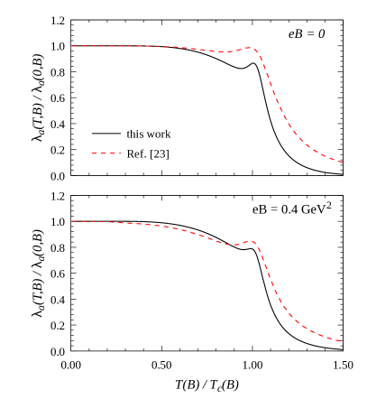
In Fig. 6 we go back to our results for $\chi_{t}^{1/4}$ and $\lambda_{a}$ as functions of the temperature, this time normalizing $\lambda_{a}$ to the corresponding value at $T=0$ and taking the magnetic field values $eB=0$ and $eB=0.4$ GeV², in order to compare our results (black solid lines) with those obtained within the two-flavor NJL model studied in Ref. [23] (red dashed lines). As in Fig. 5, our results correspond to $G=G(B)$, given by Eq. (43). The values of the temperature have been normalized to the critical temperatures $T_{c}(B)$, which are somewhat different for both models. This is in part due to the fact that in Ref. [23] an explicit dependence on both $B$ and $T$ has been assumed for the coupling $G$. It is seen that for the two-flavor model the peak of $\lambda_{a}$ at $T=T_{c}$ is slightly higher, while the fall of both $\chi_{t}^{1/4}$ and $\lambda_{a}$ for $T>T_{c}$ is less pronounced than in the case of the three-flavor NJL model. Nonetheless, it could be said that the behavior of $\chi_{t}^{1/4}$ and $\lambda_{a}$ is found to be qualitatively similar for both models.

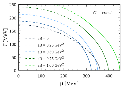
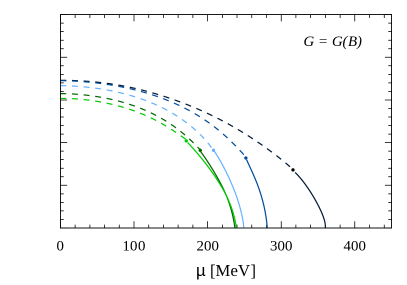
We turn now to discuss our numerical results for systems at nonzero quark chemical potential $\mu$. For a better comprehension, we start by briefly reviewing the phase diagrams in the $\mu-T$ plane, shown in Fig. 7. As expected, for low temperatures the system undergoes a first order chiral restoration transition at given critical chemical potentials $\mu_{c}(B,T)$. In the figure we show the corresponding transition lines (solid lines in the figure) for some representative values of the magnetic field. These first order transition lines finish at some critical end points (CEPs), whose positions depend on the external magnetic field. For higher values of the temperature, the transitions turn into smooth crossovers (dashed lines in the figure), as discussed for the systems at $\mu=0$.

Left and right panels of Fig. 7 correspond to constant and $B$-dependent $G$, respectively. As stated, the assumption of a $B$ dependence as the one in Eq. (43) leads to IMC, implying a significant change in the phase diagrams with respect to those obtained for the $G={\rm constant}$ case. On the other hand, the behavior of the CEP with the magnetic field is known to be strongly model-dependent. It is seen that our results for the case $G=G(B)$ are found to be qualitatively similar to those obtained in Ref. [42], where a three-flavor Polyakov-NJL model with a $B$-dependent coupling is studied; however, the behavior of the CEP is shown to be different from the one found in Ref. [43], where a nonlocal NJL-like model is considered (notice that in this type of model IMC is naturally obtained [44, 45]).

In Fig. 8 we show the behavior of $\chi_{t}^{1/4}$ as a function of the temperature, taking some representative values of the chemical potential and the magnetic field. The curves show clearly the first order and crossover transitions, both for the cases of $G={\rm constant}$ (left panels) and $G=G(B)$ (right panels). We have also verified that for nonzero $\mu$ the expressions in Eqs. (39) and (40) still approximate with good accuracy ($\lesssim 1$%) the exact result in Eq. (38), for temperatures that lie below the chiral transition. Then, in Fig. 9 we show the behavior of the axion self-coupling $\lambda_{a}$ (times the dimensionful scale $f_{a}^{4}$), for the same values of $\mu$ and $eB$. It is seen that the peak in $\lambda_{a}$ —which at $\mu=0$ was found to occur at the pseudocritical temperature— goes to infinity when the transition reaches the CEP, and turns into a first order transition jump beyond the CEP. This shows that at the transition the coupling $\lambda_{a}$ behaves like the derivative of an order parameter, and the position of the peak could be used to define the pseudocritical transition temperature related with the restoration of the U(1)_A symmetry.

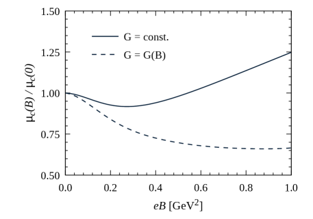
To conclude this section, we discuss the numerical results obtained for zero temperature and finite quark chemical potential. In Fig. 10 we show the behavior of the critical chemical potential $\mu_{c}(B,0)$ as a function of the magnetic field, both for constant and $B$-dependent couplings. The values are normalized to $\mu_{c}(0,0)$. It is interesting to notice that for $B\lesssim 0.3$ GeV² the models show again an IMC-like effect, i.e., a decrease of the critical chemical potential for increasing values of the magnetic field. This effect has been observed in various effective approaches to low energy QCD, including local and nonlocal NJL-like models [46, 47, 48, 49, 50]. For $G=G(B)$ it is seen that the IMC extends to larger values of the magnetic field, while for constant $G$ the values of $\mu_{c}$ reach a minimum and then get increased. This growth is consistent with the results in Ref. [48], where a constant value of $G$ is assumed, while the persistent IMC behavior is similar to the one obtained in nonlocal NJL models [50], where nonlocality leads to an effective dependence of the couplings on the magnetic field [45].

In Fig. 11 we show the behavior of $\chi_{t}^{1/4}$ and $\lambda_{a}/\lambda_{a}(\mu=0,B=0)$ as functions of the chemical potential, for three representative values of $eB$. Left and right panels correspond to constant and $B$-dependent couplings, respectively. The first order chiral transitions can be clearly observed. Moreover, it can be seen that beyond these transitions there is a second discontinuity, which corresponds to the partial chiral symmetry restoration related to the $s$ quark-antiquark condensate. Finally, in Fig. 12 we show the behavior of $\chi_{t}^{1/4}$ and $\lambda_{a}/\lambda_{a}(\mu=0,B=0)$ as functions of the magnetic field, for some selected values of $\mu$. Here we use a logarithmic scale, in order to focus on the region of low $eB$, and we just include the results for $G=G(B)$ (the curves for $G={\rm constant}$ are similar for values of $eB$ up to about 0.3 GeV²). As one can see from Fig. 10, for low values of $\mu$ the system lies in the chiral symmetry broken phase for all considered values of $eB$. Then, for $\mu\gtrsim 230$ MeV a first order transition is found at some intermediate value of $eB$, while for values of $\mu$ beyond $\mu_{c}(0,0)=359$ MeV the system lies in the partially restored chiral symmetry phase. Typically, in this region one finds for $T=0$ a series of magnetic oscillations related to the van Alphen-de Haas effect [51]. In fact, as shown in the figure, one finds a sequence of first order transitions that correspond to the values of $\mu$ that satisfy the relation $\mu^{2}=2kB_{f}+\bar{M}_{f}^{2}$ ($f=u,d$) for integer $k$. The value of $\chi_{t}^{1/4}$ is found to be relatively large for $\mu$ right above $\mu_{c}$ at low values of the magnetic field, and becomes significantly reduced when $eB$ is increased up to $\sim 1$ GeV².

References

- [1] A. A. Belavin, A. M. Polyakov, A. S. Schwartz and Y. S. Tyupkin, Phys. Lett. B 59, 85-87 (1975).
- [2] C. G. Callan, Jr., R. F. Dashen and D. J. Gross, Phys. Lett. B 63, 334-340 (1976).
- [3] R. D. Peccei and H. R. Quinn, Phys. Rev. Lett. 38, 1440-1443 (1977).
- [4] R. D. Peccei, Lect. Notes Phys. 741, 3-17 (2008) [arXiv:hep-ph/0607268 [hep-ph]].
- [5] L. Di Luzio, M. Giannotti, E. Nardi and L. Visinelli, Phys. Rept. 870, 1-117 (2020) [arXiv:2003.01100 [hep-ph]].
- [6] J. Preskill, M. B. Wise and F. Wilczek, Phys. Lett. B 120, 127-132 (1983).
- [7] L. F. Abbott and P. Sikivie, Phys. Lett. B 120, 133-136 (1983).
- [8] M. Dine and W. Fischler, Phys. Lett. B 120, 137-141 (1983).
- [9] G. G. Raffelt, Lect. Notes Phys. 741, 51-71 (2008) [arXiv:hep-ph/0611350 [hep-ph]].
- [10] A. Sedrakian, Phys. Rev. D 93, no.6, 065044 (2016) [arXiv:1512.07828 [astro-ph.HE]].
- [11] K. Fukushima, K. Ohnishi and K. Ohta, Phys. Rev. C 63, 045203 (2001) [arXiv:nucl-th/0101062 [nucl-th]].
- [12] P. Costa, M. C. Ruivo, C. A. de Sousa, H. Hansen and W. M. Alberico, Phys. Rev. D 79, 116003 (2009) [arXiv:0807.2134 [hep-ph]].
- [13] G. A. Contrera, D. G. Dumm and N. N. Scoccola, Phys. Rev. D 81, 054005 (2010) [arXiv:0911.3848 [hep-ph]].
- [14] S. Borsanyi, Z. Fodor, J. Guenther, K. H. Kampert, S. D. Katz, T. Kawanai, T. G. Kovacs, S. W. Mages, A. Pasztor and F. Pittler, et al. Nature 539, no.7627, 69-71 (2016) [arXiv:1606.07494 [hep-lat]].
- [15] P. Petreczky, H. P. Schadler and S. Sharma, Phys. Lett. B 762, 498-505 (2016) [arXiv:1606.03145 [hep-lat]].
- [16] Y. Taniguchi, K. Kanaya, H. Suzuki and T. Umeda, Phys. Rev. D 95, no.5, 054502 (2017) [arXiv:1611.02411 [hep-lat]].
- [17] K. Fukushima, D. E. Kharzeev and H. J. Warringa, Phys. Rev. D 78, 074033 (2008) [arXiv:0808.3382 [hep-ph]].
- [18] D. E. Kharzeev, J. Liao and P. Tribedy, [arXiv:2405.05427 [nucl-th]].
- [19] M. Asakawa, A. Majumder and B. Muller, Phys. Rev. C 81, 064912 (2010) [arXiv:1003.2436 [hep-ph]].
- [20] P. Adhikari, Phys. Lett. B 825, 136826 (2022) [arXiv:2103.05048 [hep-ph]].
- [21] P. Adhikari, Nucl. Phys. B 974, 115627 (2022) [arXiv:2111.06196 [hep-ph]].
- [22] P. Adhikari, Nucl. Phys. B 982, 115853 (2022) [arXiv:2203.00200 [hep-ph]].
- [23] A. Bandyopadhyay, R. L. S. Farias, B. S. Lopes and R. O. Ramos, Phys. Rev. D 100, no.7, 076021 (2019) arXiv:1906.09250 [hep-ph]].
- [24] M. S. Ali, C. A. Islam and R. Sharma, Phys. Rev. D 104, no.11, 114026 (2021) [arXiv:2009.13563 [hep-ph]].
- [25] B. B. Brandt, G. Endrődi, J. J. H. Hernández and G. Markó, [arXiv:2409.00796 [hep-lat]].
- [26] B. Chatterjee, H. Mishra and A. Mishra, Phys. Rev. D 91, no.3, 034031 (2015) [arXiv:1409.3454 [hep-ph]].
- [27] J. K. Boomsma and D. Boer, Phys. Rev. D 80, 034019 (2009) [arXiv:0905.4660 [hep-ph]].
- [28] V. A. Miransky and I. A. Shovkovy, Phys. Rept. 576, 1-209 (2015) [arXiv:1503.00732 [hep-ph]].
- [29] J. O. Andersen, W. R. Naylor and A. Tranberg, Rev. Mod. Phys. 88, 025001 (2016) [arXiv:1411.7176 [hep-ph]].
- [30] Y. Y. Mao et al. [TWQCD], Phys. Rev. D 80, 034502 (2009) [arXiv:0903.2146 [hep-lat]].
- [31] M. Kawaguchi, S. Matsuzaki and A. Tomiya, Phys. Rev. D 103, no.5, 054034 (2021) [arXiv:2005.07003 [hep-ph]].
- [32] H. Leutwyler and A. V. Smilga, Phys. Rev. D 46, 5607-5632 (1992).
- [33] P. Rehberg, S. P. Klevansky and J. Hufner, Phys. Rev. C 53 (1996), 410-429 [arXiv:hep-ph/9506436 [hep-ph]].
- [34] M. Coppola, W. R. Tavares, S. S. Avancini, J. C. Sodré and N. N. Scoccola, [arXiv:2410.05568 [hep-ph]].
- [35] M. Ferreira, P. Costa, O. Lourenço, T. Frederico and C. Providência, Phys. Rev. D 89 (2014) no.11, 116011 [arXiv:1404.5577 [hep-ph]].
- [36] R. L. S. Farias, K. P. Gomes, G. I. Krein and M. B. Pinto, Phys. Rev. C 90 (2014) no.2, 025203 [arXiv:1404.3931 [hep-ph]].
- [37] R. L. S. Farias, V. S. Timoteo, S. S. Avancini, M. B. Pinto and G. Krein, Eur. Phys. J. A 53 (2017) no.5, 101 [arXiv:1603.03847 [hep-ph]].
- [38] G. S. Bali, F. Bruckmann, G. Endrodi, Z. Fodor, S. D. Katz, S. Krieg, A. Schafer and K. K. Szabo, JHEP 02 (2012), 044 [arXiv:1111.4956 [hep-lat]].
- [39] A. Bazavov et al. [HotQCD], Phys. Lett. B 795, 15-21 (2019) [arXiv:1812.08235 [hep-lat]].
- [40] M. Gorghetto and G. Villadoro, JHEP 03, 033 (2019) [arXiv:1812.01008 [hep-ph]].
- [41] G. Grilli di Cortona, E. Hardy, J. Pardo Vega and G. Villadoro, JHEP 01, 034 (2016) [arXiv:1511.02867 [hep-ph]].
- [42] P. Costa, M. Ferreira, D. P. Menezes, J. Moreira and C. Providência, Phys. Rev. D 92, no.3, 036012 (2015) [arXiv:1508.07870 [hep-ph]].
- [43] J. P. Carlomagno, S. A. Ferraris, D. Gomez Dumm and A. G. Grunfeld, Phys. Rev. D 108, no.5, 056029 (2023) [arXiv:2305.15540 [hep-ph]].
- [44] V. P. Pagura, D. Gomez Dumm, S. Noguera and N. N. Scoccola, Phys. Rev. D 95, no.3, 034013 (2017) [arXiv:1609.02025 [hep-ph]].
- [45] D. Gómez Dumm, M. F. Izzo Villafañe, S. Noguera, V. P. Pagura and N. N. Scoccola, Phys. Rev. D 96, no.11, 114012 (2017) [arXiv:1709.04742 [hep-ph]].
- [46] F. Preis, A. Rebhan and A. Schmitt, JHEP 03, 033 (2011) [arXiv:1012.4785 [hep-th]].
- [47] F. Preis, A. Rebhan and A. Schmitt, Lect. Notes Phys. 871, 51-86 (2013) [arXiv:1208.0536 [hep-ph]].
- [48] P. G. Allen and N. N. Scoccola, Phys. Rev. D 88, 094005 (2013) [arXiv:1309.2258 [hep-ph]].
- [49] P. G. Allen, A. G. Grunfeld and N. N. Scoccola, Phys. Rev. D 92, no.7, 074041 (2015) [arXiv:1508.04724 [hep-ph]].
- [50] S. A. Ferraris, D. G. Dumm, A. G. Grunfeld and N. N. Scoccola, Eur. Phys. J. A 57, no.4, 141 (2021) [arXiv:2103.00982 [hep-ph]].
- [51] D. Ebert, K. G. Klimenko, M. A. Vdovichenko and A. S. Vshivtsev, Phys. Rev. D 61, 025005 (2000) [arXiv:hep-ph/9905253 [hep-ph]].
- [52] Z. Y. Lu, M. L. Du, F. K. Guo, U. G. Meißner and T. Vonk, JHEP 05 (2020), 001 doi:10.1007/JHEP05(2020)001 [arXiv:2003.01625 [hep-ph]].