Toward a complete and comprehensive cross section database for electron scattering from NO using machine learning
Abstract
We review experimental and theoretical cross sections for electron scattering in nitric oxide (NO) and form a comprehensive set of plausible cross sections. To assess the accuracy and self-consistency of our set, we also review electron swarm transport coefficients in pure NO and admixtures of NO in Ar, for which we perform a multi-term Boltzmann equation analysis. We address observed discrepancies with these experimental measurements by training an artificial neural network to solve the inverse problem of unfolding the underlying electron-NO cross sections, while using our initial cross section set as a base for this refinement. In this way, we refine a suitable quasielastic momentum transfer cross section, a dissociative electron attachment cross section and a neutral dissociation cross section. We confirm that the resulting refined cross section set has an improved agreement with the experimental swarm data over that achieved with our initial set. We also use our refined data base to calculate electron transport coefficients in NO, across a large range of density-reduced electric fields from 0.003 Td to 10,000 Td.
Keywords: nitric oxide, electron scattering cross sections, electron transport,
machine learning
1 Introduction
Plasma medicine is a relatively new field that employs low-temperature atmospheric pressure plasmas (LTAPP), in order to induce beneficial effects in biological tissue [1, 2, 3, 4]. Key to these benefits is the formation and subsequent synergistic interactions of reactive oxygen and nitrogen species (RONS) [1]. The accurate modelling, control, and optimisation of LTAPP for plasma medicine applications is dependent on a complete and detailed understanding of all plasma-tissue interactions, of which one important subset is the interaction of electrons with RONS [2, 3, 4]. One of the most important RONS is nitric oxide (NO) [1], which has been identified as being effective in both tissue disinfection [5] and apoptosis of cancer cells [6, 7]. A precise description of the interactions between electrons and NO, in the form of electron-impact cross sections [8], is thus important for the predictive understanding of many plasma treatments. With this motivation in mind, in this investigation, we compile a comprehensive set of electron-NO cross sections that attempts to address the shortcomings of those already available in the literature.
To ensure the accuracy and self-consistency of our electron-NO cross section set, we calculate corresponding electron swarm transport coefficients for comparison with measurements in the literature. Any discrepancies observed in the swarm parameters can then be addressed through appropriate refinements of the cross section set. This inverse swarm problem of unfolding cross sections from swarm measurements has a long and successful history [9, 10, 11, 12, 13, 14, 15, 16]. Nevertheless, when the amount of available swarm data becomes limited, the inverse swarm problem becomes ill-posed and is no longer guaranteed to have a unique solution. Traditionally, this difficulty was overcome by relying on an expert in swarm analysis to rule out unphysical solutions and to select the solution that is the most physically plausible. Recently, however, Stokes et al. were able to avoid this time-consuming and possibly subjective process of manual iterative refinement by employing an artificial neural network model [17], to solve the inverse swarm problem for the biomolecule analogues tetrahydrofuran (THF, ) [18] and -tetrahydrofurfuryl alcohol (THFA, ) [19], with the former result being found to be of comparable quality to a conventional refinement “by hand” [20]. This application of machine learning was originally proposed by Morgan [21] in the early 1990s. Given that machine learning has in recent years been applied to problems from all fields of science, including chemical physics [22], revisiting the proposal of Morgan with a modern machine learning methodology and hardware was certainly overdue. However, most pivotal to the procedure of Stokes et al. was their use of the LXCat project [23, 24, 25], allowing for their neural network to be trained on a wealth of “real” cross sections, thus allowing their model to “learn” what constitutes a physically-plausible cross section set. In this work, we employ a similar machine learning approach to automatically and objectively refine electron-NO cross sections given independent experimental swarm data.
The remainder of this paper is structured as follows. In Sec. 2, we review relevant experimental and theoretical cross sections and assemble our initial electron-NO cross section database. In Sec. 3, we assess the accuracy and self-consistency of our initial set by simulating corresponding transport coefficients, using a multi-term Boltzmann equation solver, and comparing them to experimental measurements present in the literature. Sec. 4 details our data-driven approach to the swarm analysis of this experimental data and presents the resulting refinements to our initial cross section set. Sec. 5 assesses to what extent our refined set improves the agreement with experimental swarm data over what we proposed initially. We also use our refined set here to calculate transport coefficients for electrons in NO across a large range of density-reduced electric fields. Finally, Sec. 6 presents our conclusions and makes some suggestions for future work.
2 Initial cross section compilation
There have been three comprehensive attempts to compile cross section data for electron scattering from NO. The first, by Brunger and Buckman [26], is now quite dated and so does not figure in what follows. The second was by Professor Y. Itikawa [27], perhaps the doyen of scientists who collect and evaluate cross section data, while the most recent was from Song et al. [28]. In his compilation, Itikawa [27] reported data for the grand total cross section (TCS), elastic integral cross section (ICS), elastic momentum transfer cross section (MTCS), vibrational excitation ICS for the , and quanta, a subset of the electronic-state ICS, a total ionisation cross section (TICS) and a dissociative electron attachment (DEA) cross section. Unfortunately, in many cases his recommendations did not cover a broad enough energy range, nor were all the possible open channels considered (neutral dissociation [ND] was not addressed), to fulfil the criteria of Tanaka et al. [8] and Brunger [29] that data bases for modelling and simulation studies (e.g. [30, 31, 32, 20]) must be comprehensive and complete. Song et al. [28], where possible, updated the Itikawa data base and then used that as a starting point to solve the inverse electron-swarm problem [19] in NO. In that approach, ICSs are varied, in conjunction with a two-term approximation Boltzmann equation solver [24], in order to force agreement between the simulated and measured transport coefficient data [28]. The so-determined ICS set then became their recommended cross section data base for the collision system. We have several reservations with the work of Song et al. [28]. Firstly, there is no a priori rationale provided by Song et al. [28] for why the two-term approximation to solving Boltzmann’s equation should be valid for all the transport coefficients they simulated over the range of ( = applied electric field strength; = number density of the background gas [i.e. NO here] through which the electron swarm drifts and diffuses) they considered. Indeed, in Sec 3, we apply a multi-term Boltzmann solver and determine that the two-term approximation has not converged sufficiently for some of the measurements considered in their swarm analysis. Secondly, as part of their swarm analysis, Song et al. [28] use the swarm data of Takeuchi et al. [33] who determined their transport coefficients from measured distributions of electron arrival times [33]. It is known that these resulting “arrival time spectra” transport coefficients are distinct from the bulk (centre-of-mass) transport coefficients provided by many Boltzmann solvers [34, 35] and it is not clear whether Song et al. [28] have taken this into account when performing their swarm analysis. Finally, the ill-posed nature of the inverse swarm problem [18] can potentially lead to uniqueness issues in the cross sections derived. Namely, while the ICSs determined by Song et al. [28] do lead to transport coefficients that are largely consistent with the available swarm data they might not be the only set that does so. Under those circumstances the Song et al. [28] data base might not be physical. As a consequence of those concerns, we assemble our initial cross section data base by using extensively the work of Itikawa [27].
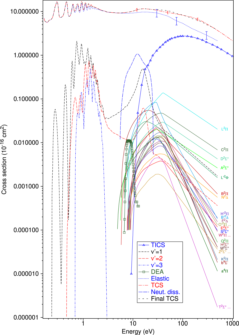
Brunger et al. [36] reported ICSs for 28 excited electronic states of NO, but only over the limited incident electron energy range 15–50 eV. Cartwright et al. [37] extended a subset of 9 of those cross sections, to their various threshold energies and out to 500 eV, in order to study the excited-state densities and band emissions of NO under auroral conditions. Here we extend the remaining 19 excited electronic-state ICSs to their respective threshold energies [38] and out to 500 eV, with all of these electronic-state ICSs being plotted in Fig. 1. Note that Xu et al. [39] reported some BE-scaling [8] theoretical results for the , and electronic states, and found good agreement with the ICSs of Brunger et al. [36] for the - and - states. For the -state, however, a discrepancy was noted although that may reflect on the applicability of using the BE-scaling approach for an electronic state with such a small optical oscillator strength [40]. For vibrational excitation we essentially adopt Figure 1 from Campbell et al. [41], which was constructed from the low-energy results of Josić et al. [42] and Jelisavcic et al. [43] and the higher-energy results of Mojarrabi et al. [44]. All these ICSs, for the = 0–1, 0–2 and 0–3 vibrational quanta, are plotted in Fig. 1. The present DEA cross sections were taken directly from Table 6 of Itikawa [27], being originally sourced from the work of Rapp and Briglia [45] (see Fig. 1). Similarly, the present TICS was taken directly from Table 5 of Itikawa [27], with the origin of the cross sections in this case being from Lindsay et al. [46] (again see Fig. 1). In the case of the elastic scattering, our initial data set is constructed below 3.38 eV by subtracting the present vibrational ICSs of Fig. 1 from the TCS measurement of Alle et al. [47]. Above 3.38 eV we use the recommended data from Table 2 of Itikawa [27]. The present elastic ICSs are also plotted in our Fig. 1. The TCSs of our initial cross section compilation were formed as follows. Below an incident electron energy of 2.6 eV we used the values of Alle et al. [47], as digitised from their Figure 1, while for above 5 eV we employed the values from Table 1 in Itikawa [27]. Between 2.6 eV and 5 eV we undertook an interpolation that ensured that the TCSs of Alle et al. [47] merged smoothly with those recommended by Itikawa [27]. The resultant TCS from this process is shown pictorially in Fig. 1. Finally, there remains the neutral dissociation cross section. There are no known measurements or calculations for the ND ICS in scattering, so our approach for estimating it was as follows. The sum of the individual ICSs, for all open scattering channels at some , should be consistent with the TCS, at least to within the uncertainties on the TCS. In this case, we found that when we summed all our ICSs there was a quite narrow energy region ( 5 – 20 eV) where it underestimated the TCS (to well outside the error on our TCS). We therefore assigned that residual cross section strength to be the ICS for ND, with our derived result again being plotted in Fig. 1.
Fig. 1 therefore summarises all the ICSs and the TCS that constitute our initial cross section compilation for input into our multi-term Boltzmann equation solver [18, 19], in order to determine transport coefficients that can be compared to corresponding independent results from electron-swarm experiments. The present error estimates on those ICSs and the TCS largely reflect those given in the original papers, from which our initial data base was derived. Typically, this would be on the elastic ICS, on the vibrational excitation ICS, on the TICS, in the range of – for the various electronic-state ICS, on the DEA ICS and on the ND ICS that we have derived. The independent TCS data set would have an error of , a little more than cited in the relevant papers as we have included a small additional uncertainty due to the so-called “forward angle scattering effect” [48] that was previously not allowed for. It is important to remember that, when using this initial cross section compilation in conjunction with a multi-term Boltzmann equation solver, the errors on the ICSs will in principle necessarily lead to a band of allowed solutions for the transport coefficients that are to be simulated.
Another observation we should make in respect to Fig. 1 is that it is clear that the TCS we determine from adding up all our various ICSs (denoted by - - - in black and called “Final TCS”) is entirely consistent with the TCS we derived from the independent measurements available to us (denoted by — - — in red). While this is a necessary condition for a cross section compilation to be plausibly physical, as we saw in our work on THF [18] and THFA [19] it by no means a priori guarantees that the simulated transport coefficients will reproduce the available swarm data. Finally, it is also relevant to note here that all the ICSs in the present compilation are rotationally averaged, which is a direct result of the energy resolution of current-day electron spectrometers not being narrow enough to resolve the various rotational lines [26].
3 Multi-term Boltzmann equation analysis of our initial set
To assess the quality of our initial set of electron-NO cross sections, we apply a well-benchmarked multi-term solution of Boltzmann’s equation [32, 49, 50] in order to calculate swarm transport coefficients for comparison to measured values in the literature. Chronologically, electron-NO swarm measurements include drift velocities and transverse characteristic energies by Skinker et al. [51] and Bailey et al. [52], transverse characteristic energies by Townsend [53], drift velocities and attachment coefficients by Parkes et al. [54], transverse characteristic energies and ionisation coefficients by Lakshminarasimha et al. [55], transverse and longitudinal characteristic energies by Mechlińska-Drewko et al. [56], and, most recently, drift velocities and longitudinal diffusion coefficients by Takeuchi et al. [33] (for both pure NO and admixtures of NO in Ar).
When performing a Boltzmann equation swarm analysis, it is essential to precisely interpret what is being measured in each swarm experiment under consideration [34, 57]. In this regard, many of the earlier electron-NO measurements are inadequate as they are obtained using a “magnetic deflection” experiment [58] that measures a drift velocity that is distinct from the bulk (centre-of-mass) drift velocity measured in pulsed-Townsend experiments [57] and provided by our Boltzmann solver. Ultimately, we choose to calculate comparisons to the drift velocities and longitudinal diffusion coefficients of Takeuchi et al. [33], the ionisation coefficients of Lakshminarasimha et al. [55], the attachment coefficients of Parkes et al. [54], the transverse characteristic energies of Lakshminarasimha et al. [55] and Mechlińska-Drewko et al. [56], and the longitudinal characteristic energies of Mechlińska-Drewko et al. [56] and Takeuchi et al. [33] (calculated using their drift and diffusion measurements). We purposefully leave out the 421 K measurements of Parkes et al. [54], due to an observed pressure dependence in their measured attachment coefficients that they attribute to electron detachment from product ions at this temperature. We also neglect the pure NO diffusion measurements of Takeuchi et al. [33] below 11 Td, due to the pressure dependence arising from three-body attachment in this low regime [59, 54]. While their associated drift velocity measurements also show a pressure dependence, it is to a far lesser extent and Takeuchi et al. [33] are able to consistently estimate pressure-independent values by extrapolation to zero pressure [33]. In almost all cases considered, we interpret swarm measurements as pertaining to the centre of mass of the swarm (i.e. bulk transport coefficients). The only exception we make is for the double-shutter drift tube experiment of Takeuchi et al. [33], which measures an “arrival time spectra” drift velocity, , that is distinct from the bulk drift velocity when nonconservative effects are present [34]. Fortunately, we can approximate this quantity in terms of our simulated bulk transport coefficients with [35]:
| (1) |
where is the bulk drift velocity, is the effective first Townsend ionisation coefficient, and is the bulk longitudinal diffusion coefficient.
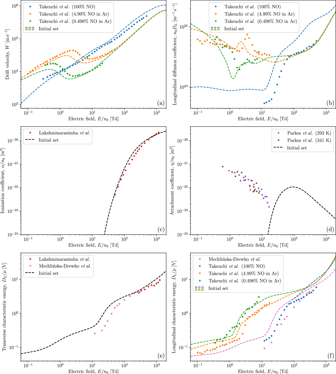
To perform the transport calculations, we require an appropriate quasielastic (elastic+rotation) momentum transfer cross section, which we obtain by multiplying the present elastic ICS (from Fig. 1) by the ratio of elastic MTCS to elastic ICS, each taken from the set of Itikawa [27]. When calculating the admixture transport coefficients, we use the argon cross section set present in the Biagi database [60, 61, 62]. The resulting simulated transport coefficients are plotted alongside the aforementioned experimental measurements in Figs. 2(a)–(f) for drift velocities, diffusion coefficients, ionisation coefficients, attachment coefficients, transverse characteristic energies, and longitudinal characteristic energies, respectively. Fig. 2(a) shows a qualitative agreement between our simulated drift velocities and the measurements of Takeuchi et al. [33]. In the case of pure NO, our initial cross section set results in drift velocities that are consistently too small below 2 Td and too large above 2 Td. In the admixture cases, the onset of negative differential conductivity (NDC) — the phenomenon of decreasing drift velocity with increasing — occurs earlier in our simulations than is shown by experiment. Fig. 2(b) indicates that our calculated longitudinal diffusion coefficients in pure NO are too large by roughly a factor of 2 on average. By comparison, the calculated admixture diffusion coefficients are much closer to the measurements and exhibit many of their qualitative features. We note that the two-term approximation is in error by up to 40% for the longitudinal diffusion coefficient measurements near 500 Td. It follows that a multi-term Boltzmann solver is also necessary here for the accurate calculation of characteristic energies. Fig. 2(c) shows ionisation coefficients calculated for our initial set that are generally larger than those measured by Lakshminarasimha et al. [55] (up to larger in some instances). Quantitatively, there is also room for improvement here. Fig. 2(d) shows the near absence of attachment in our simulations below , in stark contrast to the measurements of Parkes et al. [54]. This indicates the presence of a low-energy attachment process that is currently missing from our initial set. Fig. 2(e) shows a good quantitative agreement between our calculated transverse characteristic energies and those measured by Lakshminarasimha et al. [55]. However, the same cannot be said for the measurements of Mechlińska-Drewko et al. [56] which, while qualitatively similar, tend to be much smaller than what we calculate. Fig. 2(f) exhibits a disagreement between our calculated longitudinal characteristic energies and the pure NO measurements of Mechlińska-Drewko et al. [56] and Takeuchi et al. [33], both of which are consistently smaller than what we calculate. The agreement is much better for the mixture measurements of Takeuchi et al. [33], although the simulations are still larger than expected in the case of the 4.99% NO in Ar measurements below 3 Td.
4 Cross section refinement using data-driven swarm analysis
In the previous section, we have seen clear discrepancies between the transport coefficients calculated using our initial electron-NO cross section set and those determined experimentally by a number of authors. In this section, we apply machine learning in order to refine our initial set and hopefully improve its agreement with the measured swarm data plotted in Fig. 2.
4.1 Machine learning methodology
To obtain a solution to the inverse swarm problem, we utilise the artificial neural network of Stokes et al. [17, 18, 19]:
| (2) |
where are affine mappings defined by dense weight matrices and bias vectors , and is a nonlinear activation function [63] that is applied element-wise. The output vector, , contains each NO cross section of interest as a function of energy, , which is an element of the input vector, , alongside all of the swarm measurements plotted in Fig. 2. It should be noted that we apply suitable logarithmic transformations to ensure that all inputs and outputs of the network are dimensionless and lie within . We specify that each bias vector contains 256 parameters, with the exception of , the size of which must match the number of cross sections in . The weight matrices are all sized accordingly.
In order to train the neural network, Eq. (2), we require an appropriate set of example solutions to the inverse swarm problem. The choice of cross sections used for training is vital, in order for the network to provide a self-consistent and physically-plausible set of cross sections that are consistent within all the experimental error bars (including those on the TCS). We derive such cross sections from the LXCat project [23, 24, 25], as described in detail in Sec. 4.2 for each of the cross sections considered. Once suitable training cross sections are found, corresponding transport coefficients are determined using our multi-term Boltzmann solver [64, 49, 32] (here we use a four-term approximation). A small amount of random noise is also multiplied by each transport coefficient to roughly imitate random experimental error. The logarithm of this noise factor is sampled from a normal distribution with a mean of 0 and standard deviation of 0.03 for the drift velocities, 0.05 for the diffusion coefficients, and 0.1 for the ionisation coefficients, attachment coefficients and characteristic energies considered.
We implement and train the neural network, Eq. (2), using the Flux.jl machine learning framework [65]. The network is initialised such that its biases are zero and its weights are uniform random numbers, as described by Glorot and Bengio [66]. Training is performed using the AdaBelief optimiser [67] with Nesterov momentum [68, 69], step size , exponential decay rates and , and small parameter . At each iteration, the optimiser is provided with a different batch of 4096 training examples, where each batch consists of 32 training cross sections each evaluated at 128 random energies of the form where is sampled from a continuous uniform distribution. For each batch, the optimiser adjusts the neural network weights and biases with the aim of further minimising the mean absolute error in solving the inverse swarm problem for that batch. Training is continued for 150,000 iterations, providing an equal number of potential solutions to the inverse swarm problem. The quality of each of these solutions is subsequently assessed by calculating their corresponding transport coefficients and comparing these to the swarm data plotted in Fig. 2. The set that agrees best with the swarm measurements is presented below as our “refined” set.
4.2 Refined cross section set
Using our initial cross section set as a base, we apply the neural network, Eq. (2), to determine a selection of plausible NO cross sections underlying the the swarm measurements shown in Fig. 2. In particular, we determine cross sections for quasielastic (elastic+rotation) momentum transfer, neutral dissociation, and dissociative electron attachment.
For dissociative electron attachment, we keep the cross section from the initial set and determine an additional DEA cross section using physically-plausible training data of the form:
| (3) |
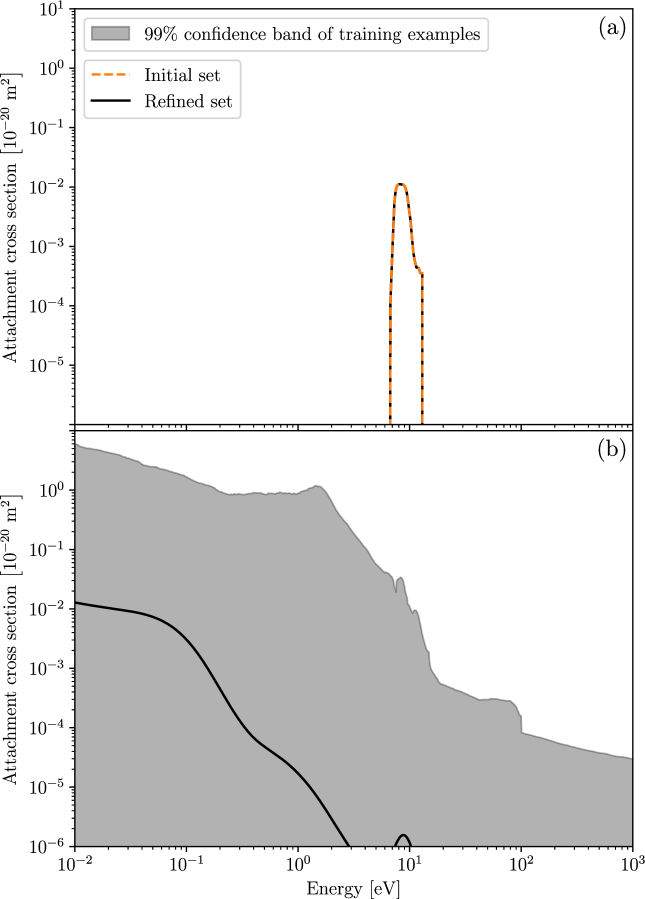
where is a mixing ratio sampled from a continuous uniform distribution, and and are a random pair of attachment cross sections from the LXCat project [23, 24, 25]. Beyond the implicit constraints due to the TCS (discussed below) and the physical constraints inherent to the LXCat cross sections, we otherwise leave the DEA training cross sections completely unconstrained. The resulting confidence band of training examples is plotted in Fig. 3(b), alongside the refined fit provided by the neural network. Fig. 3(a), on the other hand, simply shows that the DEA cross section from the initial set has remained unchanged in the refined set. As indicated by the attachment coefficient discrepancy shown in Fig. 2(d), the additional DEA cross section refined in Fig. 3(b) is largest at low energies. Below 0.1 eV, the refined DEA is roughly constant at , a magnitude comparable to the peak of the other, higher-energy, DEA process kept from the initial set. From 0.1 eV to 3 eV, the refined DEA cross section decays roughly according to a power law before vanishing. The refinement increases only very slightly in the vicinity of the other DEA process, near 9 eV, indicating that it is likely adequate as is.
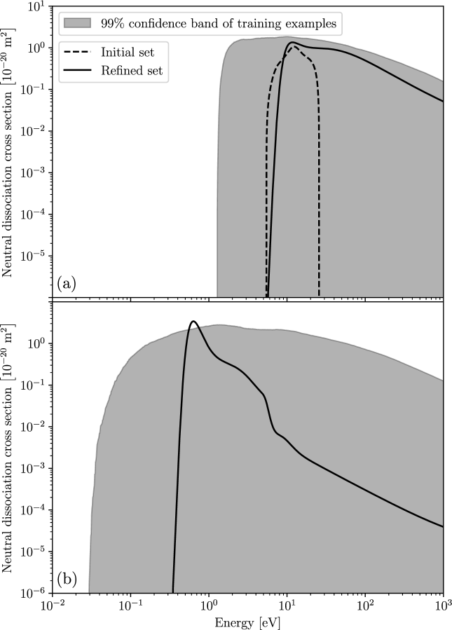
For neutral dissociation, we found that fitting a single unconstrained ND cross section resulted in a refinement with a threshold energy much lower than that for the ND proposed in the initial set (). It was only after attempting a fit with two unconstrained ND processes that a refined cross section of similar threshold energy arose. The training data used for these two processes took the form:
| (4) |
where and are a random pair of excitation cross sections from the LXCat project [23, 24, 25], and are their respective threshold energies, and is a uniformly sampled mixing ratio. We additionally use rejection sampling to enforce that the threshold energies of the two ND processes are at least apart. The resulting ND training example confidence bands are shown in Fig. 4. Fig. 4(a) indicates that the refined higher-threshold ND process has a threshold energy that is almost identical to its counterpart in the initial set (at versus ). While this refinement increases slowly from threshold compared to its counterpart, it ultimately reaches a slightly larger peak magnitude ( versus ) at a slightly lower energy (11.7 eV versus 12.3 eV). Beyond this turning point, the refinement decays monotonically, transitioning to power-law above 50 eV before falling to by 1000 eV. This is in stark contrast to the initial ND cross section, which lacks a high-energy tail due to its origin as a residual ICS from the TCS. Fig. 4(b) shows that the refined lower-threshold ND process has a threshold energy of . This refined cross section increases rapidly from threshold, reaching a peak magnitude of at 0.63 eV. The subsequent decay here is also monotonic, albeit somewhat more erratic, reaching a minimum of by 1000 eV.
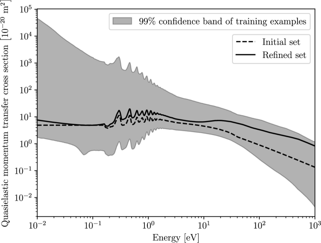
For the quasielastic momentum transfer cross section, we take a slightly different approach by using the neural network to determine a suitable energy-dependent scaling of the elastic ICS, which upon application would yield the refined quasielastic MTCS. The form of the scaling factors that are used for training is:
| (5) |
where is the quasielastic MTCS used for training, is the present elastic ICS, is the present quasielastic MTCS (i.e. from the initial set), and are random elastic cross sections formed from elastic cross sections on the LXCat project [23, 24, 25] that are combined using Eq. (3), and is a deterministic energy-dependent mixing ratio, used to constrain the quasielastic MTCS training data to lie in the vicinity of the experimental measurements of Mojarrabi et al. [44]:
| (6) |
Further, to ensure each quasielastic MTCS decays at high energies, we used rejection sampling to ensure that . The resulting quasielastic MTCS confidence band can be observed in Fig. 5, alongside the refined fit provided by the neural network, and the initial quasielastic MTCS for comparison. We see that the refined quasielastic MTCS is almost always larger than that from our initial set, with the difference becoming greater at higher energies. The greatest difference occurs at , where the tail of the refined quasielastic MTCS is almost an order of magnitude larger than that for the initial set.
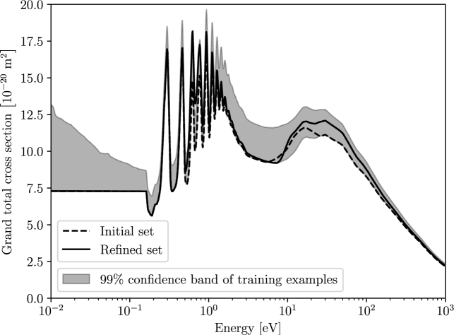
When sampling ND and DEA cross sections for training, we further employ rejection sampling to only keep cross section sets for training that lie within of the grand TCS of our initial set (while also accounting for the uncertainty in the elastic ICS of ). The resulting confidence band in the grand TCS, due to the training examples, is plotted in Fig. 6, alongside our initial and refined grand TCSs. The refined TCS is roughly the same as the initial TCS up until 10 eV, beyond which the refinement exceeds that we initially proposed. The greatest difference arises at 26 eV, with an increase in magnitude of 89%.
5 Multi-term Boltzmann equation analysis of our refined set
5.1 Consistency with swarm measurements
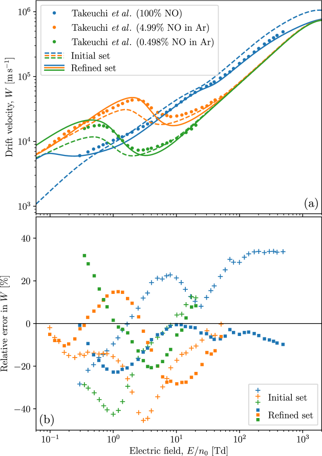
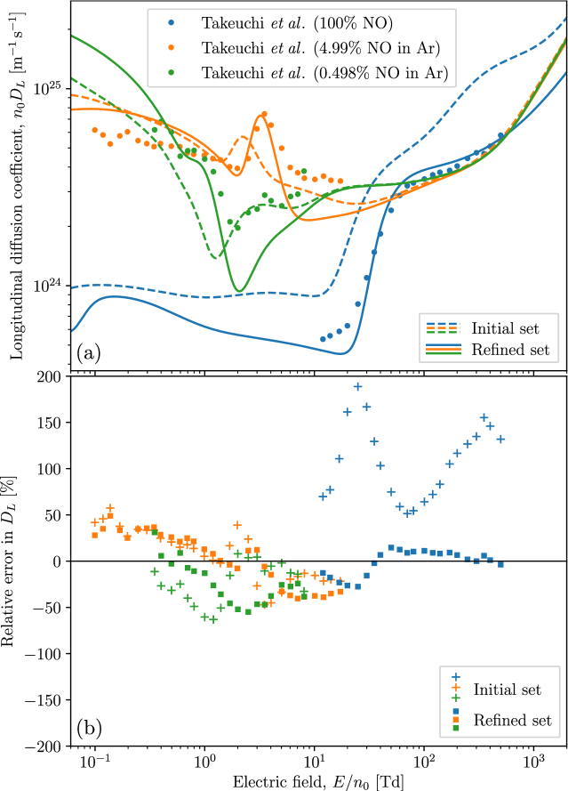
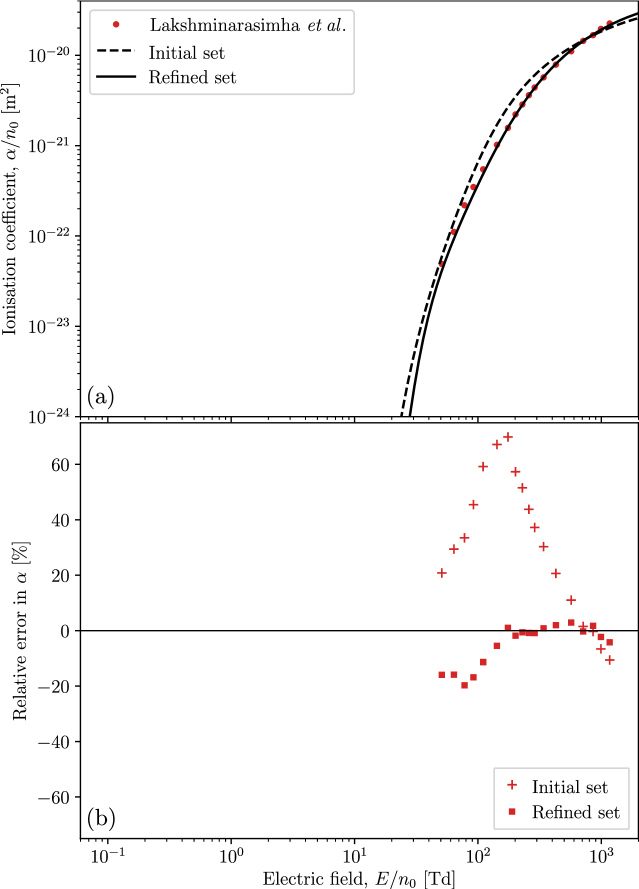
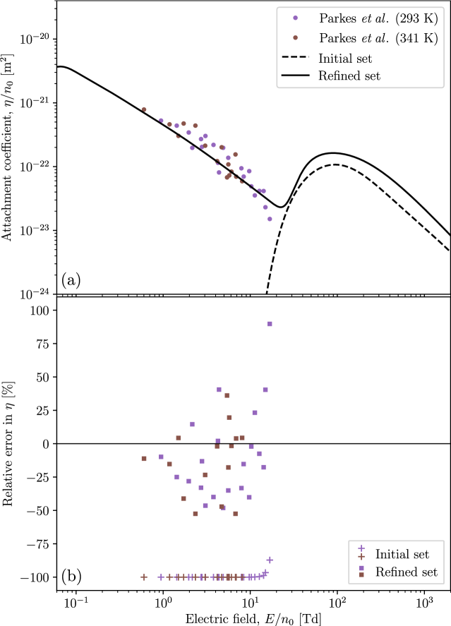
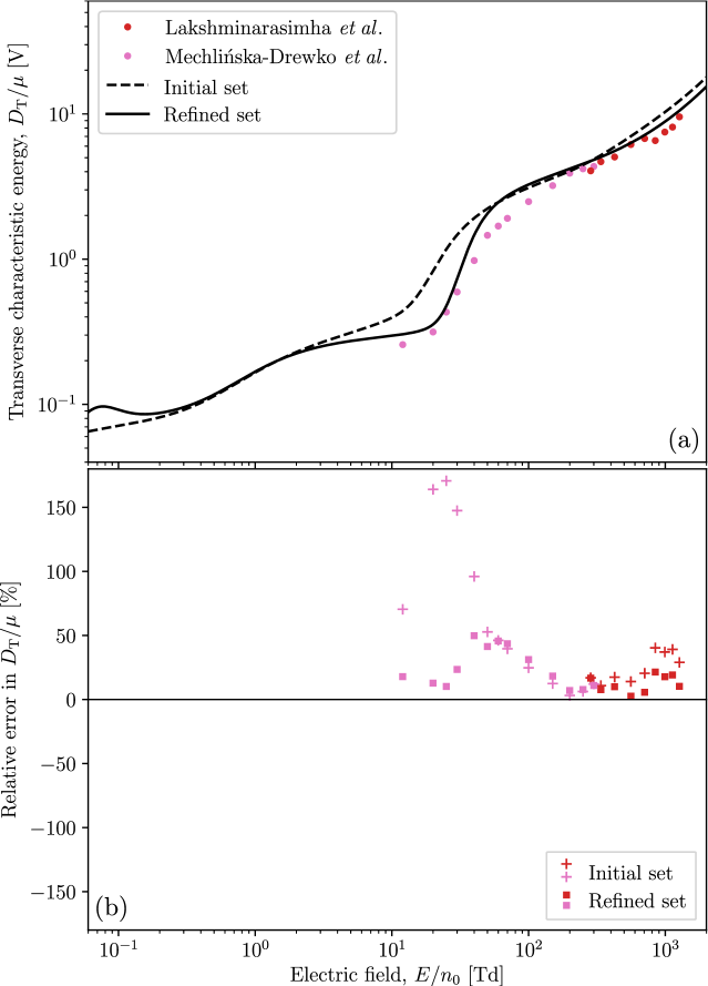
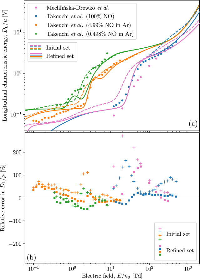
Using our refined set of electron-NO cross sections, we plot revised simulated transport coefficients in Figs. 7(a)–12(a) for comparison to the swarm measurements used to perform the refinement, as well as to the transport coefficients calculated previously using our initial set. These transport coefficients are accompanied by corresponding percentage difference (error) plots in Figs. 7(b)–12(b). Here, positive percentage differences indicate that our simulated transport coefficients exceed their experimentally-measured counterparts. Fig. 7 shows that our refined set has brought the simulated drift velocities much closer to the experimental measurements of Takeuchi et al. [33]. This agreement is particularly good for the pure NO measurements above 3 Td, with the discrepancies at lower possibly attributable to the drift velocities in this regime being estimated from pressure-dependent measurements [33]. Fig. 8 shows a large improvement after refinement for the pure NO diffusion measurements of Takeuchi et al. [33]. However, the outcome is somewhat more mixed in the case of diffusion measurements in the NO-Ar mixtures, with the refined set improving the agreement with some of the admixture measurements of Takeuchi et al. [33], while worsening it with others. Fig. 9 shows a significantly improved agreement between the ionisation coefficients of the refined set and the measurements of Lakshminarasimha et al. [55]. As this agreement was achieved without requiring adjustments to the initial TICS, this lends further credence to the overall self-consistency of the refinements that were made. Fig. 10 indicates that the attachment coefficient after refinement is non-zero below 20 Td, and in line with the measurements of Parkes et al. [54]. The accuracy here is now generally within , which is of the order of the uncertainty in the experimental measurements. Fig. 11 shows a transverse characteristic energy after refinement that agrees much better with the measurements of Mechlińska-Drewko et al. [56] and Lakshminarasimha et al. [55], while Fig. 12 shows similar improvements for the simulated longitudinal characteristic energy as compared to the measurements of Mechlińska-Drewko et al. [56] and Takeuchi et al. [33]. In this case, where the neural network was provided with both conflicting sets of pure NO measurements, the refined fit is seen here to be more consistent with the measurements of Takeuchi et al. [33] over those of Mechlińska-Drewko et al. [56].
5.2 Transport calculations for pure NO
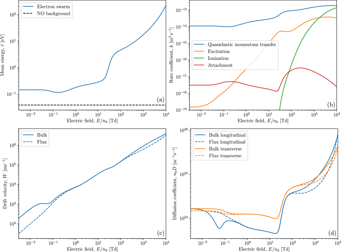
In Fig. 13, we apply our multi-term Boltzmann solver to our refined cross section set, in order to determine a variety of transport coefficients for electrons in NO at over a large range of reduced electric fields, , varying from to . We find that at least an eight-term approximation is necessary for all the considered NO transport coefficients to be accurate to within 1%. Fig. 13(a) shows a plot of mean electron energy alongside that for the background NO. In the low-field regime, the mean electron energy is , which is substantially higher than the thermal background of , a consequence of the attachment heating resulting from the refined DEA cross section in Fig. 3(b). As is increased, the onset of the vibrational excitation channels contributes to a net cooling of the electrons, causing the mean electron energy to reach a minimum of at . Beyond that point, increasing further causes the mean electron energy to increase monotonically due to heating by the field, with its ascent occasionally slowing due to the onset of additional excitation channels () and attachment and ionisation processes (). Fig. 13(b) shows the rate coefficients for quasielastic momentum transfer, summed discrete excitation, ionisation and attachment. The quasielastic momentum transfer rate coefficient is highly correlated with the mean electron energy, although this correlation tapers off near with a decrease with increasing . Summed excitation and ionisation rate coefficients both increase as expected with increasing . The summed attachment coefficient also behaves as expected, with the low-energy and high-energy attachment cross sections resulting in separate maxima at and , respectively. Fig. 13(c) shows the bulk (centre-of-mass) and flux drift velocities of the swarm, which are expected to differ when nonconservative processes are acting. For example, in the low-field regime, the preferential attachment of lower-energy electrons towards the back of the swarm results in a forward shift in the centre of mass, yielding a bulk drift velocity that is larger compared to its flux counterpart. Here, the bulk drift velocity also exhibits NDC between and . At intermediate fields, between and , net nonconservative effects are sufficiently small such that the bulk and flux drift velocities coincide. Above , the bulk drift velocity again exceeds the flux, this time due to ionisation preferentially creating electrons at the front of the swarm. Fig. 13(d) shows the bulk and flux diffusion coefficients in directions both longitudinal and transverse to the field. At very low , when the electron energy distribution function (EEDF) is nearly Maxwellian, the preferential attachment of low-energy electrons removes electrons from the centre of the swarm over those from the edges, causing an effective increase in the bulk diffusion coefficients compared to their flux counterparts. This remains the case transversely as increases due to the symmetry of the swarm in the transverse direction. Longitudinally, however, the additional power input by the field causes faster, higher energy, electrons to congregate at the front of the swarm, thus introducing an asymmetry in the longitudinal direction. The subsequent attachment of lower-energy electrons at the back of the swarm causes the bulk longitudinal diffusion coefficient to drop below its flux counterpart from , onward. As with the drift velocities, for intermediate between roughly 1 Td and 100 Td, nonconservative effects are minimal and the bulk and flux diffusion coefficients coincide. At higher , above 100 Td, there is a significant increase in bulk diffusion compared to flux in both the transverse and longitudinal directions, which we attribute to the preferential production of electrons due to ionisation at the front and sides of the swarm.
6 Conclusion
We have formed a comprehensive and self-consistent set of electron-NO cross sections, by constructing an initial set from the literature and then refining it using a multi-term Boltzmann equation analysis of the available swarm transport data. This refinement was performed automatically and objectively using a neural network model, Eq. (2), that was trained on cross sections derived from the LXCat project [23, 24, 25], to ensure that the refinements made were physically plausible. In summary, by using our initial set as a base, we obtained from the swarm data a quasielastic MTCS, a DEA cross section and a ND cross section. Compared to our initial set, we confirmed that our resulting refined cross section database was more consistent with the swarm data from which it was derived. Lastly, we used our refined set to calculate a variety of transport coefficients for electrons in NO across a large range of reduced electric fields. Notably, this revealed significant heating of the swarm above the thermal background due to our refined low-energy attachment process.
The machine learning methodology we have employed in this work has previously [18] been shown to produce cross section sets that are comparable to those refined using conventional swarm analysis, i.e. through manual iterative refinement by an expert. We thus believe that our refined set of electron-NO cross sections is of a similarly high quality. That said, we do acknowledge there is still some room for improvement in the present fit and it is thus fortunate that this machine learning approach makes it straightforward to revisit NO as new swarm data, cross section constraints, or LXCat training data becomes available. On this note, we highlight that there are presently no swarm measurements available for the effective first Townsend ionisation coefficient. We believe performing such measurements would be a worthwhile future endeavour, as they would allow one to quantify the attachment coefficient in the electropositive regime (above ) and thus allow for the possibility of refining the DEA cross section above .
Given the ill-posed nature of the inverse swarm problem, we also acknowledge that our refined set carries with it some uncertainty. In this sense, an artificial neural network of the form of Eq. (2) is not ideal as it does not provide uncertainty quantification. In the future, we may address this by using an appropriate alternative machine learning model [70, 71, 72, 73, 74, 75]. We also plan to apply our data-driven swarm analysis to determine complete and self-consistent cross section sets for other molecules of biological interest, including water [76].
Data Availability Statement
The data that supports the findings of this study are available within the article.
References
- [1] Kong M G, Kroesen G, Morfill G, Nosenko T, Shimizu T, Van Dijk J and Zimmermann J L 2009 New Journal of Physics 11 115012 ISSN 13672630 URL https://doi.org/10.1088/1367-2630/11/11/115012
- [2] Samukawa S, Hori M, Rauf S, Tachibana K, Bruggeman P, Kroesen G, Whitehead J C, Murphy A B, Gutsol A F, Starikovskaia S, Kortshagen U, Boeuf J P, Sommerer T J, Kushner M J, Czarnetzki U and Mason N 2012 Journal of Physics D: Applied Physics 45 253001 ISSN 0022-3727 URL https://doi.org/10.1088/0022-3727/45/25/253001
- [3] Bruggeman P J, Kushner M J, Locke B R, Gardeniers J G, Graham W G, Graves D B, Hofman-Caris R C, Maric D, Reid J P, Ceriani E, Fernandez Rivas D, Foster J E, Garrick S C, Gorbanev Y, Hamaguchi S, Iza F, Jablonowski H, Klimova E, Kolb J, Krcma F, Lukes P, MacHala Z, Marinov I, Mariotti D, Mededovic Thagard S, Minakata D, Neyts E C, Pawlat J, Petrovic Z L, Pflieger R, Reuter S, Schram D C, Schröter S, Shiraiwa M, Tarabová B, Tsai P A, Verlet J R, Von Woedtke T, Wilson K R, Yasui K and Zvereva G 2016 Plasma Sources Science and Technology 25 053002 ISSN 13616595 URL https://doi.org/10.1088/0963-0252/25/5/053002
- [4] Adamovich I, Baalrud S D, Bogaerts A, Bruggeman P J, Cappelli M, Colombo V, Czarnetzki U, Ebert U, Eden J G, Favia P, Graves D B, Hamaguchi S, Hieftje G, Hori M, Kaganovich I D, Kortshagen U, Kushner M J, Mason N J, Mazouffre S, Thagard S M, Metelmann H R, Mizuno A, Moreau E, Murphy A B, Niemira B A, Oehrlein G S, Petrovic Z L, Pitchford L C, Pu Y K, Rauf S, Sakai O, Samukawa S, Starikovskaia S, Tennyson J, Terashima K, Turner M M, Van De Sanden M C and Vardelle A 2017 Journal of Physics D: Applied Physics 50 323001 ISSN 13616463 URL https://doi.org/10.1088/1361-6463/aa76f5
- [5] Shekhter A B, Serezhenkov V A, Rudenko T G, Pekshev A V and Vanin A F 2005 Nitric Oxide 12 210–219 ISSN 10898603 URL https://doi.org/10.1016/j.niox.2005.03.004
- [6] Kim S J and Chung T H 2016 Scientific Reports 6 20332 ISSN 2045-2322 URL https://doi.org/10.1038/srep20332
- [7] Li Y, Ho Kang M, Sup Uhm H, Joon Lee G, Ha Choi E and Han I 2017 Scientific Reports 7 45781 ISSN 2045-2322 URL https://doi.org/10.1038/srep45781
- [8] Tanaka H, Brunger M J, Campbell L, Kato H, Hoshino M and Rau A R 2016 Reviews of Modern Physics 88 025004 ISSN 15390756 URL https://doi.org/10.1103/RevModPhys.88.025004
- [9] Mayer H F 1921 Annalen der Physik 369 451–480 ISSN 00033804 URL https://doi.org/10.1002/andp.19213690503
- [10] Ramsauer C 1921 Annalen der Physik 369 513–540 ISSN 15213889 URL https://doi.org/10.1002/andp.19213690603
- [11] Townsend J and Bailey V 1922 The London, Edinburgh, and Dublin Philosophical Magazine and Journal of Science 43 593–600 ISSN 1941-5982 URL https://doi.org/10.1080/14786442208633916
- [12] Frost L S and Phelps A V 1962 Physical Review 127 1621–1633 ISSN 0031899X URL https://doi.org/10.1103/PhysRev.127.1621
- [13] Engelhardt A G and Phelps A V 1963 Physical Review 131 2115–2128 ISSN 0031899X URL https://doi.org/10.1103/PhysRev.131.2115
- [14] Engelhardt A G, Phelps A V and Risk C G 1964 Physical Review 135 A1566–A1574 ISSN 0031-899X URL https://doi.org/10.1103/PhysRev.135.A1566
- [15] Hake R D and Phelps A V 1967 Physical Review 158 70–84 ISSN 0031899X URL https://doi.org/10.1103/PhysRev.158.70
- [16] Phelps A V 1968 Reviews of Modern Physics 40 399–410 ISSN 00346861 URL https://doi.org/10.1103/RevModPhys.40.399
- [17] Stokes P W, Cocks D G, Brunger M J and White R D 2020 Plasma Sources Science and Technology 29 055009 ISSN 13616595 (Preprint 1912.05842) URL https://doi.org/10.1088/1361-6595/ab85b6
- [18] Stokes P W, Casey M J, Cocks D G, de Urquijo J, García G, Brunger M J and White R D 2020 Plasma Sources Science and Technology 29 ISSN 13616595 (Preprint 2007.02762) URL https://doi.org/10.1088/1361-6595/abb4f6
- [19] Stokes P W, Foster S P, Casey M J, Cocks D G, González-Magaña O, De Urquijo J, García G, Brunger M J and White R D 2021 Journal of Chemical Physics 154 084306 ISSN 10897690 URL https://doi.org/10.1063/5.0043759
- [20] De Urquijo J, Casey M J, Serkovic-Loli L N, Cocks D G, Boyle G J, Jones D B, Brunger M J and White R D 2019 Journal of Chemical Physics 151 054309 ISSN 00219606 URL https://doi.org/10.1063/1.5108619
- [21] Morgan W L 1991 IEEE Transactions on Plasma Science 19 250–255 ISSN 19399375 URL https://doi.org/10.1109/27.106821
- [22] Ceriotti M, Clementi C and Anatole von Lilienfeld O 2021 The Journal of Chemical Physics 154 160401 ISSN 0021-9606 URL https://doi.org/10.1063/5.0051418
- [23] Pancheshnyi S, Biagi S, Bordage M C, Hagelaar G J, Morgan W L, Phelps A V and Pitchford L C 2012 Chemical Physics 398 148–153 ISSN 03010104 URL https://doi.org/10.1016/j.chemphys.2011.04.020
- [24] Pitchford L C, Alves L L, Bartschat K, Biagi S F, Bordage M C, Bray I, Brion C E, Brunger M J, Campbell L, Chachereau A, Chaudhury B, Christophorou L G, Carbone E, Dyatko N A, Franck C M, Fursa D V, Gangwar R K, Guerra V, Haefliger P, Hagelaar G J, Hoesl A, Itikawa Y, Kochetov I V, McEachran R P, Morgan W L, Napartovich A P, Puech V, Rabie M, Sharma L, Srivastava R, Stauffer A D, Tennyson J, de Urquijo J, van Dijk J, Viehland L A, Zammit M C, Zatsarinny O and Pancheshnyi S 2017 Plasma Processes and Polymers 14 1600098 ISSN 16128869 URL https://doi.org/10.1002/ppap.201600098
- [25] Carbone E, Graef W, Hagelaar G, Boer D, Hopkins M M, Stephens J C, Yee B T, Pancheshnyi S, van Dijk J and Pitchford L 2021 Atoms 9 16 ISSN 2218-2004 URL https://doi.org/https://doi.org/10.3390/atoms9010016
- [26] Brunger M J and Buckman S J 2002 Physics Reports 357 215–458 ISSN 03701573 URL https://doi.org/10.1016/S0370-1573(01)00032-1
- [27] Itikawa Y 2016 Journal of Physical and Chemical Reference Data 45 033106 ISSN 0047-2689 URL https://doi.org/10.1063/1.4961372
- [28] Song M Y, Yoon J S, Cho H, Karwasz G P, Kokoouline V, Nakamura Y and Tennyson J 2019 Journal of Physical and Chemical Reference Data 48 043104 ISSN 0047-2689 URL https://doi.org/10.1063/1.5114722
- [29] Brunger M J 2017 International Reviews in Physical Chemistry 36 333–376 ISSN 1366591X URL https://doi.org/10.1080/0144235X.2017.1301030
- [30] Sanz A G, Fuss M C, Muñoz A, Blanco F, Limão-Vieira P, Brunger M J, Buckman S J and García G 2012 International Journal of Radiation Biology 88 71–76 ISSN 0955-3002 URL https://doi.org/10.3109/09553002.2011.624151
- [31] Brunger M J, Ratnavelu K, Buckman S J, Jones D B, Muñoz A, Blanco F and García G 2016 The European Physical Journal D 70 46 ISSN 1434-6060 URL https://doi.org/10.1140/epjd/e2016-60641-8
- [32] White R D, Cocks D, Boyle G, Casey M, Garland N, Konovalov D, Philippa B, Stokes P, De Urquijo J, González-Magaa O, McEachran R P, Buckman S J, Brunger M J, Garcia G, Dujko S and Petrovic Z L 2018 Plasma Sources Science and Technology 27 053001 ISSN 13616595 URL https://doi.org/10.1088/1361-6595/aabdd7
- [33] Takeuchi T and Nakamura Y 2001 IEEJ Transactions on Fundamentals and Materials 121 481–486 ISSN 0385-4205 URL https://doi.org/10.1541/ieejfms1990.121.5%5F481
- [34] Robson R E, White R D and Ness K F 2011 The Journal of Chemical Physics 134 064319 ISSN 0021-9606 URL https://doi.org/10.1063/1.3544210
- [35] Kondo K and Tagashira H 1990 Journal of Physics D: Applied Physics 23 1175–1183 ISSN 0022-3727 URL https://doi.org/10.1088/0022-3727/23/9/007
- [36] Brunger M J, Campbell L, Cartwright D C, Middleton A G, Mojarrabi B and Teubner P J O 2000 Journal of Physics B: Atomic, Molecular and Optical Physics 33 809–819 ISSN 0953-4075 URL https://doi.org/10.1088/0953-4075/33/4/315
- [37] Cartwright D C, Brunger M J, Campbell L, Mojarrabi B and Teubner P J O 2000 Journal of Geophysical Research: Space Physics 105 20857–20867 ISSN 01480227 URL https://doi.org/10.1029/1999JA000333
- [38] Campbell L, Teubner P J O, Brunger M J, Mojarrabi B and Cartwright D C 1997 Australian Journal of Physics 50 525 ISSN 0004-9506 URL https://doi.org/10.1071/P96060
- [39] Xu X, Xu L Q, Xiong T, Chen T, Liu Y W and Zhu L F 2018 The Journal of Chemical Physics 148 044311 ISSN 0021-9606 URL https://doi.org/10.1063/1.5019284
- [40] Kato H, Kawahara H, Hoshino M, Tanaka H and Brunger M 2007 Chemical Physics Letters 444 34–38 ISSN 00092614 URL https://doi.org/10.1016/j.cplett.2007.06.134
- [41] Campbell L, Brunger M J, Petrovic Z L, Jelisavcic M, Panajotovic R and Buckman S J 2004 Geophysical Research Letters 31 n/a–n/a ISSN 00948276 URL https://doi.org/10.1029/2003GL019151
- [42] Josić L, Wróblewski T, Petrović Z, Mechlińska-Drewko J and Karwasz G 2001 Chemical Physics Letters 350 318–324 ISSN 00092614 URL https://doi.org/10.1016/S0009-2614(01)01310-0
- [43] Jelisavcic M, Panajotovic R and Buckman S J 2003 Physical Review Letters 90 203201 ISSN 0031-9007 URL https://doi.org/10.1103/PhysRevLett.90.203201
- [44] Mojarrabi B, Gulley R J, Middleton A G, Cartwright D C, Teubner P J O, Buckman S J and Brunger M J 1995 Journal of Physics B: Atomic, Molecular and Optical Physics 28 487–504 ISSN 0953-4075 URL https://doi.org/10.1088/0953-4075/28/3/019
- [45] Rapp D and Briglia D D 1965 The Journal of Chemical Physics 43 1480–1489 ISSN 0021-9606 URL https://doi.org/10.1063/1.1696958
- [46] Lindsay B G, Mangan M A, Straub H C and Stebbings R F 2000 The Journal of Chemical Physics 112 9404–9410 ISSN 0021-9606 URL https://doi.org/10.1063/1.481559
- [47] Alle D T, Brennan M J and Buckman S J 1996 Journal of Physics B: Atomic, Molecular and Optical Physics 29 L277–L282 ISSN 0953-4075 URL https://doi.org/10.1088/0953-4075/29/7/006
- [48] Brunger M J, Buckman S J and Ratnavelu K 2017 Journal of Physical and Chemical Reference Data 46 023102 ISSN 0047-2689 URL https://doi.org/10.1063/1.4982827
- [49] Boyle G J, Tattersall W J, Cocks D G, McEachran R P and White R D 2017 Plasma Sources Science and Technology 26 024007 ISSN 13616595 (Preprint 1509.00867) URL https://doi.org/10.1088/1361-6595/aa51ef
- [50] White R D, Robson R E, Schmidt B and Morrison M A 2003 Journal of Physics D: Applied Physics 36 3125–3131 ISSN 00223727 URL https://doi.org/10.1088/0022-3727/36/24/006
- [51] Skinker M and White J 1923 The London, Edinburgh, and Dublin Philosophical Magazine and Journal of Science 46 630–637 ISSN 1941-5982 URL https://doi.org/10.1080/14786442308634289
- [52] Bailey V and Somerville J 1934 The London, Edinburgh, and Dublin Philosophical Magazine and Journal of Science 17 1169–1176 ISSN 1941-5982 URL https://doi.org/10.1080/14786443409462470
- [53] Townsend J S 1948 Motion of Slow Electrons in Gases (London: Hutchinson)
- [54] Parkes D A and Sugden T M 1972 Journal of the Chemical Society, Faraday Transactions 2 68 600 ISSN 0300-9238 URL https://doi.org/10.1039/F29726800600
- [55] Lakshminarasimha C S and Lucas J 1977 Journal of Physics D: Applied Physics 10 313–321 ISSN 0022-3727 URL https://doi.org/10.1088/0022-3727/10/3/011
- [56] Mechlinska-Drewko J, Roznerski W, Petrovic Z L and Karwasz G P 1999 Journal of Physics D: Applied Physics 32 2746–2749 ISSN 0022-3727 URL https://doi.org/10.1088/0022-3727/32/21/306
- [57] Casey M J, Stokes P W, Cocks D G, Bošnjaković D, Simonović I, Brunger M J, Dujko S, Petrović Z L, Robson R E and White R D 2021 Plasma Sources Science and Technology 30 ISSN 13616595
- [58] Townsend J S E and Tizard H T 1913 Proceedings of the Royal Society of London. Series A, Containing Papers of a Mathematical and Physical Character 88 336–347 ISSN 0950-1207 URL https://royalsocietypublishing.org/doi/10.1098/rspa.1913.0034
- [59] Bradbury N E 1934 The Journal of Chemical Physics 2 827–834 ISSN 0021-9606 URL https://doi.org/10.1063/1.1749403
- [60] Biagi database URL www.lxcat.net/Biagi
- [61] Biagi S MAGBOLTZ
- [62] LXCat URL www.lxcat.net
- [63] Misra D 2019 (Preprint 1908.08681) URL http://arxiv.org/abs/1908.08681
- [64] White R D, Robson R E, Dujko S, Nicoletopoulos P and Li B 2009 Journal of Physics D: Applied Physics 42 194001 ISSN 00223727 URL https://doi.org/10.1088/0022-3727/42/19/194001
- [65] Innes M 2018 Journal of Open Source Software 3 602 ISSN 2475-9066 URL https://doi.org/10.21105/joss.00602
- [66] Glorot X and Bengio Y 2010 Understanding the difficulty of training deep feedforward neural networks Journal of Machine Learning Research (Proceedings of Machine Learning Research vol 9) ed Teh Y W and Titterington M (Chia Laguna Resort, Sardinia, Italy: PMLR) pp 249–256 ISSN 15324435 URL http://proceedings.mlr.press/v9/glorot10a.html
- [67] Zhuang J, Tang T, Ding Y, Tatikonda S C, Dvornek N, Papademetris X and Duncan J 2020 Advances in Neural Information Processing Systems 33
- [68] Nesterov Y 1983 Soviet Mathematics Doklady 27 372–376
- [69] Dozat T 2016 Incorporating Nesterov Momentum into Adam Proceedings of 4th International Conference on Learning Representations, Workshop Track
- [70] Bishop C M 1994 Mixture density networks URL http://publications.aston.ac.uk/id/eprint/373/
- [71] Sohn K, Lee H and Yan X 2015 Learning Structured Output Representation using Deep Conditional Generative Models Advances in Neural Information Processing Systems 28 ed Cortes C, Lawrence N D, Lee D D, Sugiyama M and Garnett R (Curran Associates, Inc.) pp 3483–3491 URL http://papers.nips.cc/paper/5775-learning-structured-output-representation-using-deep-conditional-generative-models.pdf
- [72] Mirza M and Osindero S 2014 (Preprint 1411.1784) URL http://arxiv.org/abs/1411.1784
- [73] Dinh L, Krueger D and Bengio Y 2015 3rd International Conference on Learning Representations, ICLR 2015 - Workshop Track Proceedings (Preprint 1410.8516) URL https://arxiv.org/abs/1410.8516
- [74] Dinh L, Sohl-Dickstein J and Bengio S 2017 5th International Conference on Learning Representations, ICLR 2017 - Conference Track Proceedings (Preprint 1605.08803) URL https://arxiv.org/abs/1605.08803
- [75] Kingma D P and Dhariwal P 2018 Glow: Generative flow with invertible 1×1 convolutions Advances in Neural Information Processing Systems vol 2018-Decem ed Bengio S, Wallach H, Larochelle H, Grauman K, Cesa-Bianchi N and Garnett R (Curran Associates, Inc.) pp 10215–10224 (Preprint 1807.03039) URL http://papers.nips.cc/paper/8224-glow-generative-flow-with-invertible-1x1-convolutions.pdf
- [76] White R D, Brunger M J, Garland N A, Robson R E, Ness K F, Garcia G, De Urquijo J, Dujko S and Petrović Z L 2014 European Physical Journal D 68 125 ISSN 14346079 URL https://doi.org/10.1140/epjd/e2014-50085-7